1.6.3 Parallel processing
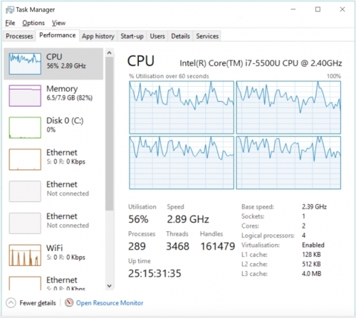
You have probably noticed if you have a relatively modern PC (anything from the last several years) that when you open Windows Task Manager (from the bottom of the list when you press CTRL-ALT-DEL) and you click the Performance tab and right click on the CPU graph and choose Change Graph to -> Logical Processors you have a number of processors (or cores) within your PC. These are actually “logical processors“ within your main processor but they function as though they were individual processors – and we’ll just refer to them as processors here for simplicity.
Now because we have multiple processors, we can run multiple tasks in parallel at the same time instead of one at a time. There are two ways that we can run tasks at the same time – multithreaded and multiprocessing. We’ll look at the differences in each in the following but it’s important to know that arcpy doesn’t support multithreading but it does support multiprocessing. In addition, there is a third form of parallelisation called distributed computing, which involves distributing the task over multiple computers, that we will also briefly talk about.
1.6.3.1 Multithreading
Multithreading is based on the notion of "threads" for a number of tasks that are executed within the same memory space. The advantage of this is that because the memory is shared between the threads they can share information. This results in a much lower memory overhead because information doesn’t need to be duplicated between threads. The basic logic is that a single thread starts off a task and then multiple threads are spawned to undertake sub-tasks. At the conclusion of those sub-tasks all of the results are joined back together again. Those threads might run across multiple processors or all on the same one depending on how the operating system (e.g. Windows) chooses to prioritize the resources of your computer. In the example of the PC above which has 4 processors, a single-threaded program would only run on one processor while a multi-threaded program would run across all of them (or as many as necessary).
1.6.3.2 Multiprocessing
Multiprocessing achieves broadly the same goal as multi-threading which is to split the workload across all of the available processors in a PC. The difference is that multiprocessing tasks cannot communicate directly with each other as they each receive their own allocation of memory. That means there is a performance penalty as information that the processes need must be stored in each one. In the case of Python a new copy of python.exe (referred to as an instance) is created for each process that you launch with multiprocessing. The tasks to run in multiprocessing are usually organized into a pool of workers which is given a list of the tasks to be completed. The multiprocessing library will assign each task to a worker (which is usually a processor on your PC) and then once a worker completes a task the next one from the list will be assigned to that worker. That process is repeated across all of the workers so that as each finishes a task a new one will be assigned to them until there are no more tasks left to complete.
You might have heard of the MapReduce framework which underpins the Hadoop parallel processing approach. The use of the term map might be confusing to us as GIS folks as it has nothing to do with our normal concept of maps for displaying geographical information. Instead in this instance map means to take a function (as in a programming function) and apply it once to every item in a list (e.g. our list of rasters from the earlier example).
The reduce part of the name is similar as we apply a function to a list and combine the results of our function into a single result (e.g. a list from 1 – 10,000 which is our number of Hi-ho Cherry-O games and we want the number of turns for each game).
The two elements map and reduce work harmoniously to solve our parallel problems. The map part takes our one large task (which we have broken down into a number of smaller tasks and put into a list) and applies whatever function we give it to the list (one item in the list at a time) on each processor (which is called a worker). Once we have a result, that result is collected by the reduce part from each of the workers and brought back to the calling function. There is a more technical explanation in the Python documentation [1].
Multiprocessing in Python
At around the same time that Esri introduced 64-bit processing, they also introduced multiprocessing to some of the tools within ArcGIS Desktop (mostly raster based tools in the first iteration) and also added multiprocessor support to the arcpy library.
Multiprocessing has been available in Python for some time and it’s a reasonably complicated concept so we will do our best to simplify it here. We’ll also provide a list of resources at the end of this section for you to continue exploring if you are interested. The multiprocessing package of Python is part of the standard library and has been available since around Python 2.6. The multiprocessing library is required if you want to implement multiprocessing and we import it into our code just like any other package using:
import multiprocessing
Using multiprocessing isn’t as simple as switching from 32-bit to 64-bit as we did above. It does require some careful thought about which processes we can run in parallel and which need to run sequentially. There are also issues about file sharing and file locking, performance penalties where sometimes multiprocessing is slower due to the time taken to setup and remove the multiprocessing pool, and some tasks that do not support multiprocessing. We’ll cover all of these issues in the following sections and then we’ll convert our simple, sequential raster processing example into a multiprocessing one to demonstrate all of these concepts.
1.6.3.3 Distributed processing
Distributed processing is a type of parallel processing that instead of (just) using each processor in a single machine will use all of the processors across multiple machines. Of course, this requires that you have multiple machines to run your code on but with the rise of cloud computing architectures from providers such as Amazon, Google, and Microsoft this is getting more widespread and more affordable. We won’t cover the specifics of how to implement distributed processing in this class but we have provided a few links if you want to explore the theory in more detail.
In a nutshell what we are doing with distributed processing is taking our idea of multiprocessing on a single machine and instead of using the 4 or however many processors we might have available, we're accessing a number of machines over the internet and utilizing the processors in all of them. Hadoop [2]is one method of achieving this and others include Amazon's Elastic Map Reduce [3], MongoDB [4]and Cassandra [5]. GEOG 865 [6] has cloud computing as its main topic, so if you are interested in this, you may want to check it out.