Print
The first FOSS product you'll use is a GUI-based program designed for desktop workstations. It's called QGIS (kyoo-jis), although you should know that sometimes in the past it was referred to as Quantum GIS. QGIS is somewhat similar in appearance and function to Esri's ArcMap, which you've likely used in previous courses.
In this tutorial, you'll install QGIS and make a basic vector map with it. You'll use some shapefiles of downtown Ottawa, Ontario, Canada that I originally downloaded from the OpenStreetMap database.
Download the Lesson 1 walkthrough data (It is a folder of shapefiles that you should extract into a folder such as c:\data).
- Visit the QGIS home page at www.qgis.org. Take a few minutes to explore this introductory page and any links that look interesting. This tells you a bit about who makes QGIS and what it can do.
- From the main QGIS page, click the Download Now Button.
The usability of this page has greatly improved in the past few years. Because FOSS can run on a variety of platforms and can be built directly from source code (as opposed to running an installer program), it's not uncommon with FOSS to see mind-boggling installation instructions with all manner of parenthetical warnings, stipulations, dependencies, and links to obscure download pages. This was previously the case with QGIS, but now the experience is much smoother. - You can now choose between the latest release of QGIS or the most recent long term release (LTR) version. The advantage of using the LTR version, (version 3.28 at the point of this writing) is that the examples in this course have been tested with this version and things on your screen will look very close to what is shown in the images you will see here. If you instead want to see all the features that QGIS has to offer right now and don't mind that things may look slightly different, feel free to go ahead and install the latest release. You can also install both version and switch between them.
To start the download, click on the large green button saying "Download QGIS ..." to download the most current release, or click the small link below it "Looking for the most stable version? ..." for the LTR version. Once you've downloaded it, run through the installation wizard and accept the default options:
QGIS can also run on Mac or Linux. You will see installation instructions for these platforms, and you are welcome to use them; however, only Windows instructions are given in these lesson materials. (I know this is paradoxical for a FOSS course, but teaching you to use Linux is outside the scope of these lessons.) If you get hung up, you may be expected to troubleshoot on your own or default to a Windows machine in order to complete the exercises. If all you know is Windows, I suggest you stick with Windows for this course.
The QGIS installation will place some other shortcuts and programs on your machine, such as GRASS GIS and OSGeo4W. This is fine. In fact, we will use some of these in later lessons. - Start QGIS. You can do this through the Windows Start Menu > All Programs > QGIS (Version name/number) > QGIS Desktop (Version number).
You will notice many toolbars available. In QGIS, the button you click to add data depends on the type of data source. For example, you click different buttons to add vector files, raster files, CSV files, web service layers, and layers from databases. - Drag the toolbars and windows around and clean up your display so that the layout looks something like the screenshot below (Figure 1.3). Don't worry about the order of the toolbars; just get them off the left-hand side if they show up there. You may have to explicitly add the "Manage Layers" toolbar to perfom the next step, as described below. Adding toolbars works the same as it does with ArcMap: just right-click any empty gray area around the toolbars and select the desired toolbar from the menu that appears. Alternatively, go View -> Toolbars in the main menu bar to toggle individual toolbars on and off.
- Click the button for adding vector data:

Once you've clicked the button to add vector data, click the ... button and browse to the roads.shp file from the lesson data folder. Even though a shapefile consists of multiple files, you just need to browse to the .shp when adding a shapefile in QGIS. Now click Add and then Close to close the window again.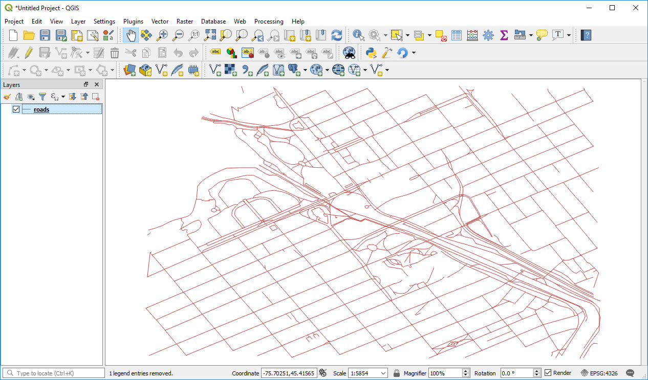 Figure 1.3
 - In the layer list, double-click the roads layer. You'll see a Symbology menu and a bunch of styling options where you can set the line color, the line width, a scale range for visibility, and labeling. Set the roads as a thin gray line.
Notice that in QGIS, you typically get a lot more symbol options if you highlight the deepest level of the symbol hierarchy, in this case, Simple line.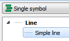
Note: During this walkthrough, I will provide general guidance about which settings to apply, and I will lead you to the correct neighborhood of dialog boxes to accomplish it; however, I will not provide point-and-click instructions for all actions. Although you may curse my name for this, I am doing it deliberately so that A) you can think about what you are doing and B) you can develop the habit of exploring new and unfamiliar software in a fearless manner. This is an essential skill if you are going to use FOSS.
That being said, it is not my intent to leave you frustrated and helpless. If something is not clear, please use the discussion forums to help each other out. I will regularly monitor the forums to make sure your question doesn't languish unanswered.
Next, we'll put some labels on the roads. - In the Layer Properties dialog box, use the Labels tab to label the roads layer with the roads' name attribute using a small gray font (this in the Text submenu). Set the label distance as 0.5 mm (this is in the Placement submenu of the Labels tab) so that the layer is not too close or too far away from the line. When working with streets, you might also want to check Merge connected lines to avoid duplicate labels (this is in the Rendering submenu). Finally, set Scale-based visibility (or Scale dependent visibility) preventing the labels from displaying when the map is zoomed out beyond 1:10000. When you are finished, you should have something like this.
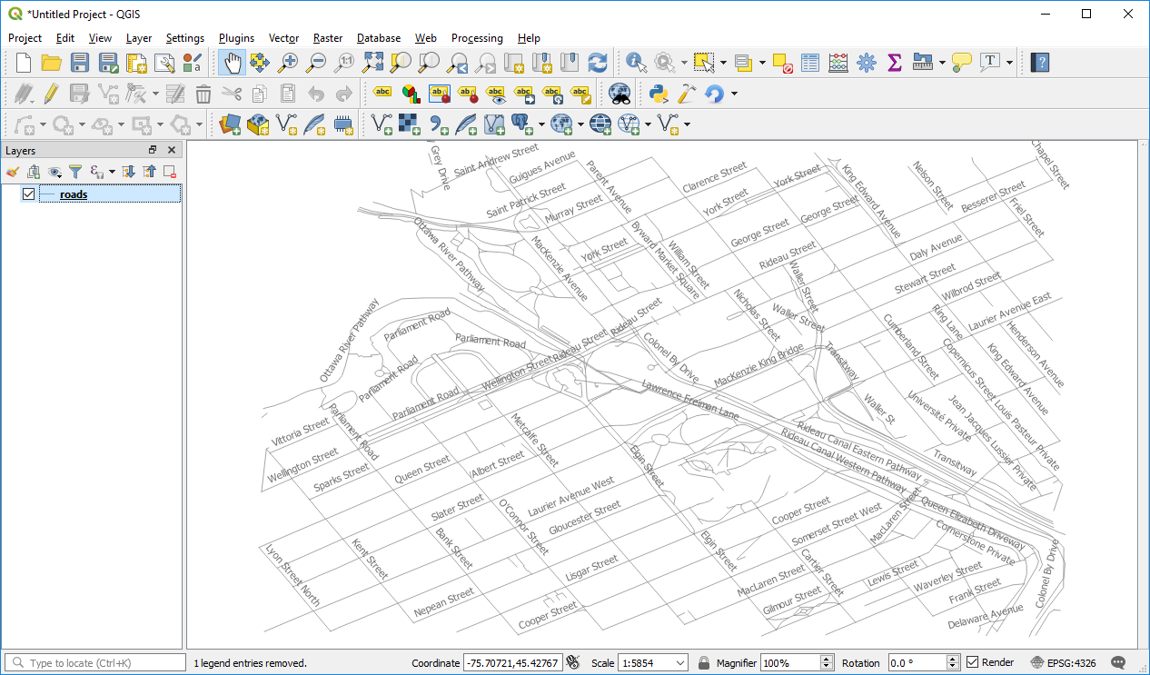 Figure 1.4
 - Add the dataset natural.shp and symbolize it as a light green fill with no outline. You will need to set the Stroke style to No pen in order to accomplish this.
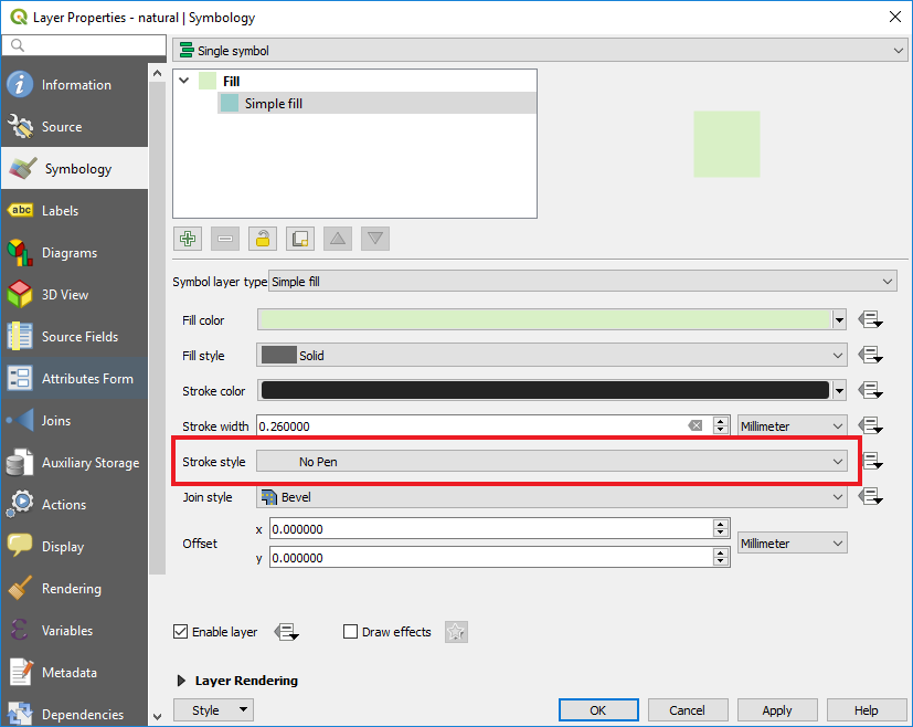 Figure 1.5
 - This is a good time to save your map. Click Project > Save As and save your map as Ottawa.qgz. It will be easiest if you save it in the same folder where your shapefiles live.
Note: You may be accustomed to using the .mxd format, and now is an opportune time to learn that .mxd is a proprietary format that is used by Esri software. QGIS uses an easily-readable XML format for storing projects (.qgs file) and the .qgz file is a zipped version of the .qgs file. You can also choose to store your project as an unzipped .qgs file and then open it in a text editor to inspect the XML code. However, .qgz is now the default file format for QGIS. - Add buildings.shp to the map, and experiment with a multilayer symbol to make the buildings “pop out.” Here's how I set this up:
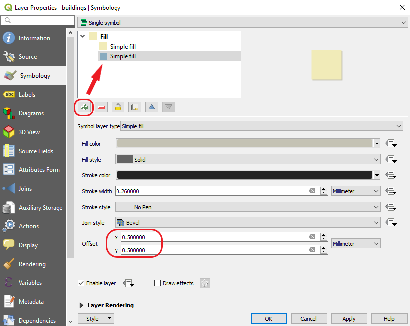 Figure 1.6
 - Add bus_stops.shp to the map, and symbolize it with an SVG marker that looks like a bus. In the Symbol layer type dropdown, select SVG marker like in the image below.
SVG stands for “scalable vector graphics.” It's a way of making marker symbols that don't get more pixelated as you expand their size. If you want a different color of marker, you can open the SVG in a graphics editing program such as the open source Inkscape, recolor and save a new version of the graphic, and then browse to it in QGIS.
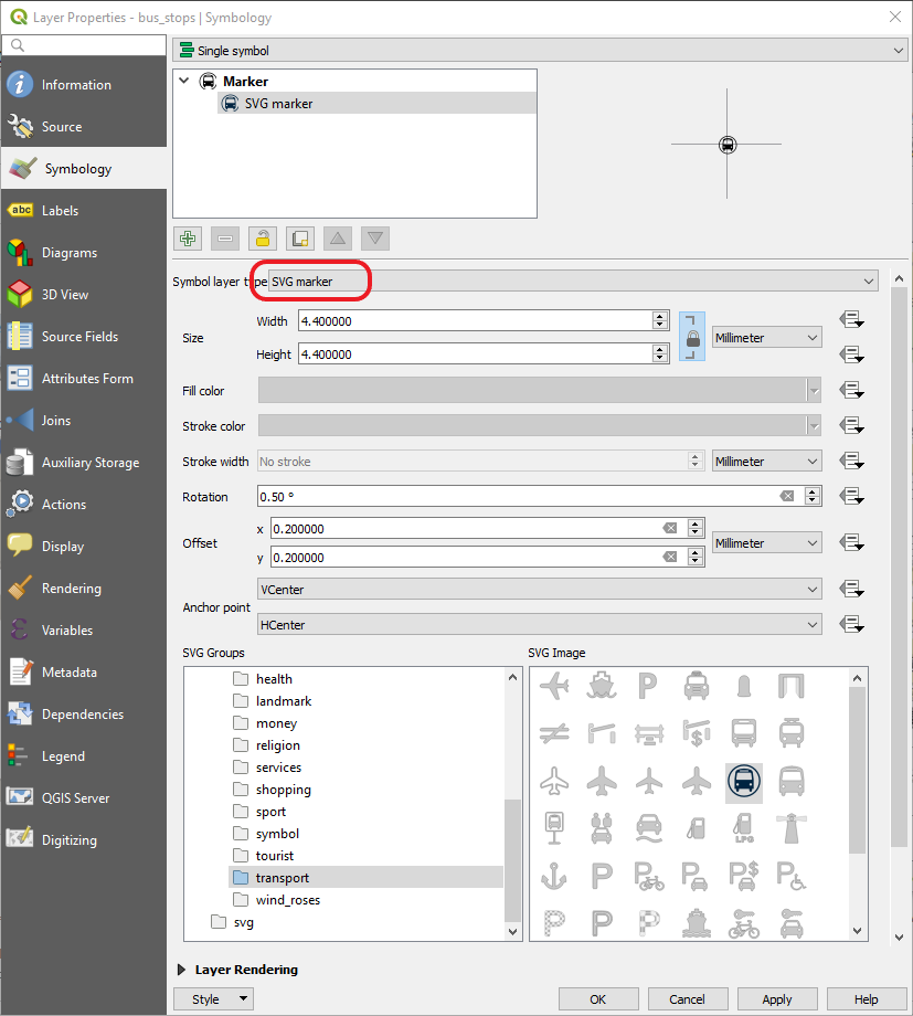 Figure 1.7
 - Set a scale range on the bus_stops layer so that it doesn't appear when zoomed out beyond 1:10000. You can do this in the Rendering tab.
This is also a good time to set a user-friendly display name for this and other layers. The display name appears in the layer list. You can change the display name in the Source tab.
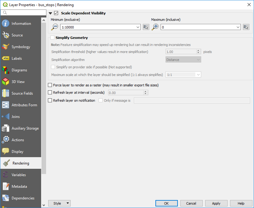 Figure 1.8
 - In the layer list, highlight the bus stops layer and click the Show Map Tips button. This button varies in appearance depending on the version of QGIS you're using, but in all cases it contains a little yellow speech bubble, like this
 . Map tips add some interactivity to the layer, a la Google Maps, so that when you hover over a stop for a short moment, the name of the corresponding bus line will be displayed. As we work with web maps during this course, we'll work with getting the same kind of interactivity for particular layers of interest.
In some versions of QGIS, this will show the bus stop ID number by default rather than the name. To remedy this, open the bus stops' Layer Properties again, go to the Display tab, and select the name field in the Display expression or Display name dropdown list.
Your map should now look something like the following: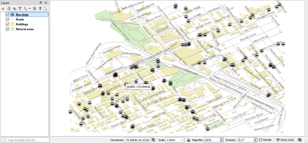 Figure 1.9
 - Save your map, then add some more shapefiles and experiment with symbolizing and labeling things in an aesthetically pleasing way.
- Post a screenshot of your beautiful QGIS map on the "Lesson 1 walkthrough result forum" on Canvas. Include some commentary about any features you found useful.