In this walkthrough, you'll get some practice serving some geographic data as a WMS using GeoServer. The exercise will progress from simple to complex in the following manner:
- Serving a single layer as a WMS using the default styling
- Applying a style to the WMS using an SLD
- Viewing the WMS in QGIS
The next walkthrough will go into more depth with SLDs and group layers.
As you complete these walkthroughs, think of some of your own data you'd like to serve as a WMS in fulfillment of the Lesson 4 assignment. You won't be required to use this WMS in your term project, but you can if you choose.
Serving a single layer as a WMS using the default styling
Let's start out by serving a single layer as a WMS. We'll stick with Philadelphia in this lesson so that we can eventually pull in some of the base layers that we clipped and projected previously. The first layer we'll work with is a polygon dataset of Philadelphia neighborhoods that I derived from a Zillow.com shapefile.
- Download Neighborhoods.zip and extract the contents into your Philadelphia data folder so that the files can be found at a path like c:\data\Philadelphia\Neighborhoods.shp. This data is already projected into EPSG:3857 and it doesn't need to be clipped for this exercise.
- Start GeoServer by running the startup.bat script from the bin subfolder.
- Start the GeoServer Web Admin Page by opening the URL localhost:8080/geoserver/web in your browser and log in with your administrator account (the username is probably "admin" with password "geoserver"). Refer to Lesson 2 if you need a refresher.
The first thing you will do is create a workspace and a store. A workspace is a place where you can organize datasets for a project. A store is an actual folder or database. A workspace can contain multiple stores. Our scenario is pretty simple because you'll have one workspace and one store; however, if your data were spread out among many folders or databases, you would need to create more stores. - In the left-hand menu, click Workspaces. You'll see some sample workspaces.
- Click Add New Workspace.
- In the Name field, type geog585.
- In the Namespace URI field type http://localhost:8080/geoserver/geog585 and then click Save. The Namespace URI doesn't have to be a real URL; it only needs to be a unique identifier. The GeoServer documentation suggests using a URL- like structure with the name of the workspace appended to it.
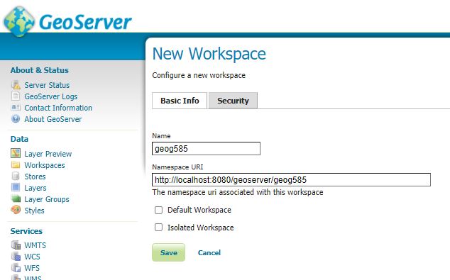 Figure 4.4 Configuring a new workspace in GeoServer
 - In the left-hand menu, click Stores and click Add New Store.
Examine the types of stores you can add. Notice that if you are going to use raster data with GeoServer, you need to add it as a separate store from your vector data. In this exercise, we'll just be working with the folder of vector shapefiles of Philadelphia that you've collected during this course. This should be located at a path similar to c:\data\Philadelphia. - Click Directory of spatial files (shapefiles).
- Complete the dialog box as in the graphic below, designating philadelphia as the name of the data source and browsing to your Philadelphia data folder where prompted to specify the directory of shapefiles.
When you are finished, click Save. Note that you can create this store even though there are raster files in it. If you wanted to use the rasters, though, you would have to specify a separate store in GeoServer.
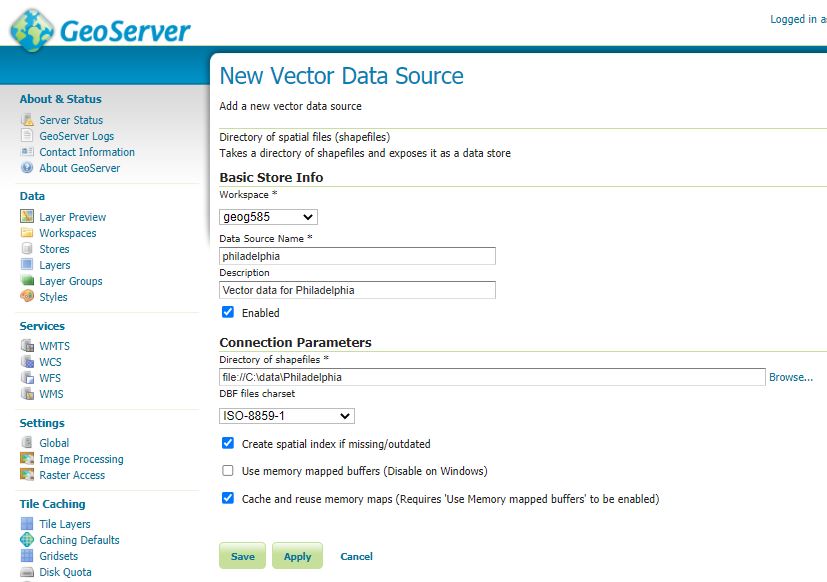 Figure 4.5 Defining a new vector data source in GeoServer
Now you will go one level further and specify the actual shapefile that you want to expose as a layer. - Click Layers > Add a New Layer. You'll be prompted to choose the store that will supply the layer.
- Choose to add the layer from geog585:philadelphia. You should see a list of layers from your Philadelphia folder.
- Find the Neighborhoods layer and click its Publish link.
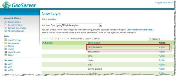 Figure 4.6 Adding the newly defined layer in GeoServer
 - At this point, you'll see a lot of options for publishing the layer. Leave the defaults near the top of the page, but scroll down until you come to the Coordinate Reference Systems section of the page and set it up as in the image below. Note that instead of manually filling in the bounding box coordinates, you just need to click the links Compute from data and Compute from native bounds in order to fill in the bounding boxes. Prior to doing this, you need to make sure you declare your SRS as EPSG:3857 (you must browse to this, not type it in) and that you set your SRS handling to Force declared. This allows you to serve data that is using the common web-based Mercator projection.
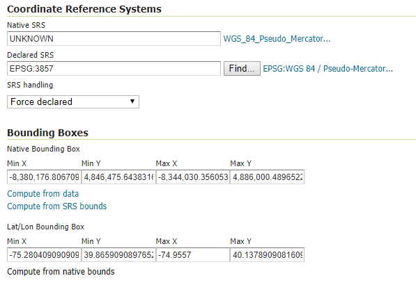 Figure 4.7 Setting the Coordinate Reference System (CRS) in GeoServer
Various programs have different ways of interpreting EPSG:3857, and some of them don't always match. I have found that if I do not set Force declared, my WMS is offset from other EPSG:3857 data by about 20 km when I try to display it all in QGIS. - Scroll down to the bottom of the page and click Save.
You should now see your layer appearing in the layer list. Let's take a look at it in a preview window. - In the left-hand menu, click Layer Preview. Then find your layer in the list.
- Choose to preview your layer as a WMS in the OpenLayers 3 example window.
You should see a basic map like this:
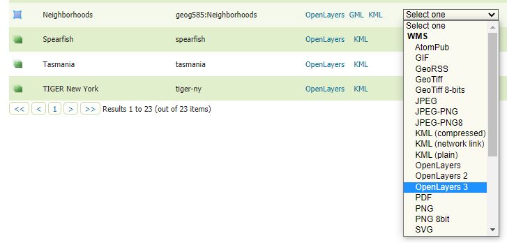 Figure 4.8 Setting up the preview of the new layer in GeoServerNotice the URL parameters above are the standard ones that you've learned about for WMS requests.
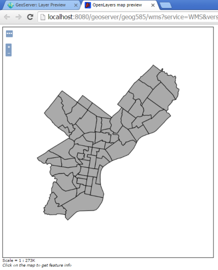 Figure 4.9 Output of the preview in GeoServer
Styling the WMS using SLDs
The above WMS indeed contains the Philadelphia neighborhoods, but there are no labels and we didn't get to choose the color scheme. In this part of the walkthrough, you'll use an SLD to apply a blue outline and labels with no fill. This will allow the neighborhoods WMS to act as a thematic layer that you can place on top of other base layers.
To work with SLDs in GeoServer, you first add the SLD under the Styles list. Then you can go back into the layer properties and apply the style. Decoupling the styles and the layers in this fashion allows you to reuse a particular style on multiple layers.
The first thing we'll do is prepare the SLD, starting with an existing sample and then modifying it to meet our needs.
- Open the SLD Cookbook to the Polygon with styled label example. This comes pretty close to what we want, so we're going to start with it.
- Click View and download the full "Polygon with styled label" SLD. You will see the XML of the SLD example.
- Use your browser's save option to save the page contents with a file extension of .sld. For example: polygonwithstyledlabel.sld
Do not copy and paste the XML out of the browser window, or you may fail to get the full XML headers and GeoServer won't like it. You must save the page as a .sld file. - Open the .sld file in a text editor like Notepad and take a close look at the PolygonSymbolizer and TextSymbolizer options. You should see something like this:
<?xml version="1.0" encoding="ISO-8859-1"?>
		<StyledLayerDescriptor version="1.0.0"
		    xsi:schemaLocation="http://www.opengis.net/sld StyledLayerDescriptor.xsd"
		    xmlns="http://www.opengis.net/sld"
		    xmlns:ogc="http://www.opengis.net/ogc"
		    xmlns:xlink="http://www.w3.org/1999/xlink"
		    xmlns:xsi="http://www.w3.org/2001/XMLSchema-instance">
		  <NamedLayer>
		    <Name>Polygon with styled label</Name>
		    <UserStyle>
		      <Title>SLD Cook Book: Polygon with styled label</Title>
		      <FeatureTypeStyle>
		        <Rule>
		          <PolygonSymbolizer>
		            <Fill>
		              <CssParameter name="fill">#40FF40</CssParameter>
		            </Fill>
		            <Stroke>
		              <CssParameter name="stroke">#FFFFFF</CssParameter>
		              <CssParameter name="stroke-width">2</CssParameter>
		            </Stroke>
		          </PolygonSymbolizer>
		          <TextSymbolizer>
		            <Label>
		              <ogc:PropertyName>name</ogc:PropertyName>
		            </Label>
		            <Font>
		              <CssParameter name="font-family">Arial</CssParameter>
		              <CssParameter name="font-size">11</CssParameter>
		              <CssParameter name="font-style">normal</CssParameter>
		              <CssParameter name="font-weight">bold</CssParameter>
		            </Font>
		            <LabelPlacement>
		              <PointPlacement>
		                <AnchorPoint>
		                  <AnchorPointX>0.5</AnchorPointX>
		                  <AnchorPointY>0.5</AnchorPointY>
		                </AnchorPoint>
		              </PointPlacement>
		            </LabelPlacement>
		            <Fill>
		              <CssParameter name="fill">#000000</CssParameter>
		            </Fill>
		            <VendorOption name="autoWrap">60</VendorOption>
		            <VendorOption name="maxDisplacement">150</VendorOption>
		          </TextSymbolizer>
		        </Rule>
		      </FeatureTypeStyle>
		    </UserStyle>
		  </NamedLayer>
		</StyledLayerDescriptor>
Notice the places where the stroke and fill colors are specified, as well as the text weight and font. Also notice the tags marked VendorOption, which are not part of all SLDs but are supported by GeoServer as a special means of finding suitable label locations (maxDisplacement) and forcing the labels to wrap after reaching a certain length (autoWrap). See this GeoServer documentation for details.
Let's edit the SLD to make a blue outline with a hollow fill, as well as blue labels. It is also critical that we change the name of the field that is supplying the label text (specified in the tag ogc:PropertyName). By default, in this example, the field is "name" but in our neighborhoods shapefile it is "NAME". The case sensitivity matters. - Replace your original SLD text with the following, either carefully editing line by line or completely copying and pasting the text below. Make sure you understand which lines changed and why.
<?xml version="1.0" encoding="ISO-8859-1"?>
		<StyledLayerDescriptor version="1.0.0"
		   xsi:schemaLocation="http://www.opengis.net/sld StyledLayerDescriptor.xsd"
		   xmlns="http://www.opengis.net/sld"
		   xmlns:ogc="http://www.opengis.net/ogc"
		   xmlns:xlink="http://www.w3.org/1999/xlink"
		   xmlns:xsi="http://www.w3.org/2001/XMLSchema-instance">
		  <NamedLayer>
		   <Name>Polygon with styled label</Name>
		   <UserStyle>
		    <Title>SLD Cook Book: Polygon with styled label</Title>
		    <FeatureTypeStyle>
		     <Rule>
		<PolygonSymbolizer>
		       <Stroke>
		        <CssParameter name="stroke">#133E73</CssParameter>
		        <CssParameter name="stroke-width">2</CssParameter>
		       </Stroke>
		      </PolygonSymbolizer>
		      <TextSymbolizer>
		       <Label>
		        <ogc:PropertyName>NAME</ogc:PropertyName>
		       </Label>
		       <Font>
		        <CssParameter name="font-family">Arial</CssParameter>
		        <CssParameter name="font-size">11</CssParameter>
		        <CssParameter name="font-style">normal</CssParameter>
		        <CssParameter name="font-weight">bold</CssParameter>
		       </Font>
		       <LabelPlacement>
		        <PointPlacement>
		         <AnchorPoint>
		          <AnchorPointX>0.5</AnchorPointX>
		          <AnchorPointY>0.5</AnchorPointY>
		         </AnchorPoint>
		        </PointPlacement>
		       </LabelPlacement>
		       <Fill>
		        <CssParameter name="fill">#133E73</CssParameter>
		       </Fill>
		       <VendorOption name="autoWrap">60</VendorOption>
		       <VendorOption name="maxDisplacement">150</VendorOption>
		      </TextSymbolizer>
		     </Rule>
		    </FeatureTypeStyle>
		   </UserStyle>
		  </NamedLayer>
		</StyledLayerDescriptor>
- Save this text file (making sure you keep the extension as .sld) and open the GeoServer Web Admin Page.
- In the GeoServer Web Admin Page, click the Styles link in the left-hand menu.
Notice there are some styles pre-loaded for you. You can also define your own, which we'll do. - Click Add a new style.
- Before giving the style a name and a workspace, scroll down below the code window and click the Choose File button under "Upload a style file".
- Browse to the .sld file you just created, then click the Upload link. You should see the code load into the window.
- Now name your SLD PolygonWithStyledLabel and place it in the geog585 workspace.
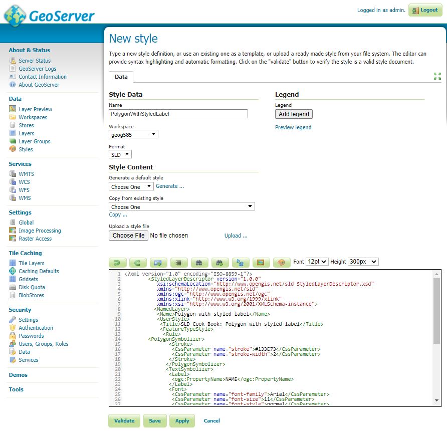 Figure 4.10 Defining / applying the new SLD in GeoServer
 - Scroll to the bottom of the page and click Save to create your style. Before doing this, you can click Validate to make sure your XML is acceptable to GeoServer.
You can come back to this page any time to make edits to your SLD. Any services using the SLD will be immediately updated.
Now let's apply this SLD to the neighborhoods layer. - In the left-hand menu, click Layers.
- Find your neighborhoods layer in the table and click the actual link that says Neighborhoods. This should take you to the Edit Layer page.
- Click the Publishing tab and scroll down to WMS Settings.
- In the Available Styles list, find your geog585:PolygonWithStyledLabel style and click the arrow button to move it over. Then set the Default style to PolygonWithStyledLabel.
Notice that a layer can advertise various styles, but you can choose which one gets applied by default. The alternate style in this case would be the basic gray polygon.
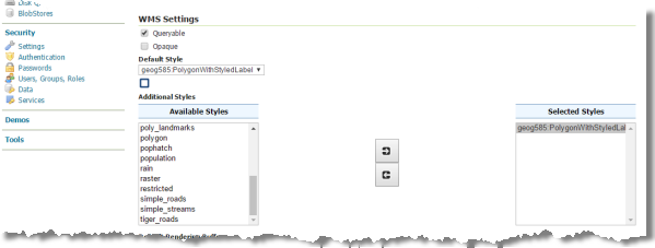 Figure 4.11
 - Click Save to preserve your changes.
- Use the Layer Preview link to preview your neighborhoods in the OpenLayers viewer as you did earlier in this walkthrough.
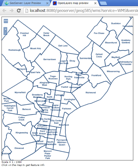 Figure 4.12 Preview of the data styled with our new SLD
This is still not perfect (notice the many labels overlapping features), but it is progress, and it has opened the door to editing the style through other XML options defined in the SLD and GeoServer documentation.
In general, labeling is a tricky subject with web maps. Labeling is computationally intensive and relies on complex rules that can slow down the map drawing. The labeling rules available with GeoServer and WMS are relatively simple compared to the logic used by a desktop program like QGIS or ArcMap. Because of these issues, web map authors sometimes rely on alternative mechanisms such as interactive popups or text that changes dynamically depending on where you point or click the mouse (or tap the display). Fetching this information on demand is faster than waiting for thousands of labels to be placed and eliminates the reliance on complex labeling algorithms.
Viewing the WMS in QGIS
There are lots of clients you can use to view a WMS. You already saw how your WMS could be previewed with OpenLayers. Now let's take a few minutes to see how QGIS works with WMS layers. This is important if you want to bring web services into your desktop maps as backgrounds or thematic layers.
- Launch QGIS, start a new project, and click the Add WMS/WMTS Layer button.

- In the Layers tab, click the New button. Here you will put the properties of your GeoServer workspace. All the layers in your workspace are exposed through the same root WMS URL.
- Enter the name as Geog585 Layers and the URL as http://localhost:8080/geoserver/geog585/wms as shown below. Notice that the geog585 in the URL is the name of the workspace you created in GeoServer.
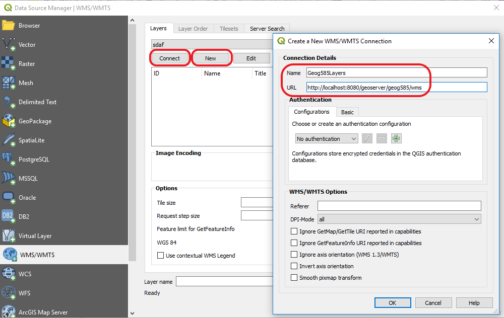 Figure 4.13 WMS connection dialog
 - Click OK and then click Connect.
- Select the Neighborhoods layer and click Change. A WMS by default can display itself in EPSG:4326 (WGS 84 geographic coordinates) or any other coordinate systems that the server administrator would like to support. Your WMS supports EPSG:3857 and that's what you'd like to request from the server here in your maps.
- Set the coordinate reference system to EPSG:3857 and click OK.
- Make sure your dialog box looks like the one below. Click Add to add the layer, and then click Close to close the dialog box.
You should see the layer added to the display like this:
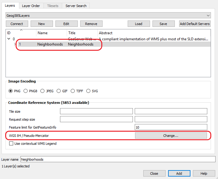 Figure 4.14 QGIS Add WMS layer dialogThis is a good time to use the OpenLayers plugin that you may already have installed in Lesson 3. At the end, I'll also explain how you can do the same thing without the OpenLayers plugin.
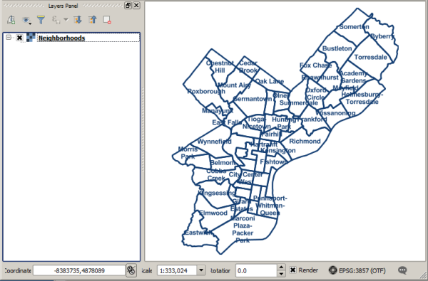 Figure 4.15 QGIS layer list example
First of all, if you did not install the OpenLayers plugin, please have a look at section "Processing spatial data with FOSS" again. Let's put a simple basemap beneath this to give it some geographic context. - In QGIS, click Web > OpenLayers plugin > OSM/Stamen > Stamen Watercolor/OSM.
- Rearrange your layers so that the OSM streets are on the bottom.
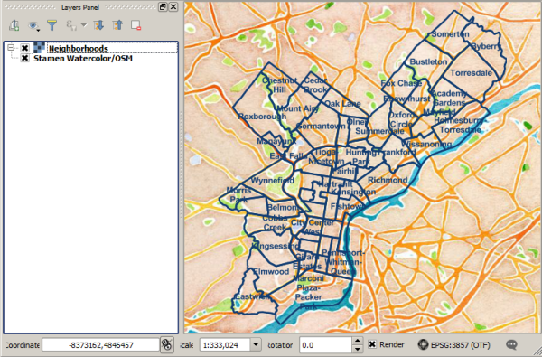 Figure 4.16 QGIS sample output showing our WMS layer and a styled OpenStreetMap layer
If you don't have the OpenLayers plugin installed, you can still add the Stamen Watercolor map. You do this by pointing QGIS at the basemap image tiles on the Stamen servers. First, make sure your Browser panel is open. If necessary, click View > Panels > Browser. In the list of layer types in the Browser panel, find the XYZ Tiles item, right-click it, and choose New Connection. Enter the Name as "Stamen watercolor" and enter the URL as http://c.tile.stamen.com/watercolor/{z}/{x}/{y}.jpg . This is the generic URL structure for the Stamen Watercolor tiled map images (more on this in Lesson 5), where x is the column, y is the row, and z is the zoom level of the tile to fetch at any given map extent. Click OK, and then drag and drop the resulting Stamen Watercolor layer down into your map layer list in the Layers panel. See this post for tips on adding all kinds of other basemap layers to QGIS 3 in the same fashion.
Congratulations! You have just made a (somewhat strange) "mashup" that brings in web services from two different servers. In future lessons, you'll learn how to do this in a more practical fashion in a web application.
QGIS not only displays WMS layers; it can also help you create SLDs. In the next walkthrough, you'll make some SLDs using QGIS and learn how to group WMS layers together using GeoServer.