Lesson 3: Storing and processing spatial data with FOSS
The links below provide an outline of the material for this lesson. Be sure to carefully read through the entire lesson before returning to Canvas to submit your assignments.
Note: You can print the entire lesson by clicking on the "Print" link above.
Overview
Underneath any web map are spatial datasets representing the entities to be placed on the map and their various attributes. In this lesson, you will learn about FOSS options for storing and processing spatial data. The broad scope of this course prohibits a full discussion of database theory and design; however, you will hopefully learn enough to select the appropriate type of data format for your project. Once you get your data in order, you'll be ready to launch GIS web services and assemble them into a web map.
Objectives
- List common open formats for spatial data and give appropriate uses for each.
- Recognize the advantages of various data storage architectures and formats.
- Process (clip and project) GIS data using QGIS and GDAL, and describe when it would be appropriate to use each.
- Experiment with a new GDAL function and use the documentation to learn how to invoke it.
Checklist
- Read the Lesson 3 materials on this page.
- Complete the two walkthroughs.
- Complete the Lesson 3 assignment.
- Complete the "First quiz" on Canvas. This covers material from Lessons 1 - 3.
Some common open formats for spatial data
This section of the lesson describes in greater detail some of the spatial data formats that have open specifications or are created by open source software. Note that these refer to files or databases that can stand alone on your hardware. We will cover open formats of web services streamed in from other computers in future lessons.
File-based data
File-based data includes shapefiles, KML files, GeoJSON, and many other types of text-based files. Each of the vector formats has some mechanism of storing the geometry (i.e., vertex coordinates) and attributes of each feature. Some of the formats, such as KML may also store styling information.
Below are some of the file-based data formats you're most likely to encounter.
Shapefiles
The Esri shapefile is one of the most common formats for exchanging vector data. It actually consists of several files with the same root name, but with different suffixes. At a minimum, you must include the .shp, .shx, and .dbf files. Other files may be included in addition to these three when extra spatial index or projection information is included with the file. This ArcGIS Resources article [1] gives a quick overview of the different files that can be included.
Because a shapefile requires multiple files, it is often expected that you will zip them all together in a single file when downloading, uploading, and emailing them.
If you want to make a shapefile from scratch, you can refer to the specification from Esri [2]. This is not for the novice programmer, and browsing this spec will hopefully increase your appreciation for those who donate their time and skills to coding FOSS GIS programs.
GeoPackages
The GeoPackage [3] is a relatively new format for storing and transferring vector features, tables, and rasterized tiles across a variety of devices, including laptops, mobile devices, and so forth. It was defined by the Open Geospatial Consortium (OGC), a group you will learn about in more detail in Lesson 4 that consists of industry representatives, academics, practitioners, and others with an interest in open geospatial data formats. The GeoPackage actually stores the data in a SQLite database, described below in more detail in the databases section. I list the GeoPackage here in the file-based formats section because some have advocated [4] for its adoption as a more modern alternative to the shapefile.
KML
KML gained widespread use as the simple spatial data format used to place geographic data on top of Google Earth. It is also supported in Google Maps and various non-Google products.
KML stands for Keyhole Markup Language, and was developed by Keyhole, Inc., before the company's acquisition by Google. KML became an Open Geospatial Consortium (OGC) standard data format in 2008, having been voluntarily submitted by Google.
KML is a form of XML, wherein data is maintained in a series of structured tags. At the time of this writing, the Wikipedia article for KML [5] contains a simple example of this XML structure. KML is unique and versatile in that it can contain styling information, and it can hold either vector or raster formats ("overlays", in KML-speak). The rasters themselves are not written in the KML, but are included with it in a zipped file called a KMZ. Large vector datasets are also commonly compressed into KMZs.
GeoJSON and TopoJSON
JavaScript Object Notation (JSON) is a structured means of arranging data in a hierarchical series of key-value pairs that a program can read. (It's not required for the program to be written in JavaScript.) JSON is less verbose than XML and ultimately results in less of a "payload," or data size, being transferred across the wire in web applications.
Following this pattern, GeoJSON is a form of JSON developed for representing vector features. The GeoJSON spec [6] gives some basic examples of how different entities such as point, lines, and polygons are structured.
You might choose to save GeoJSON features into a .js (JavaScript) file that can be referenced by your web map. Other times, you may encounter web services that return GeoJSON.
A variation on GeoJSON is TopoJSON [7], which stores each line segment as a single arc that can be referenced multiple times by different polygons. In other words, when two features share a border, the vertices are only stored once. This results in a more compact file, which can pay performance dividends when the data needs to be transferred from server to client.
Other text files
Many GIS programs can read vector data out of other types of text files, such as .gpx (popular format for GPS tracks) and various types of .csv (comma-separated value files often used with Microsoft Excel) that include longitude (X) and latitude (Y) columns. You can engineer your web map to parse and read these files, or you may want to use your scripting skills to get the data into another standard format before deploying it in your web map. This is where Python skills and helper libraries can be handy.
Various raster formats
Most raster formats are openly documented and do not require royalties or attribution. These include JPEG, PNG, TIFF, BMP, and others. The GIF format previously used a patented compression format, but those patents have expired.
Web service maps such as WMS return their results in raster formats, as do many tiled maps. A KML/KMZ file can also reference a series of rasters called overlays.
Spatially-enabled databases
When your datasets get large or complex, it makes sense to move them into a database. This often makes it easier to run advanced queries, set up relationships between datasets, and manage edits to the data. It can also improve performance, boost security, and introduce tools for performing spatial operations.
Below are described several popular approaches for putting spatial data into FOSS databases. Examples of proprietary equivalents include Microsoft SQL Server, Oracle Spatial, and the Esri ArcSDE middleware (packaged as an option with ArcGIS Enterprise) that can connect to various flavors of databases, including FOSS ones.
PostGIS
PostGIS is an extension that allows spatial data management and processing within PostgreSQL (often pronounced "Postgress" or "Postgress SQL"). PostgreSQL is perhaps the most fully featured FOSS relational database management system (RDBMS). If a traditional RDBMS with relational tables is your bread and butter, then PostgreSQL and PostGIS are a natural fit if you are moving to FOSS. The installation is relatively straightforward: in the latest PostgreSQL setup programs for Windows, you just check a box after installation indicating that you want to add PostGIS. An importer wizard allows you to load your shapefiles into PostGIS to get started. The rest of the administration can be done from the pgAdmin GUI program that is used to administer PostgreSQL.
Most FOSS GIS programs give you an interface for connecting to your PostGIS data. For example, in QGIS you might have noticed the button Add PostGIS Layers  . The elephant in the icon is a symbol related to PostgreSQL. GeoServer also supports layers from PostGIS.
This course, Geog 585, does not provide walkthroughs for PostGIS; however, there are a couple of excellent open courseware lessons in Geog 868: Spatial Databases [8] that describe how to install and work with PostGIS. I encourage you to make time to study these on your own (or take the instructor-led offering) if you feel that learning PostGIS will be helpful in your career.
You are welcome to use PostGIS in your term project if you feel comfortable with the other course material and want to take on an additional challenge. You can always fall back on file-based data if an excessive amount of troubleshooting is required.
SpatiaLite
SpatiaLite is an extension supporting spatial data in the SQLite database. As its name indicates, SQLite is a lightweight database engine that gives you a way to store and use data in a database paradigm without installing any RDBMS software on the client machine. This makes SQLite databases easy to copy around and allows them to run on many kinds of devices. If you are familiar with Esri products, a SpatiaLite database might be thought of as similar to a file geodatabase.
SpatiaLite is not as mature as PostGIS, but it is growing in popularity, and you will see a button in QGIS called Add SpatiaLite Layer  . If you feel it would be helpful in your career, you are welcome to use SpatiaLite in your term project. If you choose to do this, I ask you to first get the project working with file-based data. Then feel free to experiment with swapping out the data source to SpatiaLite.
You will encounter a SpatiaLite database in the Lesson 9 walkthrough when you use QGIS to import data from OpenStreetMap. In that scenario, you are dealing with a large amount of data with potentially many fields of complex attributes. SpatiaLite is a more self-contained and flexible choice than shapefiles, KML, etc., for this type of task.
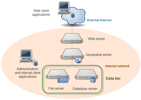
The Data Tier Of Your Web Mapping Architecture
In the previous lesson, you learned that system architectures for web mapping include a data tier. This could be as simple as several shapefiles sitting in a folder on your server machine, or it could be as complex as several enterprise-grade servers housing an ecosystem of standalone files and relational databases. Indeed, in our system architecture diagram, I have represented the data tier as containing a file server and a database server.
The data tier contains your datasets that will be included in the web map. Almost certainly, it will house the data for your thematic web map layers. It may also hold the data for your basemap layers, if you decide to create your own basemap and tile sets. Other times, you will pull in basemaps, and quite possibly some thematic layers, from other peoples' servers, relieving yourself of the burden of maintaining the data.
Some organizations are uneasy with the idea of taking the same database that they use for day-to-day editing and putting it on the web. There is justification for this uneasiness, for both security and performance reasons. If you are allowing web map users to modify items in the database, you want to avoid the possibility of your data being deleted, corrupted, or sabotaged. Also, you don't want web users' activities to tax the database so intensely that performance becomes slow for your own internal GIS users, and vice versa.
For these reasons, organizations will often create a copy or replica of their database and designate it solely for web use. If features in the web map are not designed to be edited by end users, this copy of the database is read-only. If, on the other hand, web users will be making edits to the database, it is periodically synchronized with the internal "production" database using automated scripts or web services. A quality assurance (QA) step can be inserted before synchronization if you would prefer for a GIS analyst to examine the web edits before committing them to the production database.
Where to put the data? On the server or its own machine?
You can generally increase web map performance by minimizing the number of "hops" between machines that your data has to take before it reaches the end user. If your data is file-based or is stored in a very simple database, you may just be able to store a copy of it directly on the machine that hosts your geospatial web services, thereby eliminating network traffic between the geospatial server and a data server. However, if you have a large amount of data, or a database with a large number of users, it may be best to keep the database on its own machine. Isolating the database onto its own hardware allows you to use more focused backup and security processes, as well as redundant storage mechanisms to mitigate data loss and corruption. It also helps prevent the database and the server competing for resources when either of these components is being accessed by many concurrent users.
If you choose to house your data on a machine separate from the server, you need to ensure that firewalls allow communication between the machines on all necessary ports. This may involve consulting your IT staff (bake them cookies, if necessary). You may also need to ensure that the system process running your web service is permitted to read the data from the other machine. Finally, you cannot use local paths such as C:\data\Japan to refer to the dataset; you must use the network name of the machine in a shared path; for example, \\dataserver\data\Japan.
Files vs. databases
When designing your data tier, you will need to decide whether to store your data in a series of simple files (such as shapefiles or KML) or in a database that incorporates spatial data support (such as PostGIS or SpatiaLite). A file-based data approach is simpler and easier to set up than a database if your datasets are not changing on a frequent basis and are of manageable size. File-based datasets can also be easier to transfer and share between users and machines.
Databases are more appropriate when you have a lot of data to store, the data is being edited frequently by different parties, you need to allow different tiers of security privileges, or you are maintaining relational tables to link datasets. Databases can also offer powerful native options for running SQL queries and calculating spatial relationships (such as intersections).
If you have a long-running GIS project housed in a database, and you just now decided to expose it on the web, you'll need to decide whether to keep the data in the database or extract copies of the data into file-based datasets.
Open data formats and proprietary formats
To review a key point from the previous section, in this course, we will be using open data formats, in other words, formats that are openly documented and have no legal restrictions or royalty requirements on their creation and use by any software package. You are likely familiar with many of these, such as shapefiles, KML files, JPEGs, and so forth. In contrast, proprietary data formats are created by a particular software vendor and are either undocumented or cannot legally be created from scratch or extended by any other developer. The Esri file geodatabase is an example of a well-known proprietary format. Although Esri has released an API for creating file geodatabases, the underlying format cannot be extended or reverse engineered.
Some of the most widely-used open data formats were actually designed by proprietary software vendors, who made the deliberate decision to release them as open formats. Two examples are the Esri shapefile and the Adobe PDF. Although opening a data format introduces the risk that FOSS alternatives will compete with the vendor's functionality, it increases the interoperability of the vendor's software, and, if uptake is widespread, augments the vendor's clout and credibility within the software community.
Processing spatial data with FOSS
Imagine you've identified some spatial data to use in your web map, but the data doesn't quite fit your purposes yet. It covers a broader region than your study area, and you want it to be in a different projection. Maybe you have a raster DEM that you need to convert into a hillshade, or perhaps you want to interpolate some raster surfaces that you can use in a time series animation. Indeed, a large portion of your datasets will probably need some kind of preprocessing before you incorporate them into your web map.
In these situations, you need to:
- identify the FOSS tools that can help you do the data processing;
- learn how to use the tools successfully;
- take notes on what you did so that you remember how to do it in the future!
If you're accustomed to a proprietary GIS software package that contains hundreds of tools and uniform documentation out of the box, it may seem frustrating to move to FOSS. Cobbling together a range of tools and collecting bits or pieces of documentation may seem like a waste of precious time. This is the tradeoff that you make when you use free software. Fortunately, the number of operations to learn is finite, and most of the time you'll probably be doing one of a dozen or fewer common actions, such as selecting data, projecting, clipping, and buffering. After you've learned how to do these once, you can go back and repeat the steps with any dataset, especially if you have taken good notes. Also, scripting these actions or running them in batch may require less overhead and processing time than you experience with proprietary software.
This is not a course about spatial data processing; however, this particular lesson attempts to give you some experience doing data processing with FOSS. You will learn a few resources for addressing data processing, and you'll get a feel for how to approach new tools.
Tools you will use in this course for data processing
In this course, you'll use QGIS and its associated plugins as a GUI tool for data processing. You will also learn how to use the GDAL and OGR command line utilities. These are explained in more detail below.
QGIS
QGIS offers a lot of the most common vector and raster processing tools out of the box. Additionally, developers in the QGIS user community have contributed plugins that can extend QGIS functionality.
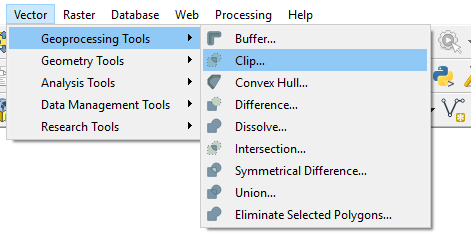
Open QGIS and explore the Vector menu to see some of the operations for processing vector data. You'll notice tools for merging, summarizing, intersecting, buffering, clipping, and more.
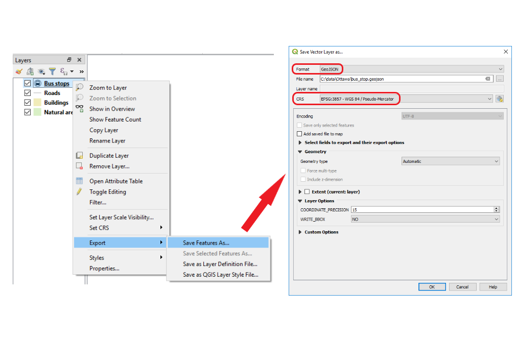
Some of the most powerful options are hidden in the Export context menu item when you right-click a vector layer. The Save Features As... dialog box allows you to convert data between different formats (for example, convert a shapefile to GeoJSON) and reproject the data to a new coordinate system.
Now, go back up to the top of the QGIS screen and click the Raster menu to see some of the options for processing rasters. Notice that you can warp, clip, contour, and interpolate to raster formats, along with various other operations.
In addition to these common vector and raster processing options, the Processing > Toolbox menu at the top of the QGIS screen gives you a dockable side window with access to many additional functions, some of them more obscure than others. This toolbox is akin to the full "ArcToolbox" that you see in Esri software. One difference is that it contains tools from multiple software packages, including GDAL, GRASS, and SAGA (a popular open source library for processing rasters). One of the more common "algorithms" (as they are called in QGIS) that I use in this toolbox is Create Grid, which can create square or hexagon lattices for cartographic "binning" or, in other words, aggregation to uniformly shaped regions in order to get a better visualization of a point pattern. Creating a lattice of hexagons is a task not easy to do by hand, and is well-suited to a pre-canned tool.
If you don't see what you're looking for in any of the above locations, someone may have developed a plugin for it. QGIS comes with a few of the more useful plugins already installed. Click Plugins > Manage And Install Plugins to see what they are. Here, you can disable some of these plugins if you don't like them getting in the way.
If you want to add more plugins, you can do it directly from this dialog box by clicking Not installed. Do this now, and examine the descriptions of some of the plugins you can add (the list may vary from what you see below).

You can even pick one and install it if you like. The OpenLayers plugin shown above is a handy way to see OpenStreetMap, Google Maps, etc. in QGIS. This plugin is still declared "experimental" in QGIS 3, so most likely you will only be able to see the plugin if you first click on the Settings tab and select the option to show experimental plugins. The plugin will add a new entry in the Web menu, from which you can pick different basemap options. Be aware that the quality and usability of the plugins may vary.
GDAL and OGR utilities
Many spatial data processing functions use well-known logic or documented algorithms. It would cause extra tedious work and possibly introduce errors and inconsistency if every FOSS developer had to code these same operations from scratch. Therefore, many FOSS programs take advantage of a single open source code library called GDAL (Geospatial Data Abstraction Library) to perform the most common functions.
GDAL is most commonly thought of as a raster processing library. But within GDAL is an important repository of vector processing functions called the OGR Simple Features Library. You will hear the terms GDAL and OGR many times as you work with FOSS, so get used to them. You can thank a man named Frank Warmerdam for initiating and maintaining these libraries over time. Although you may have never heard of him, you've probably done something to run his code at one point or another.
One way to use GDAL and OGR is by launching functions from QGIS or some other GUI-based program, like you would get from the menu options pictured above. Another way is to write code in Python, C#, or some other language that calls directly into these libraries. A third way, which lies in the middle in terms of complexity and flexibility, is to call into GDAL and OGR using command line utilities. These utilities were installed for you when you installed QGIS. You will get a feel for them in the lesson walkthrough.
Other tools
There are many other FOSS tools out there for wrangling spatial data; new ones appear all the time. Later in this course you'll be required to find one, test it out, review it, and share it with the class. Be an explorer, and if you find something that works for you, stick with it. You can certainly use any FOSS tool that works for you in order to complete the term project.
Walkthrough: Clipping and projecting vector data with QGIS and OGR
This walkthrough will first give you some experience using the GUI environment of QGIS to clip and project some vector data. Then, you'll learn how to do the same thing using the OGR command line utilities. The advantage of the command line utility is that you can easily run it in a loop to process an entire folder of data.
This project introduces some data for Philadelphia, Pennsylvania that we're going to use throughout the next few lessons. Most of these are simple basemap layers that I downloaded and extracted from OpenStreetMap; however, the city boundary is an official file from the City of Philadelphia that I downloaded from PASDA [10].
Download the Lesson 3 vector data [11]
Clipping and projecting data with QGIS
- Extract the dataset to a simple path such as C:\data\PhiladelphiaBaseLayers.
- Open the folder and explore it a bit. You'll see a bunch of shapefiles that you can add to QGIS and examine. Also, notice that I have created three folders in preparation for our exercise: clipFeature, clipped, and clippedAndProjected.
- These datasets use a geographic coordinate system and cover the large region of greater Philadelphia. Our processing task is to clip them to the Philadelphia city boundary, then project them into the modified Mercator coordinate system used by popular online web maps (like Google, Bing, Esri, and so forth).
- First, we'll clip and project a dataset using QGIS. This is an easy way to process a single dataset, especially if you're using a tool for the first time.
- Launch QGIS and add fuel.shp and clipFeature/city_limits.shp to the map.
- Click Vector > Geoprocessing Tools > Clip.
- Set the Input vector layer as fuel and the Clip layer as city_limits. Set the output shapefile to be saved in the subfolder as clipped/fuel.shp as shown below. You need to click the ... button, then choose Save to File... and select .SHP for the output format.
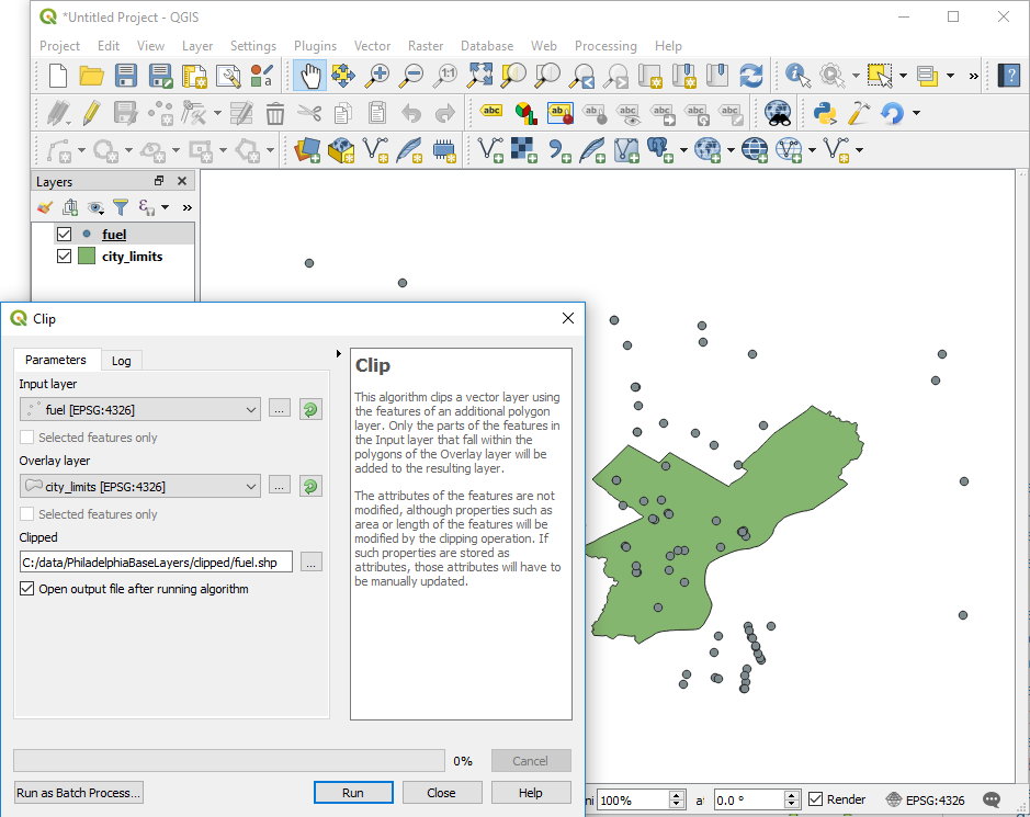 Figure 3.5 Clip tool GUI
 - Select the checkbox for adding the result to the canvas ("Open output file after running algorithm") so you can verify your work. Then click Run. The new layer should only contain features within the boundary of Philadelphia.
Now, let's project this dataset. In QGIS, you do this by saving out a new layer.
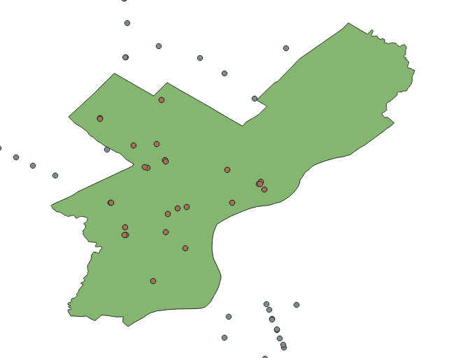 Figure 3.6 Clip tool results
 - In the table of contents, right-click the clipped fuel dataset (not the original one!) and click Export -> Save Features As.... Make sure that the Format box is set to ESRI Shapefile.
- Next to the File name box where you are prompted to put a path, click the ... button and set the path for the output dataset as clippedAndProjected/fuel.shp.
- Next to the CRS box, click the Select CRS button on the right. This is where you'll specify the output projection. The nice thing is that you can search.
- In the Filter box, type pseudo and select WGS 84 / Pseudo Mercator (EPSG: 3857) (not EPSG: 6871). Then click OK.
This projection has lots of names, and we'll cover more of its history in other lessons. For now, remember that you can recognize it using its EPSG code which should be 3857. (Most projections have EPSG codes to overcome naming conflicts and confusion).
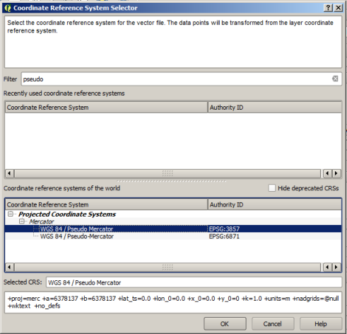 Figure 3.7 QGIS Coordinate reference system dialog
 - Click OK to save out the projected layer. A good way to verify it worked is to start a new map project and add it.
- Create a new map project in QGIS (there's no need to save the old one) and add the clippedAndProjected/fuel.shp file. The layout of the features should look something like what you see below. (I put an SVG marker symbol on this as in Lesson 1, just for fun.)
In QGIS, just like in ArcMap, the first layer you add to the map determines the projection. Notice how the EPSG code in the lower right corner is 3857, proving that my data was indeed projected. If you add any of our other layers to this map, make sure you add them after you add the fuel layer for this reason.
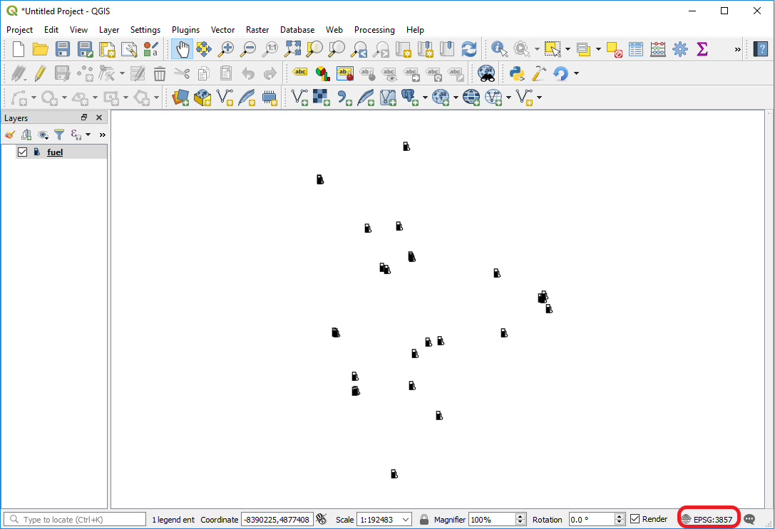 Figure 3.8 Sample QGIS layout showing updated map projection
Clipping and projecting data using the OGR command line utilities
That was easy enough, but it would be tedious, time-consuming, and possibly error prone if you had to do it for more than a few datasets at a time. Let's see how you could use the OGR command line utilities to do this in an automated fashion. Remember that OGR is the subset of the GDAL library that is concerned with vector data.
When you install QGIS, you also get some executable programs that can run GDAL and OGR functions from the command line. The easiest way to get started with these is to use the OSGeo4W shortcut that appeared on your desktop after you installed QGIS.
- Double-click the OSGeo4W shortcut on your desktop. If there's no shortcut, try Start > All Programs > QGIS > OSGeo4W Shell or simply search for OSGeo4W.
You should just see a black command window, possibly displaying some progress output from setting up GDAL and OGR.
We'll walk through the commands for processing one dataset first, then we'll look at how to loop through all files in a folder. For both of these tasks, we'll be using a utility called ogr2ogr. This utility processes an input vector dataset and gives you back a new output dataset (hence, the name). You will use it for both clipping and projecting.
OGR actually lets you do a clip and project in a single command, but, according to the documentation, the projection occurs first. For the sake of simplicity and performance, let's do the clip and the projection as separate actions. We'll do the clip first so we don't project unnecessary data. - Take a look at the documentation for OGR2OGR [12] and see if you can decipher how it's used. When you run this utility, you first supply some optional parameters, then you supply some required parameters. The first required parameter is the name of the output dataset. The second required parameter is the name of the input dataset. These are pretty basic required parameters, so a lot of the trick to using ogr2ogr is to set the optional parameters correctly depending on what you want to do.
- Type the following command in your OSGeo4W window, making sure you replace the paths with your own. Note that this is a single command line with the different parts separated by spaces, NOT multiple lines separated by linebreaks! Also, in case any folder names you use contain spaces, you will have to put the entire paths into double quotes (e.g. "c:\my data folder\PhiladelphiaBaseLayers\...\city_limits.shp").
ogr2ogr -skipfailures -clipsrc c:\data\PhiladelphiaBaseLayers\clipFeature\city_limits.shp c:\data\PhiladelphiaBaseLayers\clipped\roads.shp c:\data\PhiladelphiaBaseLayers\roads.shp
- Wait a few minutes for the command to run. You'll know it's done because you'll get your command prompt back (e.g., C:\>). If you get a failure, hit the up arrow key and your original command will reappear. Examine it to see if you made a typo.
- Open a new map in QGIS and add clipped\roads.shp to verify that the roads are clipped to the Philadelphia city limits.
Take a close look at the parameters you supplied in the command. You'll notice two optional parameters: --skipfailures (which does exactly what it says, and is useful with things like OpenStreetMap data when you can get strange topological events occurring) and --clipsrc (which represents the clip feature). The last two parameters are unnamed, but you can tell from the documentation that they represent the path of the output dataset and the path of the input dataset, respectively.
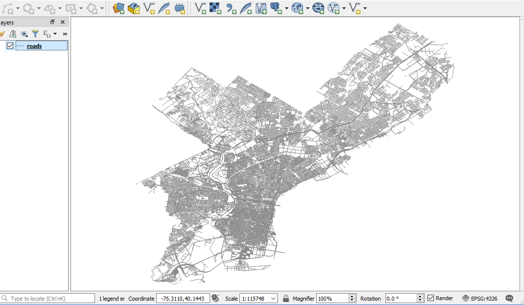 Figure 3.9 Sample QGIS map layout of Philadelphia roads
Now let's run the projection. - Type the following command (again this is a single command with the different parts separated by spaces):
ogr2ogr -t_srs EPSG:3857 -s_srs EPSG:4326 c:\data\PhiladelphiaBaseLayers\clippedAndProjected\roads.shp c:\data\PhiladelphiaBaseLayers\clipped\roads.shp
This one should run more quickly than the clip. - Start a new map in QGIS and add clippedAndProjected\roads.shp. It should be stretched a little more vertically than before.
Examining the parameters that you used for this command in tandem with the documentation, you'll notice that -s_srs is the coordinate system of the source dataset (EPSG:4326, or the WGS 1984 geographic coordinate system) and -t_srs is the target coordinate system (EPSG:3857, or the web Mercator projection). Because we're still using the ogr2ogr command, the final two parameters are the output and input dataset paths, respectively.
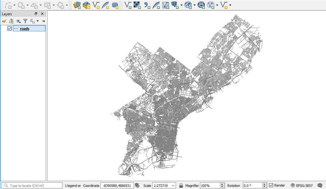 Figure 3.10 Sample QGIS map layout of Philadelphia roads in a different projection
You may be wondering, "How will I know which EPSG codes to use for the projections I need?" The easiest way to figure out the EPSG code for an existing dataset (which you'll need for the -s_srs parameter) is to add the dataset to a new map in QGIS and look in the lower-right corner of the screen as shown in Step 12 above. The easiest way to figure out the EPSG code for the target dataset (which you'll need for the -t_srs parameter) is to run the Save As command in QGIS and search for the projection. The EPSG code will appear as shown in Step 10 above.
Technical note for older versions of QGIS: If you are using a very, very old version of QGIS (prior to approximately version 2.14 Essen), you may see that the output dataset is shown in the Mercator projection, but the projection is reported in the lower-right hand corner as either EPSG:54004 or USER:100001 rather than EPSG:3857. In addition, if you add the original city_limits shapefile and the projected one to the same map project, you will notice a roughly 20km offset between the two polygons. QGIS needs a .qpj (QGIS projection file) to be associated with the shapefile in order to interpret the EPSG:3857 projection correctly. The ogr2ogr utility does not create the .qpj file by default because ogr2ogr is a general utility that is used with a lot of different programs, not just QGIS. To get a .qpj file, you could manually project a single dataset with QGIS into EPSG:3857, just like we did in the first set of steps above. This creates a shapefile that has a correct .qpj for EPSG:3857. Then copy and paste that resulting .qpj into your folder of output files that were projected with the ogr2ogr utility. You would need to paste the .qpj once for each shapefile and name it as <shapefile root name>.qpj. You would not have to modify the actual contents of the .qpj file because the contents are the same for any shapefile with an EPSG:3857 coordinate system.
The ogr2ogr utility is pretty convenient, but its greatest value is its ability to be automated. Let's clear out the stuff we've projected and see how the utility can clip and project everything in the folder. - Within your PhiladelphiaBaseLayers folder, delete everything in the clipped and clippedAndProjected folders. This gets you back to where you started at the beginning of the walkthrough. In order for these datasets to be successfully deleted, you will need to remove them from any open QGIS maps that may be using them.
- Go back to your command window and navigate to your PhiladelphiaBaseLayer folder using a command like the following: cd c:\data\PhiladelphiaBaseLayers
- Type the following command (as a single line) to clip all the datasets in this folder:
for %X in (*.shp) do ogr2ogr -skipfailures -clipsrc c:\data\PhiladelphiaBaseLayers\clipFeature\city_limits.shp c:\data\PhiladelphiaBaseLayers\clipped\%X c:\data\PhiladelphiaBaseLayers\%X
You can see the console messages cycling through all the datasets in the folder. Ignore any topology errors that appear in the console. This is somewhat messy data, and we have selected to skip failures.
Notice that this command is similar to what you ran before, but it uses a variable (denoted by %X) in place of a specific dataset name. It also uses a loop to look for any shapefile in the folder and perform the command. - Now navigate to the clipped folder using a command such as:
cd c:\data\PhiladelphiaBaseLayers\clipped
- Now run the following command (as a single line) to project all these datasets and put them in the clippedAndProjected folder:
for %X in (*.shp) do ogr2ogr -t_srs EPSG:3857 -s_srs EPSG:4326 c:\data\PhiladelphiaBaseLayers\clippedAndProjected\%X c:\data\PhiladelphiaBaseLayers\clipped\%X
You can add everything to QGIS to verify.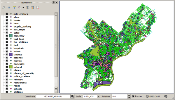 Figure 3.11 QGIS map showing output of the previous operations
Running the OGR utilities in a batch file
If you know that you'll be doing the same series of commands in the future, you can place the commands in a batch file. This is just a basic text file containing a list of commands. On Windows, you just save it with the extension .bat, and then the operating system understands that it should invoke the commands sequentially when you execute the file.
Try the following to see how you could use ogr2ogr in a batch file.
- Once again, delete all files from your clipped and clippedAndProjected folders.
- Create a new text file in any directory and paste in the following text consisting of five command lines (you may need to modify it to match your paths, especially your QGIS installation path which may use a different version name than 3.16.10):
cd /d c:\data\PhiladelphiaBaseLayers
set ogr2ogrPath="c:\program files\QGIS 3.16.10\bin\ogr2ogr.exe"
set GDAL_DATA=C:\program files\QGIS 3.16.10\share\gdal
for %%X in (*.shp) do %ogr2ogrPath% -skipfailures -clipsrc c:\data\PhiladelphiaBaseLayers\clipFeature\city_limits.shp c:\data\PhiladelphiaBaseLayers\clipped\%%X c:\data\PhiladelphiaBaseLayers\%%X
for %%X in (*.shp) do %ogr2ogrPath% -skipfailures -s_srs EPSG:4326 -t_srs EPSG:3857  c:\data\PhiladelphiaBaseLayers\clippedAndProjected\%%X c:\data\PhiladelphiaBaseLayers\clipped\%%X
Notice that these are just the same commands you were running before, with the addition of a few lines at the beginning to change the working directory and set the path of the ogr2ogr utility.
Batch files can use variables, just like you use in other programming languages. You set a variable using the set keyword, then refer to the variable using % signs on either side of its name (for example, %ogr2ogrPath%). Variables created inline with loops are represented in a batch file using %% (for example, %%X), a slight difference from the syntax you use when typing the commands in the command line window.
- Save the file as clipAndProject.bat (make sure there is no .txt in any part of the file name).
- In Windows Explorer, double-click clipAndProject.bat and watch your clipped and projected files appear in their appropriate folders.
Saving the data for future use
You will use this data in future lessons. Therefore, do the following to preserve it in an easy-to-use fashion:
- Create a new folder called Philadelphia, such as c:\data\Philadelphia. This folder will hold all your clipped and projected datasets for future reference.
- Copy all your datasets from the PhiladelphiaBaseLayers\clippedAndProjected folder into the Philadelphia folder.
- Following the techniques earlier in this walkthrough, use QGIS to save a copy of the PhiladelphiaBaseLayers\ClipFeature\city_limits.shp dataset in your new Philadelphia folder. Set the CRS as WGS 84 / Pseudo Mercator. (Remember that this layer was never originally projected, so you need to get a projected copy of it now.)
Walkthrough: Processing raster data with QGIS and GDAL
Now that you've seen QGIS and OGR in action with vector data, you'll get some experience processing raster data. For this exercise, we're going to start with a 30-meter resolution digital elevation model (DEM) for Philadelphia. I obtained this from the USGS National Map Viewer [13]. We'll use a combination of GDAL tools (some of them wrapped in a nice QGIS GUI) to make a nice-looking terrain background for a basemap. This will be accomplished by adding a DEM, a hillshade, and a shaded slope layer together. I have based these instructions on this tutorial by Mapbox [14] that I encourage you to read later if you would like further detail.
Download the Lesson 3 raster data [15]
Extract the data to a folder named PhiladelphiaElevation, such as c:\data\PhiladelphiaElevation. This will contain a single dataset called dem. In the interest of saving time and minimizing the download size, I have already clipped this dataset to the Philadelphia city boundary and projected it to EPSG:3857 for you. If you need to do this kind of thing in the future, you can use the Raster > Projections > Warp command in QGIS, which invokes the gdalwarp command.
- Launch QGIS and use the Add Raster Layer
 button to add dem to your map.
Don't add any vector layers right now. See the note at the end of this walkthrough if you are eventually interested in overlaying shapefiles with your terrain. - Create a hillshade by selecting dem in the table of contents and clicking Raster > Analysis > Hillshade. Save the hillshade as a TIF file named hillshade, and set the parameters as shown in the image below. Then press Run to execute the command.
Note that if you prefer the command line environment, you can make your future hillshades using the gdaldem hillshade command.
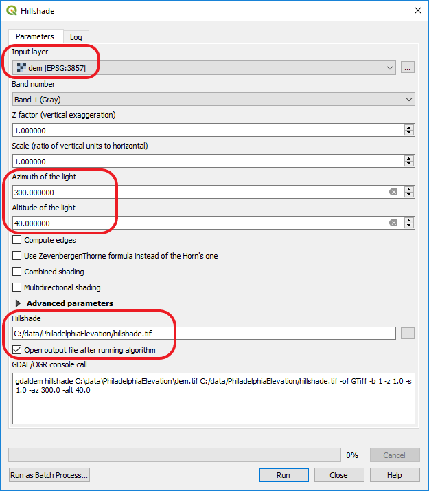 Figure 3.12 Hillshade tool GUI
 - Create a slope surface by highlighting your dem layer in the table of contents and clicking Raster > Analysis > Slope. Save it as a TIF named slope and keep the rest of the defaults. Each pixel in this surface has a value between 0 and 90 indicating the degree of slope in a particular cell.
Now let's shade the slope to provide an extra measure of relief to the hillshade when we combine the two as partially transparent layers. - Create a new text file containing just the following lines, then save it in your PhiladelphiaElevation folder as sloperamp.txt.
0 255 255 255
90 0 0 0
This creates a very simple color ramp that will shade your slope layer in grayscale with values toward 0 being lighter and values toward 90 being darker. When combined with the hillshade, this layer will cause shelfs and cliffs to pop out in your map. - Open your OSGeo4W command line window and use the cd command to change the working directory to your PhiladelphiaElevation folder.
- Run the following command to apply the color ramp to your slope:
gdaldem color-relief slope.tif sloperamp.txt slopeshade.tif
You just ran the gdaldem [16] utility, which does all kinds of things with elevation rasters. In particular, the color-relief command colorizes a raster using the following three parameters (in order): The input raster name, a text file defining the color ramp, and the output file name.
If you add the resulting slopeshade.tif layer to QGIS, you should see this:Now let's switch back to the original DEM and use the same command to put some color into it. Just like in the previous step, you will define a simple color ramp using a text file and use the gdal-dem colorrelief command to apply it to the DEM.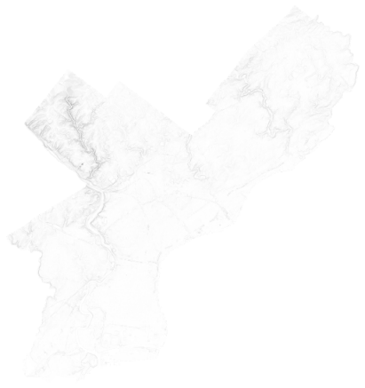 Figure 3.13 Hillshade results
 - Create a new text file and add the following lines (make sure your software doesn't copy it as one big line; there should be line breaks in the same places you see them here). Then save it in your PhiladelphiaElevation folder as demramp.txt.
1 46 154 88
100 251 255 128
1000 224 108 31
2000 200 55 55
3000 215 244 244
Note that the first value in the line is the elevation value of the raster, and the next three values constitute an RGB color definition for cells of that elevation. This particular ramp contains elevations well beyond those seen in Philadelphia, just so you can get an idea of how these ramps are created. I have adjusted the ramp so that lowlands are green and the hilliest areas of Philadelphia are yellow. If we had high mountains in our DEM, brown and other colors would begin to appear. - Run the following command:
gdaldem color-relief dem.tif demramp.txt demcolor.tif
When you add demcolor.tif to QGIS, you should see something like this:This looks good, but the No Data values got classified as green. We need to clip this again. This is a great opportunity for you to practice some raster clipping in QGIS.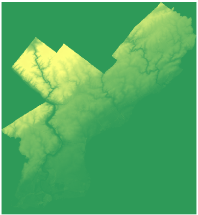 Figure 3.14 DEM sample
 - In QGIS, click Raster > Extraction > Clip raster by mask layer and set up the parameters as below. Make sure you clip demcolor to the city_limits.shp polygon from the previous walkthrough (it should be in PhiladelphiaBaseLayers\clipFeature) and to set the nodata value parameter to 0. Notice that at the bottom of this dialog box, the full gdalwarp syntax (used for clipping) appears in case you ever want to run this action from the command line. This can be a helpful learning tool! Make sure your output file name ends in ".tif" so that the -of GTiff option is added to the gdalwarp command.
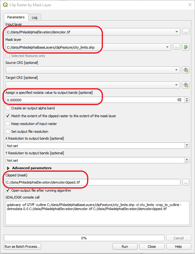 Figure 3.15 Clipper GUI
Now, let's add these together. - Create a new map in QGIS and add the clipped colorized DEM. Then add the hillshade with a 40% opacity. Then add the slopeshade with the 40% opacity. You should get something like below:
Now, play around with the transparencies to suit your liking. You can even re-run the colorization commands to apply different ramps.
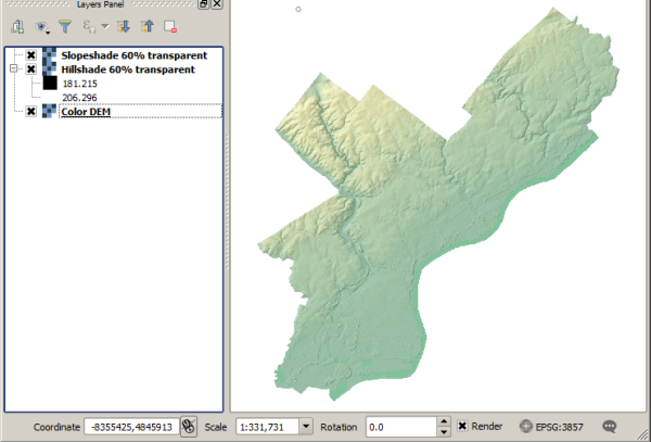 Figure 3.16 Sample map output in QGIS
This type of terrain layer, when overlayed by a few other vector layers, could act as a suitable basemap layer in a web map. In a future lesson, you'll learn how you could create tiles of this type of layer to bring into your web map.
Saving the data for future use
Just like in the previous walkthrough, you will copy your final datasets into your main Philadelphia data folder for future use.
Use Windows Explorer or an equivalent program to copy hillshade.tif, slopeshade.tif, and demcolorclipped.tif into the Philadelphia folder (such as c:\data\Philadelphia) that you created in the previous walkthrough.
Lesson 3 assignment: Prepare term project data and experiment with a GDAL utility
In this week's assignment, you'll get a chance to use some of your newfound QGIS and GDAL skills to prepare your term project data. This assignment has two distinct parts:
- Identify some data of interest (either from your workplace or your own personal interests) that you will use in the term project. The data must include thematic layers and layers suitable for creating a basemap from. So, even if in your final term project you are planning to use available 3rd party basemap options, please obtain some additional data sets that can serve as a background for your thematic data. If necessary, you can create some of the layers yourself.
Download these datasets and get them into the desired format and scope using FOSS tools. Also, project them into the EPSG:3857 projection (one of the tools we'll use later requires it).
Then write 300 - 500 words about your choice of these datasets, also describing the methods and tools you used to process them. Indicate which of the datasets will act as the thematic layer in your eventual web map.
Include relevant screenshots, including an image of your final datasets all shown together in QGIS. Don't worry too much about cartography yet; just show me that you obtained and projected the datasets.
Please note that in your practical workday, you should use whatever tools are easy and available to wrangle your data (including proprietary software); however, in this assignment, I would like you to use FOSS, so you can get some practice with it.
Submit this portion of the assignment to the Lesson 3 (part 1) drop box on Canvas.
- Investigate a GDAL (or OGR) command that you might find useful in your day-to-day work. On the Lesson 3 assignment (part 2) forum on Canvas, post an example of successful syntax that you used with this command, along with "before" and "after" screenshots showing how a dataset was affected by the change. This can be a command that you used in the assignment above, but not one of the commands detailed in the lesson walkthrough. Please make sure to briefly explain the parameters used in your command, unless their meaning is extremely obvious (like input and output file names).
The following pages list the available commands. Although the OGR list looks short, be aware that ogr2ogr has many available parameters and can do a variety of things:
GDAL raster programs [20]
OGR vector programs [21]