Project 1: Density Surface Options
Option 1: Points at Polygon Centroids
The first option is to make a set of points, one for each polygon in our 2002 voting data, and to use these to represent the distribution of the vote that might be expected in 2004. This approach assumes that it is close enough to assign all the voters in each polygon to a single point in the middle of that polygon.
This is a two-step process, creating a point layer, and converting the point layer to a raster.
To make the point layer:
- Open the Geoprocessing pane from Analysis-Tools. Then search for the Feature to Point tool with the search bar and launch it. Select tx_voting108 as the 'Input Features' and specify a name for the point layer to be produced. You may also optionally choose to force the points to lie inside the polygons.
NOTE: this is a step that requires an Advanced level license. Your student license should be an Advanced level license.
HOWEVER... because this is Lesson 1, we have provided the results of this step (with the 'force inside' option not selected), in the layer tx_voting108_centers layer.
By whatever means you arrive at a point layer, make sure you understand what is going on here. In particular, check to see if all polygons have an associated center point. Are all the 'centers' inside their associated polygons? (If not, why not?)
Once you have the point layer, you can make raster layers (one for Republican voters, and one for Democratic voters) as follows:
- Search for and launch the Point to Raster tool.
- Select the centroids layer you just made as the Input Features and either REP or DEM as the 'Value field' (you need to make one surface for each attribute).
- Also specify a name for the new raster surface to be created (reps_point or dems_point as appropriate).
- Use 'SUM' as the 'Cell assignment type' (why?).
You will get a raster layer with No Data values in most places, and higher values at each location where there was a point in the centroids layer.
Option 2: Density Estimation from Points
The second option is to use kernel density estimation (which we will look at in more detail in Lesson Three) to create smooth surfaces representing the voter distribution across space. This method requires you to choose a radius that specifies how much smoothing is applied to the density surface that is produced.
The steps required are as follows:
- Search for and launch the Kernel Density tool
- Set 'Input data' to the point centers layer (as made in the previous method). For the 'Population field' select REP or DEM (you will be doing both anyway). Set the 'Search radius' to 20,000 [or another value you feel is appropriate for modelling voter distribution], and 'Area units' to 'Square Kilometers'. You should also specify a name to save the output to (I suggest reps_kde, or dems_kde, as appropriate). Then run the tool.
The search radius value here specifies how far to 'spread' the point data to obtain a smoothed surface. The higher the value, the smoother the density surface that is produced.
If you encounter problems, post a message to the boards, and also check that the map projection units you are using are meters (the easiest way to check this is to look at the coordinate positions reported at the bottom of the window as you move the cursor around the map view).
When processing is done, ArcGIS Pro adds a new layer to the map, which is a field of density estimates for voters of the requested type. You should repeat steps 1 and 2 to get a second field layer for the other political party, making sure that you calculate both fields with the same parameters set in the Kernel Density tool.
NOTE: If you have changed the Analysis Environment Cell Size setting from the suggested 1000 meters, then the density values you get are correct, but when it comes to summing them (in a couple more steps' time), they will not produce correct estimates of the total number of votes cast for each party. This is because the density values are per sq. km, but there is not one density estimate for every sq. km. For example, if you set the resolution to 5000 meters, then there will be one density estimate for every 25 sq. kms. To correct for this, you need to use the raster calculator to multiply the density surface by an appropriate correction factor: in this case, you would multiply all the estimates by 25.
NOTE 2: If you are running ArcGIS Pro 2.8 or later, there has been a change to how the KDE tool works. To produce the expected result, you will need to change the processing extent in the Environments tab to either the same as the 'tx_voting108' layer or to the 'union of inputs'. Otherwise, you'll see a result that appears to include only North Texas.
Option 3: Assumed even population distributions
The third option is to assume that voters are evenly distributed across the areas in which they have been counted. We can build a surface under that assumption and base the final estimated votes in the new districts based on that. This method takes a couple of steps and creates two intermediate raster layers using the Spatial Analyst extension on the way to the final estimate.
A number of steps are required:
- Search for and launch the Polygon to Raster tool and use it to make new raster layers from the OBJECTID, REP and DEM fields of the tx_voting108 layer. You will need to run the tool three different times, to make three different layers. The default cell size should be 1000 meters. You should specify a sensible (and memorable) name for each raster layer you create (reps, dems, ids are what I used).
- For the raster layer made from the OBJECTID field, you need to count the size of each area, in raster cells. Search for and launch the Lookup tool from the Spatial Analyst toolbox. Choose your ids raster as the 'input raster', Count as the 'lookup field', and name your output layer ids_count. This will produce a new raster that stores the number of pixels in each voting district. Because you set the cell size to 1000 meters, this is also effectively an area in square kilometers.
- Now, search for and launch the Raster Calculator tool. Then, for each party, use the Raster Calculator to calculate the number of Republican and Democratic Party voters per raster cell (i.e., per square kilometer) as shown in Figure 1.4. Notice that we used the int function to make sure that we have integers because votes only exist in integer quantities -- there are no partial votes! Make sure you build the expression by clicking on items rather than typing. This will make it less likely that you get a syntax error.
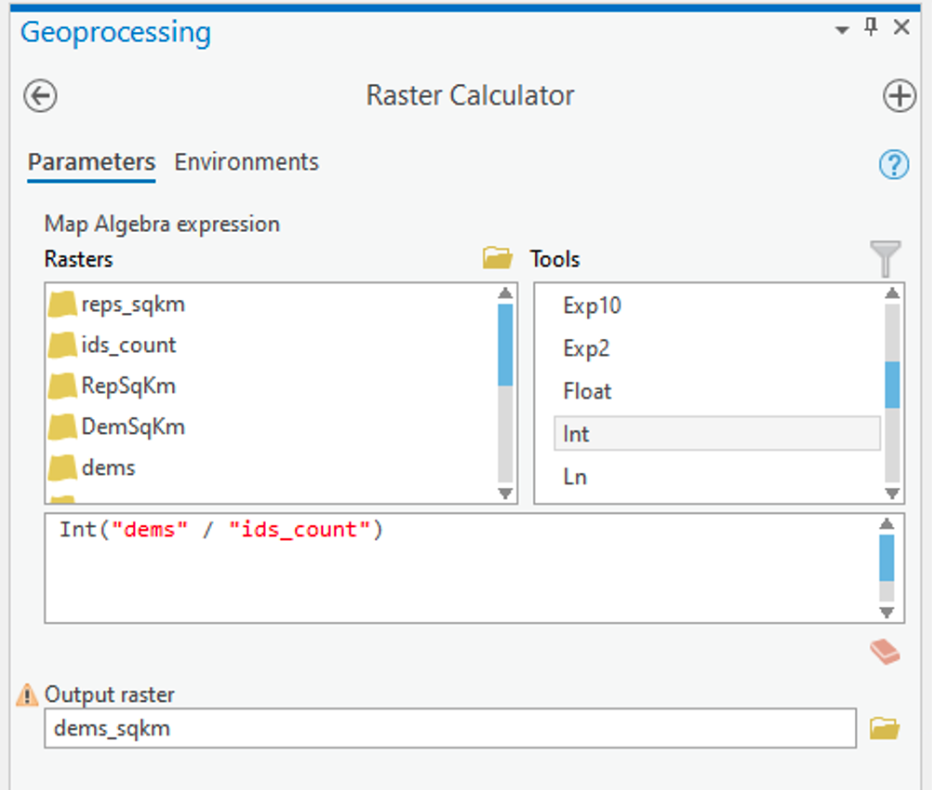 Figure 1.4: Raster CalculatorClick for a text description of the Raster Calculator Example image.The raster calculator expression should be the name of the democrat raster layer divided by the result of the lookup tool. Notice that we used the int function to make sure that we have integers because votes only exist in integer quantities – there are no partial votes! The output parameter should set the name of the output to something informative.Credit: Griffin
ArcGIS Pro will think about things for a while and should eventually produce a new layer (in this case called dems_sqkm). This layer contains in each cell an estimate of the number of voters of the specified party in that cell.