Lessons
This is the course outline.
Lesson 1: Introduction to GIS-T
Learning Outcomes
What will we learn?
By the end of Lesson 1, you should be able to:
- characterize the relationship between GIS and transportation and explain why GIS-T is such an active field;
- discuss some of the challenges and opportunities for GIS-T in the 21st century;
- list some modes of transportation and discuss the meaning and significance of modal competition, modal shift, and containerization;
- state the mission and describe some of the current initiatives of the U.S. Department of Transportation (USDOT);
- describe some of the geographic areas the Census Bureau uses to aggregate and disseminate data.
1.1 Introduction to GIS-T
Among the many areas and disciplines to which GIS has been applied, transportation has been particularly fertile ground, and the development of specialized GIS applications has been an area which has seen a lot of activity. This important interdisciplinary field is commonly referred to as GIS-T. The significance of this field is evidenced by the fact that there are two conferences devoted to it, one annual and one biennial. Each year the American Association of State Highway and Transportation Officials (AASHTO) sponsors the annual GIS for Transportation Symposium [1]. The symposium draws over 400 registrants from federal, state, and local government and the private sector. The Urban and Regional Information Systems Association (URISA) sponsors a conference called GIS in Transit [2]which is held every other year. The 10th GIS in Transit conference was held last year.
A key reason that GIS-T is so important is that transportation is a huge industry upon which many other industries depend. In 2015, the federal government spent 85 billion dollars on transportation-related initiatives. That represented 2.22% of our total federal budget for 2015. The National Priority Project (NPP) website [3] presents some interesting charts which put federal transportation spending in perspective.
Additional Learning
In their own words, the NPP “is a national non-profit, non-partisan research organization dedicated to making complex federal budget information transparent and accessible so people can prioritize and influence how their tax dollars are spent.” Their website also offers a number of very educational videos [4] if you’d like to understand our national budget, deficit, and debt.
In addition to federal dollars, there are many billions of state and local dollars spent on transportation. If you want to see how states are using transportation dollars, the Track State Dollars website [5] gives you access to data for each state.
In the U.S., federal agencies have helped to promote GIS use for transportation analysis purposes through geospatially-enabled initiatives such as the U.S. Census Bureau’s TIGER program and the Federal Highway Administration’s Highway Performance Monitoring System (HPMS). Software vendors have continually updated and improved their GIS products to include additional GIS-T functionality and tools. Today, GIS-T is an integral part of transportation operations around the world.
The natural synergy between GIS and transportation is at least in part due to the fact that transportation is inherently spatial, and while it’s true that GIS plays an important role in transportation, one can also argue that transportation plays an important role in GIS. Transportation features are frequently included on maps for context and orientation even when the fundamental purpose of the map has little or nothing to do with transportation. Take a few minutes to review this recent blog [6] from GeoSpatial World which briefly examines some important applications of GIS to transportation. In this course, we'll cover these application areas as well as many others.
1.2 Overview of the Transportation Industry
Broadly speaking, the field of transportation is concerned with the transport of people and goods. To appreciate the value that GIS brings to transportation it is necessary to develop an understanding of the various forms of transportation that exist and also the types of activities and problems which those in the field need to address.
Transportation Modes
The different ways that people and freight can be transported are referred to as transportation modes. There are many different modes of transportation, and they can be differentiated and categorized in a number of ways. At a high level, we can divide transportation into the categories of air, land, sea, and space. We could further divide the land-based transportation into road, rail, pedestrian, bike, and pipeline, although one might rightfully argue that pipelines can run under the sea. Transportation modes are not always mutually exclusive and the specific modes we talk about often depend on the situation at hand. There have been many GIS applications which have been designed for a specific mode or for a group of closely related modes.
Transportation Processes and Activities
Just as we can categorize transportation according to the many modes of transportation which exist, we can think about transportation in terms of the many processes and activities which are performed in order to manage transportation infrastructure, vehicles, and operations. Some of these processes cut across modes and others are specific to a single mode or a few modes. These processes and activities include:
- infrastructure monitoring and maintenance;
- transportation planning and transit planning;
- property acquisition and management;
- vehicle tracking and logistics;
- highway safety analysis and improvement;
- traffic monitoring, modeling, and mitigation;
- screening projects for environmental impacts;
- dissemination of travel information to the public;
- reporting data to government agencies to secure funding;
- mobile data collection;
- routing and permitting of oversize overweight vehicles.
GIS-T plays an important role in enhancing the manner in which transportation organizations accomplish these processes and activities and, in some cases, allow organizations to perform functions which would simply not be possible without spatial technologies. GIS-T applications support evaluation of different scenarios, provide objective data for decision-making purposes, and promote the visualization of conditions.
GIS-T Techniques and Tools
GIS-T utilizes many mainstream geospatial tools and methods but it also employs a number of techniques which were borne out of the specialized needs of the transportation industry. These include:
- Conflation
Conflation is a technique used to bring together adjacent or overlapping datasets which were collected at different times and have different levels of accuracy and precision. While the process of conflation in GIS is frequently applied to transportation networks, conflation can also be used to combine other types of features. - Network Analysis
A roadway network is comprised of roads and intersections. In network terminology, the intersections are referred to as nodes, and the streets which connect the nodes are called edges. GIS-T commonly employs network analysis techniques to roadway networks to solve common transportation-related problems such as finding the best route between two points or determining the service area around a specific location (i.e., the area within which someone could reach the location of interest in a defined period of time). - Linear Referencing Systems
Linear referencing systems (LRS) are used to spatially reference the location of assets (e.g., bridges), occurrences (e.g., crashes), and roadway characteristics and administrative data (e.g., speed limits) by specifying the distance along a linear feature in a roadway network. Collectively, these attributes of a roadway are referred to as events. In this course we'll only consider the application of an LRS to roadway networks, they can be used in any linear network including pipelines and hydrologic networks. - Dynamic Segmentation
Dynamic segmentation is closely linked to LRS. In dynamic segmentation, we take the roadway events which are linearly referenced along roadways and transform them on the fly into spatial features. Taken together, LRS and dynamic segmentation allow us to effectively manage and utilize the myriad of attribute information associated with roadway networks. We will explore these techniques in detail in Lesson 6.
We will learn more about these techniques in upcoming lessons.
1.3 Getting to Know a Transportation Organization
This week, you’ll take some time to get to know perhaps the most significant transportation organization in the United States, the U.S. Department of Transportation (USDOT). The USDOT (established in 1966) is a cabinet-level department within the U.S. government which employs about 55,000 people and is responsible for maintaining and advancing the nation’s transportation systems and infrastructure.
A key function of the USDOT is to develop programs which implement transportation-related statutes. One of the most important statutes the USDOT is tasked with implementing relates to the funding of surface transportation. The latest surface transportation statute is known as the Fixing America’s Surface Transportation (FAST) Act, which was signed into law by President Obama in December 2015.
The USDOT is comprised of a number of operating administrations and bureaus, each of which specializes in a specific area of transportation. Some of these divisions, along with the area of transportation they are responsible for, are listed below:
- Federal Highways Administration (FHWA)
Specializes in highway transportation - Federal Transit Administration (FTA)
Provides financial and technical assistance to public transit agencies - Federal Aviation Administration (FAA)
Regulates all aspects of civil and commercial aviation and operates a national system of air traffic control and navigation - Federal Railroad Administration (FRA)
Enforces rail safety regulations and administers railroad assistance programs - National Highway Traffic Safety Administration (NHTSA)
Specializes in reducing vehicle-related crashes
We’ll take a closer look at some of these USDOT divisions in later lessons.
Spend some time looking at the USDOT’s website [7] and try to learn some more about the organization and some of their current initiatives and activities. Also, spend some time learning about the Smart City Challenge which the USDOT kicked off in December 2015. This challenge was designed to promote innovative solutions to some of the biggest challenges our cities face and offered $50 million to the winning city, $40 million of which came from the USDOT and $10 million from a private partner. Here is a video where the USDOT provided information to city mayors across the county. (Note: the presentation doesn't begin until about 10 minutes into the recording and you may want to skip ahead to the 18-minute mark when former Transportation Secretary Anthony Foxx begins to speak).
Video: Smart Cities Webcast (25:14)
KEVIN: Good afternoon. My name is Kevin Monroe, Deputy Assistant Secretary for governmental affairs here at the US Department of Transportation. Now, I want to welcome and thank you for joining us today for a webcast on the Smart City Challenge. Secretary Foxx will be joining us shortly, but right now I'd like to take the opportunity to introduce my colleague, Mark Dowd, Deputy Assistant Secretary for Research and Technology. He will tell us more about the Smart City Challenge. Mark.
MARK: Hi, welcome. I'm going to take you through some of the details for the Smart City challenge to get you oriented as to what we're looking for. We'll be hearing from the secretary shortly. He is extremely excited about this challenge. As a former mayor, he is looking forward to hearing from his fellow mayors as to how to solve the issues that we identified in "Beyond Traffic".
Beyond Traffic, narrative identified the issues of moving people and moving goods, and so we decided that it would be good to reach out to cities and encourage them to put forward their most creative ideas on how to solve those problems using technology and innovation.
I want to take you through a little bit of the schedule. We have two phases: phase one and the most important part is the deadline coming up on February fourth. We are looking for cities to put forward their high-level, thirty-page ideas as to how to solve these issues using innovation and technology. The second phase when we down select to 5 will be we will move through the process of awarding the five finalists 100,000 dollars and selecting the finalist who will receive the 50 million dollars.
I think I'll take you through a little bit of what we're looking for. We are looking for a medium-sized city, although we accept applications from all cities. This is generally what we're looking for, from in terms of particularity. We're looking for a population between 200,000 and 850,000 using 2010 census data, a dense urban population that's typical for a medium-sized city. We're looking for leadership in the city that is committed to carrying this through for the three years of the program. There are a number of different aspects of smart cities that people talk about. We thought we'd talk a little bit about from a smart city perspective what we're looking for in the transportation sector. There are a number of technologies on the left-hand side that will feed into the solutions and then, on the right-hand side are the benefits that we're looking for. We tried to lay out our vision of what of what this would look like and we tried to do it with 12 vision elements that are identified in the notice of funding opportunity. The highest priority is the technology elements that are urban automation, connected vehicles, and sensor-based infrastructure. The second level priority is the innovative approaches to urban transportation and these include the sharing economy, Open Data, urban analytics, connected involved citizens, and smart strategic business partnerships. Lastly are the other three smart city elements that are in each architecture and standards, smart land use, and low-cost, efficient ICT.
In your thirty-page, high-level application, we're looking for certain similarities in all the applications that we lay out what we're looking for in our narrative description. The evaluation criteria which will drive a lot of the narrative that includes a lot of what we talked about earlier, which is including population size, etc.
I think is important to take us through a couple of the critical deadlines that we're looking for. The applications are due on February 4th at 3 p.m., and then once we receive the application, we'll go through a fairly rigorous procurement process to down select to the five finalists. We'll announce the finalists in March 2016. Soon thereafter, we will issue $100,000 to each of the finalists to help them get their applications in in good form to compete for the final award. The final award will be issued in June 2016 to the winning city.
I'm sure you have additional questions or concerns and we'll have various opportunities for you to interact with the department on how to solve those problems and those issues that you have. We have an in-person Smart City forum that is on December 15th here at the Department of Transportation between nine o'clock and four o'clock. We have about 350, 400 people already signed up for this in-person meeting and then following that we'll have a number of technical advisories. We'll do data, architecture, and standards on December 16th, connected vehicles and automation December 17th. We'll discuss sharing economy, user-focused mobility on December 18th, and then we'll help you navigate the smart city challenge application process we'll be out shortly with that announcement.
I'm sure you have questions. Please don't hesitate to send them to smartcitychallenge@dot.gov [8], and we will continue to update our website with additional dates and additional information at transportation.gov/smartcity.
BRYNA: Mark, thank you very much. Stay here. Hi, my name is Bryna Helfer. I'm the Deputy Assistant Secretary for Public Engagement and we just wanna, Mark, I guess I we just want to go back. We've been getting some questions about the elements, and I was wondering if you might just spend a little bit of time talking about your vision for the elements and what goes into some of these elements. If you could, that would be awesome, thanks.
MARK: Sure. So, in urban automation oftentimes when people talk about automated vehicles they talk about it in a singular, linear sense. We actually think that urban automation goes beyond just the urban, beyond the automated vehicle. The moving of goods through automation, the moving of people through automation, and how it interacts with the sharing economy, how it interacts with connected vehicles, and how it interacts with this sensor-based infrastructure that's either in the city already or is being developed by the city. So, the important part about the technology elements is that we're not looking for just another connected vehicle pilot. We're not looking for just an automation pilot. We're looking for how these different technologies work together. The innovative approaches, if you go through them, we have a very lengthy description in the notice of funding opportunity as to what they all mean. But if you look at the connected and involved citizens, it's important that we get through urban delivery and logistics, etc. Finally, the Smart City elements, the smart land use, etc., are very, are described. And those are key elements.
Wanted to introduce Secretary of Transportation now who will talk a little bit about the Smart City Challenge.
SECRETARY FOXX: Hi Everyone, thank you, Mark, and thank all of you so much for joining today's webcast. As you know, yesterday we launched our Smart City Challenge targeting mid-size cities. This is an opportunity for mayors and city leaders to define what it means to be a smart city when it comes to transportation. We're asking cities to submit proposals by February 4th, and our goal will be to narrow the proposals down to five finalists by May and announce the winner in June; the winner will then receive up to forty million dollars to implement their proposal. That's not all. As Mark has probably alluded to already, our partner in this effort, Vulcan, is offering an additional ten million dollars to the winning city. And our hope is that cities will see this as an opportunity to partner with firms like Vulcan, and other innovators that can help them re-imagine their transportation systems.
Let me just talk some about why we are doing this. First of all, we don't have a top-down transportation system in the U.S., we have a bottom-up system, and while we are grateful that Congress passed a five-year transportation bill last week, our national vision for transportation is still in some ways stuck in the 20th century when it comes to thinking about technology, innovation, and the kind of inputs that mayors and local officials think about all the time when it comes to how to integrate transportation and quality of life and, of course, protecting our environment and so many other issues. So, our department is working hard on the national level to create policies and programs and practices that help make it easier for local and state decision-makers to do these things. We're trying to reposition government so we can help you solve problems at the local level. We also want to increase our ability to rapidly absorb technology in the transportation space so we can do things that previous generations could only imagine. So, we're imagining things like connected and autonomous vehicles that practically eliminate crashes. And we're imagining this technology interacting with wired infrastructure to eliminate traffic jams as well, but we're not only imagining it happening, we're making it happen. We're moving quickly to require all new cars to be equipped with vehicle-to-vehicle technology. And, as part of this effort, we also launched a pilot program to demonstrate connected vehicles in three US cities, including New York. We're updating our policy position on autonomous vehicles and we're working to integrate unmanned aircraft into the National Airspace. We even have hired our first data chief data officer. So, we've pushed as hard as we can and will keep pushing at the national level, and now we're hoping to incentivize you at the local level to work just as hard. And, ultimately, we know that the best laboratory we have for emerging innovation and technology is where it is most needed, which is in our cities.
Another forward-looking thing we did was to look at our transportation system over the next 30 years, and this bears directly on all of you on the call. Our report "Beyond Traffic" tells us that we're gonna add seventy million more people to our population over the next thirty years, and it's also telling us that our cities will absorb most of this growth. This is part of the reason it's been said that the 20th century will not be dominated by countries, but it will, in fact, be dominated by the rise of cities and the rise of urbanization in regionalism. Along these lines, the entire world is now having a conversation about smart cities which is really a conversation about what our cities should look like in the future, and now our cities will need to show us. In this challenge, all of you will help define what a smart city is. So, rather than be prescriptive, we want you to be bold. We're asking you to develop your own unique vision, your own unique partnerships, your own unique blueprints, for building the city of the future, and we're putting the ball in your court in giving you the opportunity to demonstrate to the world what a fully integrated, forward-looking transportation network looks like. I want to say this because I know that many of you have been working on your community's vision statements and plans and land use strategies and all sorts of things. This challenge is an opportunity to bring all that together and to make progress. So to everyone joining us for this, I want to assure you that this is not only the beginning of our outreach process; we will continue making outreach happen over the next several weeks. In fact, tomorrow we'll host a smart city forum. Actually, I'm sorry, December fifteenth we will host a smart city forum, and we encourage folks to join us in person, but will also have a virtual option available as well. As I say, we'll have more webinars in the coming weeks. So, I'm looking forward to seeing the proposals that come forth. I'm also looking forward to working with you, all of you to push the boundaries of what is possible. And, with that, I'll turn it back to my team to give you more details and answer any questions you have and with that, thank you very much. It's been great to be with you.
KEVIN: Thank you Secretary Foxx and thank you, Mark Dowd. As the secretary just mentioned, I want to remind you that you can sign up online for the December 15th in-person Smart City forum here at USDOT. He did mention that there will be an online option also. Please go to www.transportation.gov/smartcity [9] that's www.transportation.gov/smartcity [9]. Ladies and gentlemen, thank you very much again for joining us today.
Video: #SmartCityPitch: Columbus (2:35)
ON SCREEN TEXT: In Columbus, we've built an unprecedented culture of collaboration. We've knocked down silos, and built up partnerships to become the Midwest's fastest-growing city. #1 in job growth #1 in population growth. Our culture of collaboration is the Columbus way. It is how $50 million becomes $140 million. We will set the pace for smart city transformation. We will connect hard-working people to jobs. We will lift a low-income community out of poverty. Give students of all ages unprecedented access to education. Give more expectant mothers access to prenatal care, and get more children to Pre-K. Through collaboration, we get things done. By sharing data, and leveraging advanced analytics, we will clear congestion and improve safety like never before. We will demonstrate how a city can leap ahead. You see, we know how to lead (fastest growing city for startup activity in 2015), to collaborate (#1 metro for job growth in the Midwest), to set a bold vision (lead the country in smart mobility), and best of all we know how to deliver results. So, let's transform Columbus. Let's build a connected, cutting edge, sustainable, smart city. Smart Columbus will move America forward. We're ready. All of us. #smartcolumbus
The winner, announced in June 2016, was Columbus, Ohio. I think you’ll agree that their winning pitch (see above) exhibited an impressive use of multimedia.
Take a look at these links to see what's happened since the award was made in June 2016:
- The USDOT published a report [11] summarizing the lessons learned thus far.
- The city of Columbus is maintaining a list of the Smart City projects [12] which are planned or underway.
- Learn how Columbus turned the $50 million award into $500 million [13] by leveraging private investment (also check out the video at the top of the page to see some of their innovative ideas).
1.4 Getting to Know Each Other
One of my goals for this course is to promote meaningful interactions between all of us as we cover topics in GIS-T over the next 10 weeks and to lay the framework for building relationships which will extend beyond the end of the course. Throughout the course, you will have the opportunity to get to know your classmates and me a little better. As a first step, you will create a video autobiography so we can begin to get to know you. In later lessons, you will spend time in one-on-one video chats with your classmates getting to know each other better.
1.5 Webinar for Next Week
Speaker
Our next webinar will be with Mr. Michael Ratcliffe. Michael is Assistant Division Chief for Geographic Standards, Criteria, Research, and Quality in the Census Bureau’s Geography Division, where he is responsible for geographic area concepts and criteria, address and geospatial data quality, and research activities. During his tenure at the Census Bureau, he has worked in both the Geography and Population Divisions, on a variety of geographic area programs, including urban and rural areas, metropolitan and micropolitan statistical areas, and other statistical geographic areas, and has led staff engaged in product development and dissemination. In addition to his work at the Census Bureau, he is an adjunct professor at George Washington University, where he teaches Population Geography. Prior to that appointment, he was an adjunct instructor at the University of Maryland-Baltimore County. Mr. Ratcliffe holds degrees in geography from the University of Oxford and the University of Maryland.
Geographic Areas Used by the Census Bureau
The Census Bureau defines many different geographic areas which can be used to organize and aggregate data. The areas the Census Bureau uses can be divided into those which are legally defined and those which are not. The Census Bureau refers to non-legally defined areas as statistical areas.
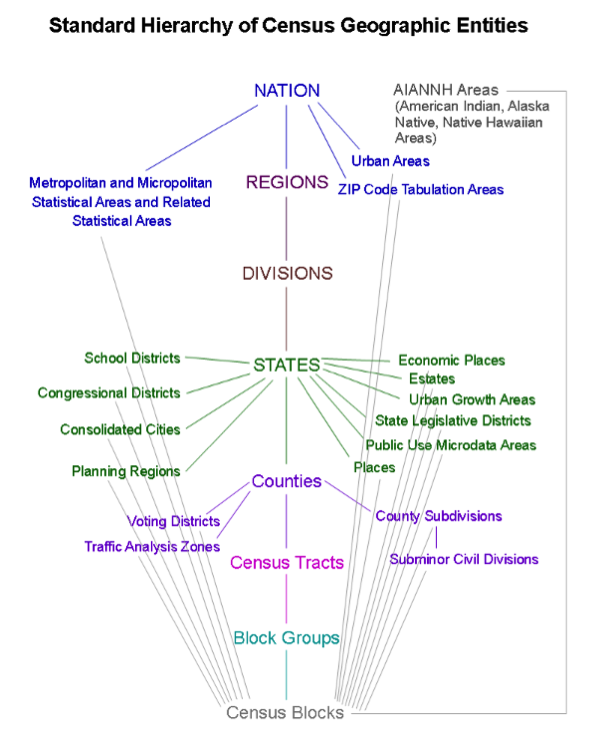
Nation
Metropolitan and Micropolitan Statistical Areas and Related Statistical Areas
Urban Areas
ZIP Code Tabulation Areas
Regions
Divisions
States
School Districts
Congressional Districts
Consolidated Cities
Planning Regions
Economic Places
Estates
Urban Growth Areas
State Legislative Districts
Public Use Microdata Areas
Places
Counties
Voting Districts
Traffic Analysis Zones
County Subdivisions
Subminor Civil Divisions
Census Tracts
Block Groups
Census Blocks
AIANNH Areas (American Indian, Alaska Native, Native Hawaiian Areas)
Metropolitan and Micropolitan Statistical Areas and Related Statistical Areas
Urban Areas
ZIP Code Tabulation Areas
School Districts
Congressional Districts
Consolidated Cities
Planning Regions
Economic Places
Estates
Urban Growth Areas
State Legislative Districts
Public Use Microdata Areas
Places
Voting Districts
Traffic Analysis Zones
County Subdivisions
Subminor Civil Divisions
1.5 Summary of Lesson 1
In this lesson you:
- briefly examined the important role GIS plays in the field of transportation and learned about the manner in which GIS-T is evolving in the 21st century. \
- learned something about transportation modes and the concepts of mode competition, mode shift, and containerization.
- spent some time learning about the role of the USDOT in the transportation industry. .
- aquainted yourself with the speaker and general topics for next week's webinar.
- took the first step in getting to know each other by creating a video autobiography which will serve to introduce you to the rest of the class.
Questions and Comments
If there is anything in the Lesson 1 materials about which you would like to ask a question or provide a comment, submit a posting to the Lesson 1 Questions and Comments discussion. Also, review others' postings to this discussion and respond if you have something to offer or if you are able to help.
Lesson 2: Roadway Centerline Data
Learning Outcomes
What will we learn?
By the end of Lesson 2, you should be able to:
- compare and contrast different sources of roadway data which are available;
- compare the ways Google and OSM enlist the help of volunteers to improve their roadway data;
- describe the characteristics of the TIGER/Line shapefiles and OSM data;
- discuss the use of Census data for transportation planning;
- explain the purpose of Section 106 of the National Historic Preservation Act (NHPA) and describe how it impacts transportation projects;
- list some details about your classmates based on your review of their video autobiographies.
2.1 Roadway Data Sources Used in GIS-T
Roadway data are fundamental to GIS-T and many of the most important transportation modes (e.g. highway, transit, bike). Many GIS functions and analyses rely on it including geocoding and network analysis, both of which we’ll take a close look at in the next few lessons. Roadway data also play an important role in mapping and visualization for many GIS applications.
There are a number of commercial and public sources of street data and services which are available. Some are public and freely available, and others are commercial. In this lesson, we’ll take a look at some of the most widely used sources of street data.
Public Sources
TIGER Data
TIGER is a data source produced and published by the U.S. Census Bureau. These data include street data which can be used to perform geocoding or to produce a street network. TIGER data were used as a “seed” for many of the other roadway data sources, both public and commercial. We will take a closer look at TIGER data later in this section.
OpenStreetMap (OSM)
OSM is a rapidly growing Volunteered Geographic Information (VGI) project which got its start in 2004 and is sponsored by the OpenStreetMap Foundation. For U.S. roads, OSM initially used TIGER Line files but many updates have since been made based on input from its volunteer community which is now over a million strong. In some parts of the world, OSM data are as good, or nearly as good, as its commercial counterparts.
Agency-Generated
State-level transportation agencies have long maintained road centerline networks as well as additional networks for other modes. They have been improved greatly in accuracy and precision, and agencies are increasingly adding local and private roads and associated data. Much of this latter impetus is due to increased federal requirements for data collection and reporting. In most cases, these networks are the most complete and accurate product for network features and associated attributes for any given state.
Transportation for the Nation (TFTN)
TFTN is an evolving governmental initiative from the National States Geographic Information Council (NSGIC) and USDOT that originated in 2008. TFTN will initially be a road centerline dataset that may replace overlapping federal efforts and products. A set of centerline datasets has been created as part of state DOT submittal requirements for FHWA’s Highway Performance Monitoring System (HPMS). The next step is to try and join these across state lines.
Commercial Sources
TomTom / Tele Atlas
Tele Atlas was founded in 1984 and was acquired by TomTom in 2008. Tele Atlas data was primarily collected from its own mapping vans. The company’s road products are decreasing in importance and usage.
Nokia / NAVTEQ / HERE
Founded in 1985 and acquired by Nokia in 1991, NAVTEQ (now renamed HERE) operates independently and partners with third-party agencies and companies to provide its networks and services for portable GPS devices made by Garmin and others, and Web-based applications including Yahoo! Maps, Bing Maps, Nokia Maps, and MapQuest.
ESRI StreetMap and StreetMap Premium
ESRI does not produce road data directly but instead acquires it from HERE, TomTom, and others and repackages it. ESRI StreetMap covers North America and is part of Data and Maps which is included with ArcGIS. StreetMap premium has more current data than StreetMap and also has coverage for Europe.
Google has become a major provider of mapping services. Google doesn’t make its street data available directly but instead uses it to provide services. These services are provided through products such as Google Maps, Google Earth, and various APIs. In 2008, Google released a tool called Google Map Maker to encourage individuals to submit or correct feature information. This is similar in concept to the manner in which OSM derives much of its data. Google retired Map Maker in 2017 in favor of its "Local Guides [15]" program. As a "Local Guide," you can contribute reviews of businesses or places, upload photos and suggest a new place. Recently, they also began to add capabilities to allow users to report issues with roadway geometry and missing roads. Local Guide contributions are all made directly in the Google Maps interface. Take a look at these comparisons between OSM and Google in regards to the services [16] they provide and their user contributions [17] programs. One should note these comparisons are published on the OSM Wiki site so they may be a bit biased.
Also, check out this map comparison tool [18] made available by Geofabrik, an organization who promotes OSM and provides a portal for downloading OSM data extracts. Select an area you are familiar with, and compare the OSM map, the Google map, and the HERE map.
2.2 Exploring TIGER and OSM Data
In this section, we'll take a closer look at two of the most extensive sources of publicly available roadway data: TIGER and OSM.
The TIGER database was first created in preparation for the 1990 decennial census. In creating TIGER, not only did the Census Bureau produce the first nationwide map of roadways, it also incorporated topographical context which defined the relationship between road features as indicated in its name: Topologically Integrated Geographic Encoding and Referencing database.
In addition to the TIGER spatial database, the Census Bureau also created a Master Address File (MAF) which is a database of all known living quarters in the U.S. The MAF contains about 300,000 addresses which are identified as location addresses, mailing addresses or both. In addition, the MAF contains a record for each living unit which can correspond to a separate structure or a residence within a shared structure. There are about 200,000 living units in the MAF some of which have multiple associated addresses. Following the 2000 decennial census, the Census Bureau decided to merge the two databases into a single database known as the MAF/TIGER Database (MTdb).
The Census Bureau is planning a 3-part informational series on TIGER to commemorate its 25th anniversary. Part 1 will examine the history of TIGER, Part 2 will address efforts to improve its accuracy, and Part 3 will address the tools which provide access to the data. To date, only Part 1 of the series [19] has been made available. Spend a few minutes looking through the document to learn a little about TIGER’s history.
The TIGER data is available in a number of formats [20] including Shapefiles, geodatabases, and KML files. The Census Bureau also provides a tool called TIGERweb [21] which allow online viewing and the ability to incorporate TIGER data directly in GIS applications via web services including an OGC standard Web Mapping Service (WMS). For the exercises in this and the upcoming lesson, we will be working with the TIGER/Line shapefiles [22].
The Tiger/Line shapefiles are available for multiple years. Each year, the Census Bureau provides an updated set of Tiger/Line shapefiles in addition to associated technical documentation. The technical documentation for the 2017 Tiger/Line shapefiles can be found here [23]. It is over 120 pages long and serves as an excellent reference for the Tiger/Line Shapefiles.
With more than 3 million registered users, the OSM project has a huge community behind it. Consequently, there is plenty of documentation available for learning about the project and becoming a member of the community. A few good resources for learning about OSM are the Open Street Map Wiki [24]and the guides on LearnOSM.org [25].
OSM data is natively available in a unique file format (i.e., .osm files). However, many of the sites which provide access to OSM data serve it up in commonly used formats like shapefiles. For example, take a look at Geofabrik’s OSM data download page [26]. Also, take a look at the first few sections of the OSM Data Guide [27] which describe the .osm file format and some options for acquiring OSM data.
We often talk about spatial data in terms of points, lines, polygons, and attributes. OSM, however, uses the terms nodes, ways, relations and tags. In order to develop some understanding of these terms, take a look the descriptions of OSM data’s elements [28]on the OSM Wiki site.
2.3 Getting to Know a Transportation Organization
In preparation for this week's webinar, you learned about the geographic areas the Census Bureau uses to tabulate and disseminate data. This week, you’ll explore the Census Bureau in greater detail. The Census Bureau is part of the U.S. Department of Commerce. The mission of the Census Bureau is to “serve as the leading source of quality data about the nation's people and economy.” To fulfill its data gathering objectives, the Bureau conducts both decennial censuses and a continuous survey known as the American Community Survey (ACS). The ACS was born in 2005 out of a need for more up-to-date information than the decennial census provided. Data from both the decennial census and the ACS are made available in a variety of ways, one of the most popular of which is the via the American FactFinder site [29].
Take a look through the American Community Survey Information Guide [30] which the Census Bureau updated in December 2017.
Data collected by the Census Bureau serve some critical functions. These data are used to:
- determine the number of seats each state has in the house of representatives;
- distribute over 400 billion dollars in federal funding annually;
- make planning decisions about community services.
Geography and GIS are very important to the Census Bureau.
Watch this brief presentation on the Maps of the US Census Bureau [31] (5 minutes) by Atri Kalluri, Assistant Division Chief of the US Census Bureau.
Census data have long been applied to transportation planning and research. Today, there are a number of emerging sources of data which serve to compete with or complement the role of the census data in these fields. Read this 2017 paper [32] by Gregory D. Erhardt (University of Kentucky) and Adam Dennett (Centre for Advanced Spatial Analysis, University College, London) which examines this topic.
Census Transportation Planning Products Program
The Census Transportation Planning Products Program (CTPP) [33] is an initiative led by the American Association of State Highway and Transportation Officials (AASHTO). AASHTO is an organization we’ll take a closer look at in an upcoming lesson. The CTPP provides special tabulations of Census data which are of particular interest to transportation planners. These datasets provide insight into how people commute and which modes of transportation they use. They are often used to validate travel demand models which themselves are used to make decisions on what types of transportation projects are needed to support regional needs, including those related to economic growth, public health, transit needs, and highway safety issues (for a quick overview of the Four Step Model (FSM) which commonly used in travel demand modeling, see this 2007 article by Michael McNally at the University of California, Irvine [34]).
To facilitate the use of the CTPP data, AASHTO created a web-based application [35]to examine travel flows. The CTPP even has a YouTube channel devoted to teaching people how to use the software (although the quality of the videos is less than stellar). Take a look at the YouTube video below (5 minutes) which shows how to generate some basic county to county commuter flow data. The CTPP data analysis tool also has the ability to display results in a variety of formats including thematic maps.
Video: CTPP Software - select geography by list and map (5:29)
Click for a transcript of CTPP Software.
Hi, this is Penelope Weinberger. I'm the Census Transportation Planning Products Program Manager at ASHTO, recording some brief tutorials on the CTPP data access software. The tutorial you're about to watch is on selecting geography. There are two parts to the CTPP, residence and workplace, and there are two ways to select geography, by list and by map. We're going to look at both of those.
The CTPP data access software is a powerful tool to access the nearly 350 gigs of data provided by the Census Bureau. The dataset consists of almost 200 residence-based tables, 115 workplace-based tables, and 39 flow tables from (inaudible), 325,000 geographies. The data is derived from the American Community Survey Microdata record based on the 2006-2010 ACS. Looking at here is the home screen for the CTPP data access software. I'm not going to select a table. I'm going to go straight to selecting geography. As you can see, I have Residence geography by the red box and Workplace geography by the blue box. The default geography for all CTPP tables is States. We're going to change that right now. I'm going to click on Residence, and the software is going to open up and show me. On the left-hand side of the screen, I'm looking at my select level. State is what's highlighted, and States are what are selected. I have 52 states selected, that includes DC and Puerto Rico. Like all good GISs, I'm going to have to clear my selection if I don't want it in the table. So, the first thing I do is hit clear full selection. Then, I have to decide what level of geography I'm interested in. I'm interested in counties. There are 3,221 counties in the US, and I have none of them selected. So, first, I pick my level, and then it's gonna give me a list starting in Alabama. Well, I don't want to scroll all the way down from Alabama to Maryland, so I'm gonna search for Maryland, instead. I put my cursor in the search box, and I type Maryland, and then click on the search tool and also hit enter.
In the CTPP, you can have mixed levels of geography. This tutorial is just going to look at counties. Now, I have my 24 counties in Maryland. I'm gonna choose to select all of them, and I click the Select All button on the right-hand side, check marks by each one. Pretty Nifty! Now, I want to pick my workplace geography. I'm actually gonna pick the same geography. I do want you to take note that where it said all states before, now it says new set. If I want to save this set of just Maryland counties or any geography I create, we'll have to sign in, but I'm not going to do that today. Now, I'm just gonna click on workplace, and instead of picking by list, I'm gonna pick by map. So, instead of using the selection list tab, I'm going to use the selection map tab. Click on that, and it shows me a cool map of the United States. Of course, I have all my states selected since that's my default. So, I'm going to clear the selection. On the map, you do that over on the right-hand side with the little garbage can. (...they go!) Now, I pick my level. I want counties again. I want place over counties.
Now, I could do this a number of ways. I could zoom in with my tool just to where I happen to know Maryland is, and I could pick the counties one by one. That could be a little bit tedious. So, instead, I'm going to use this cool Zoom To and Select tool. Place overstate is what I want cause that is the parent. Down here, it says automatically highlight any place over County. I click that on, I type in Maryland. Hit Enter. It's loading up my Maryland counties. Now, look, 24 places over counties. It's good those two numbers match. Do I want to add all highlighted counties to my selection? I do. So, I click that, and there they all are.
Now, let's see if I can look at a table with my county residences and my county workplaces. Show CTPP tables. Of course, I want a flow table since I've got two geographies selected. Workers, let's just look at total workers. Now, one thing that's a little odd about this table, is that the residence and the workplace are both on the [INAUDIBLE], so I'm going to move one of those so that I have a matrix. I like my data as is. I'm going to grab my Residence by the textured box to the left of the word, and I'm going to drag it up till it is over output with that up-pointing arrow. I'm going to drop it. Now my output is going to nest on the Residences. It's a great-looking matrix. I have 25,000 workers that live in Allegheny and that work in Allegheny County. 153,000 live in Anne Arundel and work in Anne Arundel. It should go right down that way, the biggest numbers now in the matrix. Sure looks like it does.
Another interesting use of the commuter flow data can be seen in an application created by Mark Evans. Mark used the Google Maps API to create a GIS application called Commuter Flows [37] which facilitates the visualization of census tract level commuter flows derived from the ACS data.
2.4 Getting to Know Each Other
This week, you will get to know a little about each other by reviewing the video autobiographies posted by your classmates in Lesson 1. You’ll also have a one-on-one chat with one of your classmates as per the schedule you were provided at the end of Week 1. The discussion should be at least 30 minutes in length. If it’s the first time you’ve chatted with each other, spend the majority of time getting to know each other. Otherwise, focus on discussing the lesson content.
2.5 Webinar for Next Week
Speaker
Our speaker will be Dr. Ira Beckerman. Ira has been the Cultural Resources Section Chief for the Bureau of Design at PennDOT since 1998. Trained as an archaeologist (Ph.D. Anthropology, Penn State, 1986), he has worked as a field archaeologist in Mexico, Tennessee, North Carolina, and Pennsylvania. His 22 years of transportation experience is split between PennDOT and (previously) the Maryland State Highway Administration. Dr. Beckerman’s research interests include archaeological predictive modeling, pre-contact Eastern North America, and GIS. He is a member of the Society for American Archaeology, Register of Professional Archaeologists, and the Transportation Research Board’s Archaeology and Historic Preservation Committee, and has served on panels for TRB and the American Association of State Highway Transportation Officials (AASHTO). Dr. Beckerman was a 2001 recipient of the PennDOT Star of Excellence. His group also recently led an effort to develop a predictive model for archaeological sites which serves as a valuable tool for screening projects early in the planning process.
Section 106 of the National Historic Preservation Act (NHPA)
The National Historic Preservation Act (NHPA) was passed into law in 1966. The purpose of the law is to protect historic and archaeological sites of significance. One outcome of the NHPA was the creation of the National Register of Historic Places (NRHP), which is a list of districts, sites, and structures deemed worthy of protection. There are more than 1 million properties currently on the list and about 30,000 additional properties are added annually. Section 106 of the NHPA specifically requires historical and archaeological sites to be assessed for impact as part of any federally funded project.
To gain a better understanding of the Section 106 process, take a look at A Citizen’s Guide to Section 106 Review [38], a brief overview put together by the Advisory Council on Historic Preservation. Also, watch the following video which describes the process which agencies need to follow to comply with Section 106 of NHPA.
Video: Section 106 of the National Historic Preservation Act (7:52)
There are several areas of environmental law that local public agencies, or LPAs, might encounter on a Federal-aid project. These areas address a project's effects on: the natural environment; things like air and water quality, wetlands, wildlife or endangered species, the social environment; things that affect our quality of life, like the displacement of homes or businesses or community cohesion impacts, particularly as they relate to minority and low-income populations, historic sites, and parks and recreation areas. The National Environmental Policy Act, known as NEPA, provides a framework for environmental analyses, reviews, and series of discussions known as consultations. NEPA's process "umbrella" covers a project's compliance with all pertinent Federal environmental laws. While NEPA provides a coordinated environmental review process, the related environmental law specifies what an agency must do to comply with its particular requirements, which can vary widely. One such law, Section 106 of the National Historic Preservation Act, requires Federal agencies to consider the effects of their projects on historic properties. A historic property is any prehistoric or historic district, site, building, structure, or object that is included in or eligible for inclusion in the National Register of Historic Places. The Advisory Council on Historic Preservation and the State Historic Preservation Officers, or SHPOs, administer the federal or state historic preservation program. The National Historic Preservation Act does not mandate preservation of historic properties; however, if your project receives Federal-aid funding, your agency must participate in a consultation process that considers the effects of your project on those properties. Depending on the project, consulting parties may include: the Advisory Council on Historic Preservation, your SHPO, the Tribal Historic Preservation officer, Federally recognized Indian tribes and Native Hawaiian Organizations, local governments, and the public. Let's take a look at the consultation process and the responsibilities of agencies in complying with the National Historic Preservation Act. While the consultation process is somewhat iterative, there are four basic steps: initiate consultation, identify and evaluate historic properties, assess effects, and resolve effects To initiate consultation, a local agency typically sends a letter of correspondence to either the SHPO or the State’s department of transportation, or State DOT, identifying the project, the project location, and who is involved. And if known, an agency will also identify any historic properties in the project area. In order to properly identify and evaluate any potential archeological and historic sites, an agency needs to utilize a qualified employee or hire a consultant. The evaluator will begin by performing file and literature searches to determine if the property is on or potentially eligible for the National Registry of Historic Places. The resulting report summarizes the site's setting and historical context, project information, including maps, and any cultural resources that were identified. If there are no historic properties in the project area or no adverse effects are likely to occur to ones that are present, an agency will issue a letter with its findings, which completes the consultation process. On the other hand, if adverse effects are likely to occur, an assessment must be made. An adverse effect occurs when an element of a historic property is altered in a manner that diminishes the integrity of the property’s location, design, setting, materials, workmanship or association. For example, noise or visual blight can be considered an adverse effect. The public and the consulting members of the project team can help determine any adverse effects resulting from the project. Once potential adverse effects are identified, an agency needs to evaluate possible alternatives or modifications that would help resolve the effects by avoiding, minimizing, or mitigating them. For example, the alignment of a road might be altered to avoid affecting a historic property, or a commemorative publication or plaque might be erected. The process concludes when the agency finalizes a memorandum of agreement between consulting agencies. To illustrate the process, let’s consider a drainage and road improvement project in a town we’ll call Old Towne, which was established in the early 19th Century. To initiate the consultation process, the project manager sends a letter to the SHPO describing the project and providing a map of the project area. The city of Old Towne hires a consultant with recent experience developing similar studies for the State DOT. During the course of her literature review, she discovers evidence of an early 19th-Century tavern at the corner of 1st and Main. During a site visit, she confirms that there is no longer any evidence of the tavern from the ground's surface. The project team then conducts a subsurface investigation of the area and finds the foundation of the tavern and an outhouse. Further excavation indicates that the site might yield important information about the lifestyle of Old Towne’s earliest residents. Unfortunately, given its proximity to the street, the drainage and road improvement work would destroy the archeological site. To resolve the adverse effects, the project team consults with the SHPO, the local historical society, the State DOT, and the Federal Highway Administration’s division office. After the artifacts are analyzed and a report is prepared, the team agrees to erect an interpretive sign describing what was found and to give any recovered artifacts to the county museum. With everyone satisfied with this arrangement, the project team concludes the consultation process by writing a memorandum of agreement. As we have seen, as a sponsor of a federally-aided transportation project, your agency may be required to conduct studies and coordinate with other parties. The necessary activities and degree of your involvement depend on the nature of your project and your State DOT’s practices. Your State DOT can help you navigate the requirements and develop approaches that adequately evaluate and address your project’s effect on historic properties.
Cultural Resources GIS
Many states have developed GIS-based systems to help state agencies and other interested parties identify historic properties and known archaeological sites and assess their proximity to planned projects. Spend some time exploring Pennsylvania’s Cultural Resources Geographic Information System (CRGIS) [40]. CRGIS was created and maintained through a collaborative partnership between the Pennsylvania Historical & Museum Commission (PHMC) and PennDOT. (note: CRGIS requires that pop-ups are allowed ... so you'll have to enable them in your browser either in general or for this site specifically. You can disable them again when you're done exploring CRGIS. Instructions for adjusting pop-up settings in Internet Explorer/Edge and Chrome are included in the "Getting Started" link in the upper right portion of the CRGIS website.)
Archaeological Predictive Modeling
A number of efforts have been undertaken in recent years to use predictive modeling to identify locations which are likely archaeological sites. In Pennsylvania, FHWA, PennDOT, the Pennsylvania Historical and Museum Commission (PHMC) and URS Corporation partnered to create such a predictive model which is described in brief here [41]. The model uses data from known archaeological sites together with spatial algorithms to rank areas based on their likelihood of having artifacts. These data are then used in evaluating potential projects and alternatives.
2.6 Summary of Lesson 2
In this lesson, we discussed the importance of roadway centerline data to GIS and explored some of the public and commercial sources for this data. In particular, we took a close look at the Census Bureau’s TIGER data in addition to the data available via Open Street Map (OSM).
Our transportation organization of the week was the Census Bureau. We spent some time learning about the American Community Survey and the role that Census data plays in transportation planning.
In preparation for next week's webinar, we reviewed the role of Section 106 of NHPA in transportation projects and explored a cultural resources GIS application.
Finally, you had the opportunity to learn a little bit about your classmates by reviewing their video autobiographies and by having your first one-on-one conversation.
Questions and Comments
If there is anything in the Lesson 2 materials about which you would like to ask a question or provide a comment, submit a posting to the Lesson 2 Questions and Comments discussion. Also, review others’ postings to this discussion and respond if you have something to offer or if you are able to help.
Lesson 3: Geocoding and Conflation
Learning Outcomes
What will we learn?
By the end of Lesson 3, you should be able to:
- describe the process of geocoding and discuss some of the more common types of geocoding which are used;
- discuss the purpose and characteristics of an address locator;
- create an address locator using TIGER/Line shapefiles and use it to geocode a list of addresses;
- discuss conflation as it applies to GIS-T and use some of the tools in ArcMap to assist in conflation activities;
- define the process of conflation as it applies to roadway data and identify some situations where conflation would be performed;
- list the key functions of an MPO and RPO;
- describe the transportation plans which are created and maintained by MPOs, RPOs, and state Departments of Transportation (DOT).
3.1 Geocoding and Conflation
Geocoding
Geocoding is the process of taking the description of a specific location and converting it into a set of coordinates or a point feature which can then be displayed on a map or used in some type of spatial analysis. A variety of location description types can be geocoded including addresses and place names. There are a number of different approaches which can be used for geocoding, but at a high level they all follow the same process:
- Descriptions of the locations to be geocoded are compiled into a standard format.
- The location descriptions are compared to a reference dataset.
- Candidate locations are established and scored according to a set of rules.
- If the score for a candidate location exceeds a threshold value, it is declared a match.
- If no candidate location score exceeds the established threshold, the location of interest is flagged as unmatched.
- If two or more candidate locations share the same score and that score exceeds the threshold value, a tie is declared.
Geocoding is a widely used geospatial technique that has applications across many industries. It is often a prerequisite process to performing some type of network analysis such as routing. There are a variety of distinct processes which can be used for geocoding. The primary differences lie in the type of reference data which is used. The most common type of geocoding uses roadway centerline data where each street segment has address range attributes for each side of the street. Most online geocoding services, including Google Maps, Yahoo Maps, and MapQuest, rely almost exclusively on this type of geocoding. Other types of geocoding use parcel boundary data or address point data. You’ll read more about the different types of geocoding in Assignment 3-1.
There are many geocoding services which are available, some of which are free and some of which are subscription-based. The free services generally limit the number of locations you can process at one time. Given a suitable reference dataset, it is also possible to create your own geocoding service. You’ll have an opportunity to do just that in Assignment 3-2.
ArcGIS Address Locators
The first step to geocoding in ArcGIS is selecting an address locator which will be used. The address locator defines the reference dataset and the rules which will be used by the geocoding engine in identifying candidates and matches for the location descriptions (typically addresses) you are trying to locate. You can use an existing address locator, which typically requires a subscription, or you can create your own. To create your own address locator, you need to have access to a suitable set of reference data. There are many potential reference datasets available including those which are created by state or county governments. One good source of reference data for geocoding is the TIGER/Line shapefiles we examined in Lesson 2.
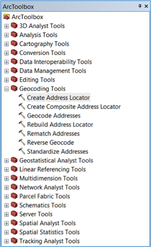
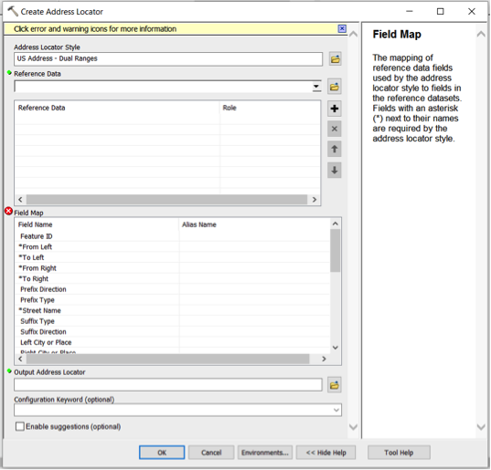
To create an address locator, use the “Create Address Locator” tool in ArcToolbox (see Figure 3.1).
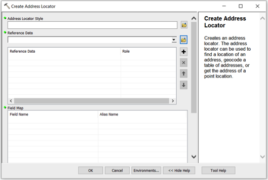
When you launch the tool, you are presented with the Address Locator dialog (see Figure 3.2).
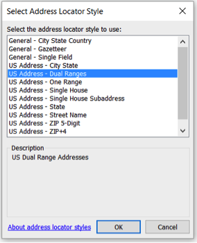
The first step in creating an address locator is selecting a locator style. The locator style which is most appropriate depends on the reference data you’re planning to use in addition to the format of the locations you’re trying to geocode. A commonly used address locator style is the U.S. Addresses – Dual Ranges (see Figure 3.3).
Once the locator style has been selected, the Field Map list in the bottom portion of the Address Locator dialog is automatically populated (see Figure 3.4). Fields with an asterisk are required by the locator style, and fields without an asterisk are optional. Once you have loaded a reference dataset, you can map these fields to the corresponding fields in the reference data.
The second step in creating an address locator is defining the reference dataset or datasets which will be used. As mentioned above, there are many reference data sources which can be used. For example, you can use a linear feature class based on roadway centerlines such as the “Address Range-Feature Shapefile” TIGER/Line shapefiles we reviewed in Lesson 2. Alternatively, you could use a polygon feature class based on parcel boundaries or zip code boundaries. Yet another option would be to use a point feature class based on address points.
Once you have selected the reference data, you can map the fields associated with the address locator style you have selected with the corresponding fields in the reference data (see Figure 3.5).
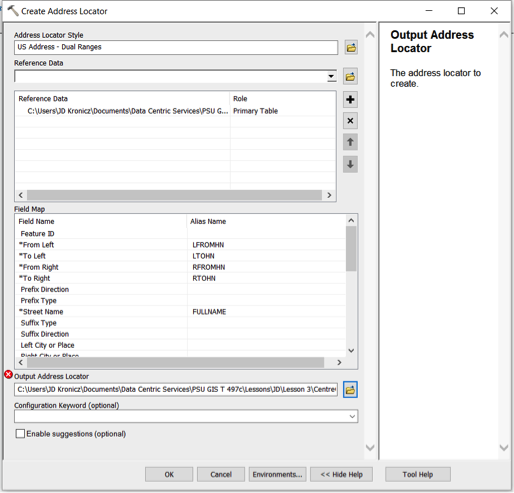
The final step is to save the address locator to a location you select. While you can store the locator in either a geodatabase or a file folder, ESRI recommends storing an address locator in a file folder for better performance.
Here is a link to an ESRI webpage where you can download a white paper [42] which tells you everything you’d ever want to know about address locators in ArcGIS.
Geocoding a List of Addresses (or other location descriptions)
To geocode a list of addresses, you should first add the table of addresses data to your map document in ArcGIS. The addresses to be geocoded can be prepared in any number of file formats including xlsx, xls, dbf, csv, and txt. Once the table of addresses has been added, you can right-click on the newly added table and select “Geocode Addresses” from the resulting context menu. At this point, you’ll be asked to select an address locator (see Figure 3.6).
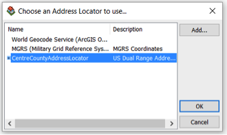
If the address locator you wish to use is not in the list, you can add it. Once you select an address locator and click “ok,” you will be presented with the “Geocode Addresses” dialog (see Figure 3.7).
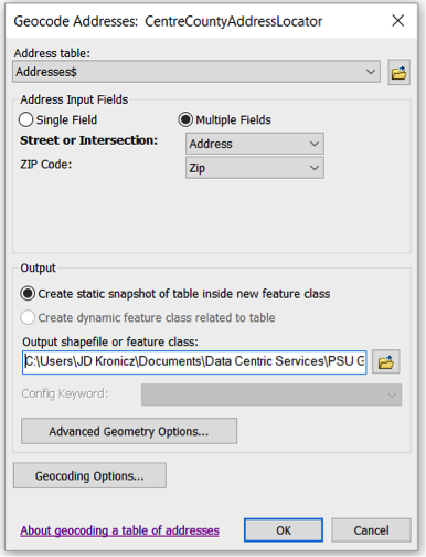
In the top portion of the dialog, you can map the fields in the input table to the corresponding fields in the address locator, if it isn’t done automatically, and define the location and name of the shapefile or feature class where the results of the geocoding process should be stored. You can also configure some parameters for the address locator by clicking the “Geocoding Options” button. The “Geocoding Options” dialog is then displayed (see Figure 3.8).
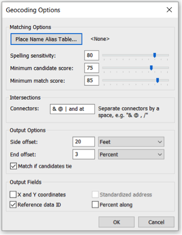
In the top portion of the dialog, you can exercise some control over how matching is performed. The spelling sensitivity level controls the extent to which misspellings will still be considered a match. The lower the score, the more tolerant the geocoding engine is for misspelled words. The minimum candidate score sets the threshold score for identifying candidates. The lower this score, the more candidates an address could have. Finally, the minimum match score establishes the threshold score for declaring a match for the address. Lowering the minimum match score will generally increase the match rate but will also tend to result in a higher rate of false positives.
The dialog can also be used to set other parameters for the geocoding engine such as offset positions for geocoded point features and some output data elements which can optionally be included as attributes in the resultant shapefile or feature class.
Once the geocoding options have been defined, the geocoding process can be initiated by clicking “Ok” on the “Geocode Addresses” dialog (see Figure 3.7). When the geocoding process is complete, a summary of the geocoding results is presented (see Figure 3.9).
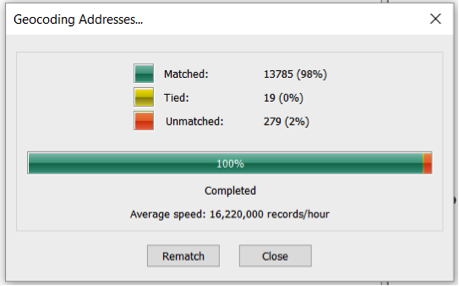
This summary shows the number of addresses which had candidates above the minimum match score (i.e., matches), the number of addresses which had multiple candidates which were above the minimum match score and had the same score (i.e., ties) and the number of addresses which did not produce any candidates above the minimum candidate score (i.e., unmatched).
From the results summary screen, a manual rematch process can be initiated by clicking the “Rematch” button. This brings up the “Interactive Rematch” screen (see Figure 3.10).
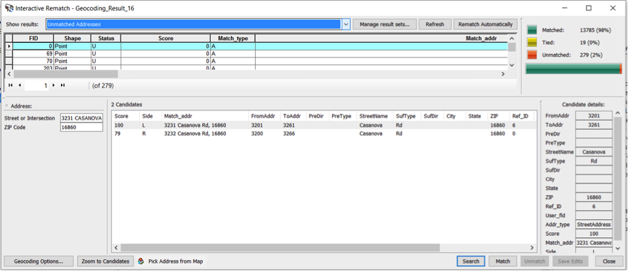
On this screen, unmatched addresses, ties, and matched addresses can be reviewed. Unmatched addresses generally result from either a problem with the address or a problem in the reference data. If a problem is observed with the address, it can be corrected and matched with the correct candidate directly on this screen. Often, however, it is unclear what the problem is with a particular address, and additional research is required to determine where the problem lies before it can be corrected.
3.2 Conflation
Conflation, in the context of GIS, is the process of combining two geospatial datasets so that the resultant dataset is superior to the input datasets. While conflation processes are used throughout GIS, they are of particular importance in GIS-T where roadway datasets of varying spatial quality and attribution are available from many different sources. The act of conflating datasets can often be a complex and time-consuming process. How complex and time-consuming the process is depends on a number of factors including the spatial extent of the datasets, the number of features present and the degree of spatial alignment between corresponding features. In some cases, it may be possible to automate a portion of the process but the success of these types of approaches depends on the quality of the initial datasets and the requirements for the final product.
Reference Dataset
When conflating two datasets, one of the datasets is generally considered to be the reference or target dataset. This is the dataset with the most spatially accurate features. The other dataset is sometimes referred to as the input or source dataset.
Conflation Workflow
While each conflation project can be unique, they all draw from a core set of activities. Some of the more common conflation activities include the following:
- Feature Matching: The objective here is to match corresponding features in the datasets. This process can be based on the spatial alignment of the features and/or certain attributes of the features.
- Feature Alignment: Once features are matched, they can be brought into spatial alignment with each other to establish proper topological relationships.
- Feature Addition: Features in the input dataset which are missing in the reference dataset can be added to the reference dataset.
- Attribute Transfer: Attributes information from the input dataset is added to the reference dataset.
The characteristics of the activities involved in a conflation project are largely dependent on the nature of the input datasets. There are three potentials scenarios:
- Vector - Vector
- Vector - Image/Raster
- Image/Raster - Image/Raster
In GIS-T, we are most commonly engaged in conflating two vector datasets (i.e., roadway data).
Horizontal Conflation vs. Vertical Conflation
Conflation can also be broadly categorized as horizontal conflation or vertical conflation based on the geographic relationship between the datasets. In horizontal conflation, the objective is to join two datasets which are spatially adjacent to each other. For example, perhaps you want to join roadway datasets from two adjacent counties or two adjacent states. In these cases, there is often some feature overlap near the dataset boundaries. In vertical conflation, the datasets being merged span the same geographic region or at least have substantial overlap. The objective is often to transfer a robust set of attribute data from one dataset, which may be of poor spatial accuracy, to a dataset which is poor in attribution but spatially accurate. Of course, in the real world, you may run across situations where the datasets partially overlap.
Conflation Tools
GIS software often has some built-in tools to at least assist with conflation needs. For example, in ArcMap 10.2.1, ESRI introduced a set of tools to help with conflation. The conflation toolset is found in the Editing Toolbox. ESRI also added a tool called Detect Feature Changes to the Data Comparison toolset in the Data Management Toolbox. Spend some time reviewing the help documentation for these tools.
3.3 Getting to Know a Transportation Organization
This week, we’ll take some time to explore Metropolitan Planning Organizations (MPOs) and Rural Planning Organizations (RPOs). MPOs were formed as part of 1962 Federal-Aid Highway Act and are required for any urbanized area with a population of more than 50,000. Congress recognized transportation planning is best done at a regional level since the nature of transportation systems and services often transcends an individual municipality, city, or county.
Watch the short video (11 minutes) below which discusses the purpose and structure of MPOs. There are more than 300 MPOs across the U.S., a listing of which is provided here [43].
Video: MPO Planning Process (11:27)
NARRATOR: Transportation is the backbone of our communities. We rely on it every day to get us to work, to get us to shopping and recreation, and to bring us goods and services. But who makes the decisions about our transportation system, and how are those decisions made? This video is an introduction to Metropolitan Transportation Planning and the role of metropolitan planning organizations.
Over the last 100 years or more, America's population and lines of commerce have expanded well beyond the boundaries of individual cities and towns. Today, networks of highways, transit services, freight carriers, and airports serve metropolitan areas that may include many cities, suburbs, towns, and counties. In today's urban areas, many transportation decisions are best handled at the regional level. A regional approach gives decision-makers a comprehensive understanding of transportation problems and the ability to develop comprehensive solutions.
Over the years, Congress has promoted a regional approach to urban transportation planning and decision-making. One of the most important advances came in the 1970s with legislation that required the creation of metropolitan planning organizations or MPOs in areas with a population of 50,000 or more. Now, there are over 300 MPOs across the country. An MPO may be a free-standing planning organization or an association of local governments, but every MPO is governed by a policy board of local elected officials. The Board may also include representatives from state transportation departments, mass transit operators, and others. The MPO is not alone in the decision-making process, but it's the engine that drives collaboration and cooperation among many participants. Local elected officials bring a unique perspective to the planning and decision-making process. They often face a challenging balancing act, making decisions that have the greatest regional benefit, while at the same time reflecting the concerns of the communities they represent.
MPOs and their partners produce three key documents: the Unified Planning Work Program, the Transportation Plan, and the Transportation Improvement Program. The Unified Planning Work Program (or UPWP) describes the planning studies that are being performed for the metropolitan area. The Transportation Plan identifies the region's transportation policies, strategies, and projects for the next twenty years or more. The Transportation Improvement Program (or TIP) is a short-range program of projects covering at least three years that directs available funds to those improvements that are the highest priority. The MPO Policy Board and its partners direct the development and content of the Plan, the TIP, and the UPWP. Both the Plan and the TIP must be fiscally constrained, in other words, consistent with available and expected funds. In areas with air quality problems, the Plan and the TIP must also help the region meet federal standards.
Let's now look at how the Plan and the TIP are prepared. Often the local planning participants start with a regional vision or a set of goals. This vision expresses what the region would like to become perhaps forty or fifty years in the future.
LES STERMAN: Well, important elements of a long-range plan are obviously a strong statement of goals and values, what is it that we're after, and transportation systems in the future.
NARRATOR: In developing a vision or goals, the MPO may consider many questions: What are the trends in regional growth, and are they desirable? How well is the transportation system performing? Do existing plans deal with current and expected problems? Can the transportation system support the kinds of future development that the region desires? When the vision and goals are in place, the MPO and its partners are better able to identify transportation problems and needs. These can include declining mobility, increasing congestion, poor access to jobs in neighborhoods, unhealthy air, or inconsistency with proposed economic development. An understanding of these problems allows the MPO and its partners to identify alternatives to improve transportation. Alternatives may include new policies, operational strategies, or capital projects. Some may help the existing system work better. Others may expand or build new transit lines, highways, and other facilities. Another round of questions is asked in assessing the impact of alternatives. How well does each alternative address the region's transportation problems? What are the likely impacts on neighborhoods and the environment? How much do the alternatives cost? Are the funds there, and is this the best use of available resources? The answers to these questions help the board choose the best alternatives. By adopting the Transportation Plan, the board establishes the policies, strategies, and projects that the region will pursue.
To develop the TIP, priority projects are drawn from the adopted Transportation Plan and matched with available funding. Once adopted by the MPO, the TIP is submitted to the state and becomes part of the statewide transportation improvement program, but the process doesn't end here. Projects and strategies in the plan and TIP undergo further development, often including engineering and environmental studies. Also, many MPOs monitor the implementation of the plan and TIP, study how well the plan is working, and make periodic adjustments. Federal rules require that the plan be updated and readopted every three to five years, and the TIP every two years.
RAE RUPP SRCH: Long-range planning, it is an ongoing process. It's not etched in stone, and many people don't realize that. New board members don't realize that either, that it's not a plan etched in stone. That, you know, it's constantly in an updating process.
NARRATOR: Agency and public involvement is a key activity in every step of the planning process. The public refers to a variety of individuals, agencies, and organizations each with different interests and levels of involvement. Many different approaches are used to inform and engage other agencies and the public.
CHARLES UKEGBU: Our public participation is not just at the MPO level, and that's one of the things we try to emphasize at the municipal level. It is not just the MPO calling a meeting, no, it is the MPO participating in other meetings and forums that may have been called by other, whether city or state agencies.
NARRATOR: Transportation planning continues to evolve. New issues are emerging that demand innovation and creativity from MPOs. Many MPOs today are working with other local and state agencies and the private sector to provide multi-modal systems that give people more choices. Transit, carpooling, bicycling, walking, better connections between highways, transit, airports, freight, and other modes of transportation can make the entire system work more efficiently.
DAVID PAMPU: We can't solve our transportation problem in key corridors just by widening the roads anymore. We have to provide some additional mobile opportunities for the traveling public. By focusing on rapid transit in conjunction with roadway improvements, we think we can add significant capacity for the traveling public.
NARRATOR: Coordinating transportation and land-use can be challenging. While transportation decisions are made at the state and regional levels, most land use decisions are made by local governments and private developers. The MPO may be the only place where officials from different jurisdictions can coordinate land use and transportation planning for the region as a whole. Many MPOs are partnering with state transportation departments, transit operators, and other agencies to preserve existing transportation assets and to squeeze more capacity out of their existing systems.
LES STERMAN: Probably for forty years, we chased congestion. Congestion was our number one goal, addressing congestion was our number one goal. But now we're recognizing that preserving existing system, our bridges and highways and our transit systems and the safety of that system are in fact more important goals, and we recognize them, and that's part of our vision. To create a system that's not only safe but is well maintained and preserved particularly in the core of our region.
NARRATOR: Planners are also making greater efforts to respond to the needs of all the users of transportation systems. People of every age, ethnic group, and income level because mobility is a link to opportunity and equality. For elected officials and citizens alike, Metropolitan Transportation Planning is a tremendous opportunity to build better communities.
JEFFREY SCHIELKE: I think I went into it not realizing, you know, that I was in a much wider, bigger area that had dramatic impacts until I got in the process and began to experience, you know, what other towns were going through and seeing and learning from their mistakes and learning their ideas. I think that's one of the rich rewards of the MPO process.
RAE RUPP SRCH: It's an exciting position to be in. You do have input, you're representing your communities. I think anybody that wants to get involved in this should.
JOHN MASON: It is basically a collaborative approach among the jurisdictions within a metropolitan region. There are some federal rules and laws that guide how we have to go through the process, but the real success of MPOs is based on the ability of the leaders of the jurisdictions to be able to collaborate to achieve a common goal.
Rural areas often have transportation needs that are very different from metropolitan areas. In rural regions, either the State DOT, a Rural Planning Organization (RPO), or a local government conducts transportation planning. While RPOs are not federally required, it is a requirement that if the state performs the planning function for rural regions, they need to coordinate with local officials.
In Pennsylvania, there are 15 MPOs and 8 RPOs. MPOs and RPOs often have strong GIS capabilities to support various planning studies.
3.4 Getting to Know Each Other
This week you’ll have a one-on-one chat with one of your classmates as per the schedule you were provided in Week 1. The discussion should be at least 30 minutes in length. If it’s the first time you’ve chatted with each other, spend the majority of time getting to know each other. Otherwise, focus on discussing the lesson content.
3.5 Webinar for Next Week
Speaker
Next week, our speaker will be Mr. Glenn McNichol. Glenn is a Senior GIS Specialist with the Delaware Valley Regional Planning Commission (DVRPC). He has been with the Commission for 23 years. As a member of DVRPC’s GIS unit, he supports the activities of the Commission’s planning staff through map production, data development, and GIS analysis. He also manages the Commission’s orthoimagery program.
Glenn holds a BA in Geography from Montclair State University. He also received a Professional Certificate in Geomatics from Cook College, Rutgers University.
The August 2016 edition of DVRPC News [45] featured a profile of Glenn (note: scroll to the bottom of the page to see the profile).
The Delaware Valley Regional Planning Commission (DVRPC)
DVRPC is a Municipal Planning Organization (MPO) responsible for 9 counties in the Philadelphia area, 6 of which are in Pennsylvania and 3 of which are in New Jersey.
DVRPC's stated vision and mission statements are shown below:
DVRPC’s vision for the Greater Philadelphia Region is a prosperous, innovative, equitable, resilient, and sustainable region that increases mobility choices by investing in a safe and modern transportation system; that protects and preserves our natural resources while creating healthy communities, and that fosters greater opportunities for all.
DVRPC’s mission is to achieve this vision by convening the widest array of partners to inform and facilitate data-driven decision-making. We are engaged across the region, and strive to be leaders and innovators, exploring new ideas and creating best practices.
DVRPC is engaged in many transportation projects [46]. Spend some time looking through a few of them.
3.6 Summary of Lesson 3
In this lesson, we discussed a number of geocoding techniques and considered the pros and cons of each. We also examined the properties of an address locator in ArcGIS and the role it plays in the geocoding process. You had the opportunity to construct your own address locator using TIGER/Line shapefiles and used it to geocode a series of addresses.
We also learned a bit about conflation especially in regards to roadway datasets. You then explored some of the tools in ArcGIS which can be used to conflate multiple datasets.
Our transportation organizations of the week were MPOs and RPOs. We learned about how they are structured and the responsibilities they have in the area of transportation planning.
In our weekly webinar, we had the opportunity to interact with Dr. Ira Beckerman, an archaeologist who leads PennDOT’s cultural resources group which is responsible for the Department’s compliance with Section 106 of the National Historic Preservation Act. We also had the opportunity to hear from Glenn McNichol, a Senior GIS Specialist with the Delaware Valley Regional Planning Commission (DVRPC).
In preparation for next week’s webinar, we took a look at DVRPC, a large MPO which handles the Philadelphia area, and explored the types of transportation projects they conduct.
Finally, you had the opportunity to get to know one of your classmates a little better and share some of your ideas and questions about this week’s lesson materials.
Questions and Comments
If there is anything in the Lesson 3 materials about which you would like to ask a question or provide a comment, submit a posting to the Lesson 3 Questions and Comments discussion. Also, review others’ postings to this discussion and respond if you have something to offer or if you are able to help.
Lesson 4: Transportation Networks
Learning Outcomes
What will we learn?
By the end of Lesson 4, you should be able to:
- describe the importance of a transportation network;
- characterize the data elements which go into a street network and evaluate street data sources to determine their suitability in serving as the basis of a network dataset;
- create a network dataset from street data;
- list the key functions of the Federal Highways Administration (FHWA);
- describe the composition and purpose of the National Highway System (NHS);
- discuss FHWA’s Geospatial Data Collaboration (GDC) initiative; and
- talk about the importance of addressing environmental and community considerations early in the transportation planning process and provide some examples of how GIS can be used to facilitate this process.
4.1 Transportation Networks
People and goods can move from one location to another by traversing a transportation network. There are many types of transportation networks including street networks, railroad networks, pedestrian walkway networks, river networks, utility networks, and pipeline networks. A geospatial model of a transportation network is comprised of linear features and the points of intersection between them. The modeling and analysis of networks has so many applications that there is an entire branch of mathematics devoted to it known as graph theory. In graph theory, linear segments of the network (e.g., road segments) are referred to as edges, and the points where the linear segments connect are called nodes.
Some transportation networks permit travel in both directions such as street networks and are referred to as undirected networks. Other networks generally limit travel to a single direction such as pipeline networks. These networks are referred to as directed networks. In ArcGIS, undirected networks are modeled with network datasets whereas directed networks are modeled as geometric networks. In this course, we will limit our study to street networks and the use of network datasets to model them.
Many transportation problems can be addressed through a network. A few examples are listed below:
- identifying the fastest, shortest, or most scenic path between two points on the network;
- determining the most efficient way for a delivery vehicle to visit a series of stops (also known as the traveling salesman problem);
- defining the service area around a given location;
- identifying an optimal store location.
We will take a detailed look at some of the more common network analyses in the next lesson. In this lesson, we will focus on the components of a transportation network model and the mechanics of creating one.
While a high-quality set of roadway centerline data is certainly a prerequisite to modeling a transportation network, it is by no means sufficient. Other important elements of a network model include the following:
-
Topology
The topology of a street network refers to the spatial arrangement and connectivity of the roads which comprise the network. Understanding how the road features relate and connect is critical to determining which paths or routes through the network are possible. Elevation is an important consideration in establishing network topology. Physical connections between streets require not only that they cross in the x-y plane but also that they cross at the same elevation. The picture below shows a complex interchange where many roads cross, but there are limited points of connectivity.
 Figure 4.1: Complex Highway InterchangeCredit: ESRI 2010 User Conference Technical Workshop
 -
Cost Attributes
In order to select the “best” route between two points in a network, you need to define what you are trying to accomplish. Perhaps you’re interested in determining the shortest route. In this case, you would need to know the distance between all adjacent nodes in the network. Consequently, the edges would need to have an attribute which quantifies length. Alternatively, if you want to know the fastest route between two points, you need to know the time it takes to move between any two adjacent nodes. Consequently, to support the fastest route determination, the edges need to have an associated time attribute or a speed limit attribute, since time is a function of length and speed limit. Regardless of how you define “best,” you need to have a corresponding attribute or attributes which allow the cost of potential routes to be quantified and compared. For example, if you want to know the most scenic route between any two points in the network, you would need to have a scenic score attribute associated with each edge which quantifies its scenic value.
-
Turns
Turns also play a key role in modeling a street network. One fundamental consideration in regards to turns is whether they are permitted. Many road intersections do not permit U-turns, for example. A second consideration for turns is the length of time they take. Left turns generally take longer to complete than right turns, since you generally have to contend with oncoming traffic. In order to accurately estimate how long it would take to traverse a network along a specific route, turn delays need to be taken into account.
-
One-Way Restrictions
Another important data element for a street network relates to one-way roads. In order to ensure that only legitimate routes are considered, roads which limit travel to one direction need to be identified.
-
Traffic
We all know that traffic plays an important role in determining how long it takes to traverse a particular route. Consequently, historic traffic data, or better yet, live traffic data, can be extremely useful in a street network model.
-
Directions
Often one of the desired outputs of network analysis is a set of description directions. In order to support the production of meaningful directions, a variety of descriptive roadway attributes needs to be present. Signpost data can also provide a valuable source of information for the creation of meaningful directions.
As you can see, a lot of information is required beyond basic roadway centerline geometry in order to create a street network which can support network analysis and produce high-quality results.
4.2 Getting to Know a Transportation Organization
This week, you’ll take some time to get to know the Federal Highways Administration (FHWA), an important agency within the USDOT. The roots of the FHWA trace back to its first predecessor organization known as the Office of Road Inquiry (ORI) which was created by President Grover Cleveland in 1893. In the days before the automobile, interstate travel was dominated by railroad and it was actually a bicycle boom which was largely behind the initial interest in improving America’s roads. An interesting history of the FHWA can be found here [47]. A signature achievement in the advancement of America’s roads was the development of the Interstate system of roadways championed by President Dwight D. Eisenhower. Today, the Interstate system represents about 50,000 miles of highway and is responsible for about one-quarter of the vehicle miles traveled on America’s roadways.
The primary function of the FHWA is to assist states and local governments with the design, construction, and maintenance of roads and bridges and to ensure US roads and highways meet a high standard of safety and quality. The primary mechanism through which the FHWA supports states and local governments is the Federal Aid Program. This program looks to focus federal monies on the nation’s most important roadways.
The Intermodal Surface Transportation Efficiency Act of 1991 introduced the concept of the National Highway System, a system of roads and highways deemed critical to America’s economy, defense, and/or mobility. Through the efforts of FHWA working with other federal, state, and local partners, roughly 160,000 miles of roadway were identified for inclusion in the NHS. The National Highway System Designation Act of 1995 signed into law by President Bill Clinton officially designated these roadways as the NHS.
A brief but informative article on the NHS titled The National Highway System: A Commitment to America's Future [48] appeared in a 1996 edition of Public Roads, a bimonthly magazine published by FHWA.
One of the FHWA’s key objectives is to encourage innovation and to provide states and local governments with needed technical assistance. A recent FHWA initiative known as Geospatial Data Collaboration [49] (GDC) is aimed at promoting the use of GIS tools to facilitate data sharing and increased collaboration between transportation agencies and resource agencies, with the ultimate objective of more timely project delivery.
4.3 Getting to Know Each Other
There are no one-on-ones scheduled for this week.
4.4 Webinar for Next Week
Next week we'll hear from 2 speakers.
Speaker #1
Our first speaker will be Mr. Frank DeSendi. Frank is the Manager of PennDOT’s Geographic Information Division and is also a former Chair of the American Association of State Highway Transportation Officials’ GIS for Transportation (AASHTO GIS-T) Task Force. He began his career with PennDOT in 1989 and has been working in the geospatial field since 1995. Frank holds a Bachelor of Science in Geography from The Pennsylvania State University.
One interesting use of spatial technology which Frank’s group implemented a few years ago is called LPN which stands for Linking Planning and NEPA. PennDOT and its planning partners (i.e., the MPOs and RPOs) use the application to screen potential projects against more than forty environmental datasets which collectively address most NEPA concerns. Based on the proximity of a proposed transportation project to these resources, the application determines a score which can be used to compare various alternatives for the project. The user’s guide for the application is here [50].
Planning and Environmental Linkages (PEL)
In the past, transportation planning and the development of TIPs and STIPs occurred with little thought given to environmental and cultural resources and community concerns. Later in the project development process, when the design and construction of the project were imminent, the potential impacts to these resources were considered as is required by NEPA. If through this NEPA review process, the project was anticipated to have potential impacts on these resources, it often led to substantial delays in project delivery, unexpected increases in the project budget, and a less than ideal solution for all involved. Consequently, significant efforts have been made in the past 15 years to begin assessing potential impacts to resources early in the planning process and for transportation agencies to work more closely with resources agencies. Spatial technologies have played a large role in facilitating potential impact assessments, identifying alternatives that eliminate or minimize impacts and, when impacts are unavoidable, identifying mitigation strategies which can offset any negative impacts of the project.
In response to the need to more closely integrate transportation planning and environmental review, FHWA created the Planning and Environmental Linkages (PEL) program to help state DOTs, MPOs and RPOs revise their planning processes, improve their coordination with resource agencies and develop tools to streamline the entire process.
Watch the 2011 webinar (72 minutes) jointly sponsored by FHWA and AASHTO titled Linking Transportation and Natural Resource Planning through the use of Environmental GIS Tools [51].
Speaker #2
Our second speaker will be Mr. Greg Ulp. Greg is a Senior Project Manager with GeoDecisions, a division of Gannett Fleming specializing in GIS and IT. He has over 25 years of experience in applying spatial technologies to solve transportation problems and has worked with a number of state DOTs. Greg has worked extensively with the Pennsylvania Department of Transportation’s GIS Division. He was the technical architect for a GIS application called the Multimodal Project Management System Interactive Query (MPMS-IQ) which is used to access and visualize data for the Department’s highway and bridge projects. Greg holds a bachelor’s degree in computer science from The Pennsylvania State University.
Transportation Planning
There are a number of transportation plans that regional planning organizations (MPOs and RPOs) and state DOTs are federally required to prepare and periodically update. These include the following:
- Long Range Transportation Plan (LRTP)
An LRTP, also known as a Regional Transportation Plan (RTP), is a long-term plan which is prepared by an MPO. It typically has a 20 to 30-year horizon and is updated every 3 to 5 years. The LRTP establishes priorities and long-term objectives for the region. - Transportation Improvement Program (TIP)
The TIP is a short-term plan, at least 4 years in length, which aligns with the policies and objectives defined in the LRTP. Each MPO is federally mandated (49 U.S.C. 5303(j)) to develop a TIP which includes all federally funded projects in addition to non-federally funded projects which are consistent with the LRTP. The TIP is required to be in line with available funding (i.e., fiscally constrained). - Statewide Transportation Improvement Program (STIP)
The STIP is a statewide roll-up of each of the TIPs across the state and is maintained and updated by the state DOT. The STIP is also federally mandated (23 U.S. Code § 135). Each state’s STIP is subject to approval by both the Federal Highways Administration (FHWA) and the Federal Transit Administration (FTA) (two organizations we’ll take a look at in upcoming lessons).
Project Visualization Tools
In order to solicit feedback from the public on potential projects and to provide legislators and the public access to information on planned and active projects, state DOTs, Municipal Planning Organizations (MPOs) and Rural Planning Organizations (RPOs) sometimes use web-based GIS applications to enable people to visualize projects in a specific geographic area and get detailed information on a project of interest.
Watch this FHWA sponsored webcast on Visualizing TIPs and STIPs Using GIS [52] which was held on April 27, 2016. It is a little rough in spots but is very informative. The presentation doesn’t actually start until about 7 ½ minutes in, due to some technical difficulties. In the webcast, PennDOT discusses three separate GIS-based project visualization applications which are used to provide the public and state legislators access to planned and active projects. All three applications have a consistent user interface and differ only in the types of projects they show. The first application shows active projects under construction, the second shows Act 89 projects which are projects of particular interest to state legislators and the third shows planned projects (i.e., projects on the STIP and TYP). All three applications can be accessed here [53].
Another organization which participated in the webcast was the Delaware Valley Planning Commission (DVRPC). DVRPC is an MPO which spans 9 counties in 3 states (Pennsylvania, New Jersey, and Delaware). In the webcast, DVRPC discusses how they make project information available through a Google Maps-based GIS application. Take some time to explore the 2017 DVPC TIP Visualization tool [54]. In addition to using GIS to facilitate visualization of their transportation program, DVRPC also uses spatial technologies to evaluate potential projects for the TIP based on a variety of criteria they have developed.
MPMS-IQ
MPMS-IQ is a web-based GIS application developed for PennDOT which allows users to visualize projects and access a wide variety of project related information via a map interface. The projects which are available through MPMS-IQ include active construction projects in addition to projects on PennDOT’s Twelve Year Plan (TYP). Unlike the STIP, the TYP is not federally mandated. The STIP corresponds to the first 4 years of the TYP. Take some time to explore MPMS-IQ [55]. In particular, look at the methods by which users can search for projects, the information available for each project, and the additional layers and features the application provides.
Additional Learning
TELUS is a research and innovation program funded through a grant from the FHWA designed to create spatially-enabled tools to assist MPOs and state DOTs in preparing TIPs and performing other transportation planning functions. TELUS software is created and maintained by the New Jersey Institute of Technology (NJIT). Information about the tools, including demos and download links, can be found here. [56]
4.5 Summary of Lesson 4
In this lesson, we learned about transportation networks. Specifically, we examined the elements which comprise a network and the activities that go into creating one. You then had the opportunity to solidify this knowledge by modeling a transportation network in ArcGIS through the construction of a network dataset from roadway centerlines and other associated data.
Our transportation organization of the week was the FHWA. You learned a little about the history and key roles of the FHWA. We also took a look at NHS, a network of roadways deemed critical to the nation, and FHWA’s geospatial data initiative known as the GDC.
We also had the opportunity to hear from two speakers this week. Glenn McNichol, a Senior GIS Specialist with the Delaware Valley Regional Planning Commission (DVRPC) and Michael Ratcliffe, the Assistant Division Chief for Geographic Standards, Criteria, Research, and Quality in the Census Bureau’s Geography Division.
In preparation for next week’s webinars, we learned how transportation planning and the NEPA review processes which seek to assess and mitigate environmental impacts related to transportation projects have become more tightly integrated and about the role GIS has played in helping to bring the two together. We also took a look at some GIS applications used to visualize planned and active transportation projects.
Questions and Comments
If there is anything in the Lesson 4 materials about which you would like to ask a question or provide a comment, submit a posting to the Lesson 4 Questions and Comments discussion. Also, review others’ postings to this discussion and respond if you have something to offer or if you are able to help.
Lesson 5: Network Analysis
Learning Outcomes
What will we learn?
By the end of Lesson 5, you should be able to:
- list the common types of problems that network analysis can be used to solve;
- use ESRI’s Network Analyst extension to perform a variety of network analyses;
- list some of the key functions state DOTs serve and discuss how their roles have changed over time;
- provide an example of how spatial technologies are used within a specific state DOT;
- discuss the nature of a Linear Referencing Systems (LRS) and dynamic segmentation and explain why these techniques are important in managing the geometry and diverse set of attribute information associated with transportation networks;
- share something you learned about one of your classmates and/or some ideas you discussed with a classmate about the content of this week’s lesson.
5.1 Network Analysis
Network analysis can be used to solve many different transportation problems that would be very challenging to solve otherwise. A prerequisite to performing network analysis is that you have a network model. In ESRI’s terms, this is a network dataset. We walked through an exercise to construct a network dataset in the last lesson. Of course, it is not a requirement of network analysis that you construct your own network model. There are a number of commercially available network models you can use instead.
The types of problems which network analysis can be used to solve are quite varied. One common characteristic of the algorithms that power each is that they involve determining the cost of one or more routes through the network. The cost is most commonly based on time or distance, but you can define a cost attribute any way you want. For example, you might score each edge in the network based on its scenic value. You could then create a cost parameter based on the scenic score and use the solver to find the most scenic route.
ESRI provides 6 out-of-the-box network analyses as a part of Network Analyst. ESRI terms these network analyses “solvers.” The solvers are listed below along with a brief description of each:
Route Solver
The route solver determines the best route between two or more points. Most of us use this network analysis on a regular basis. Whenever you use Google Maps or a comparable service to get directions from one location to another the service is conducting a network analysis to determine the best, typically fastest, route. This solver can route any number of points according to a specified order (i.e., the traveling salesman problem) or the most efficient order.
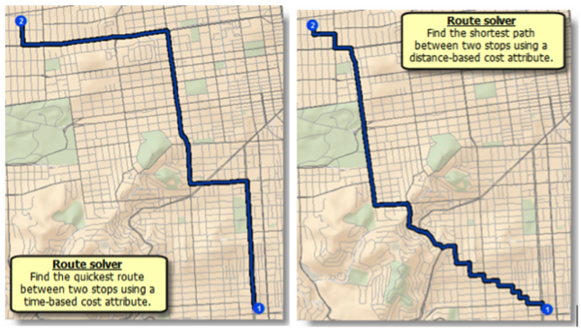
Closest Facility Solver
This solver is used to determine the closest facility to a given location. The term "facility" can be a bit misleading. For example, this solver could be used to determine the closest ambulance to an accident scene. In this case, using ESRI’s terminology, the ambulances would be considered facilities.
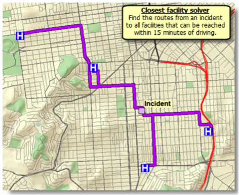
Service Area Solver
The geographic region which can reach a designated facility in a certain period of time (or vice versa) is termed a service area. To determine the bounds of this area, you can use the Service Area Solver.
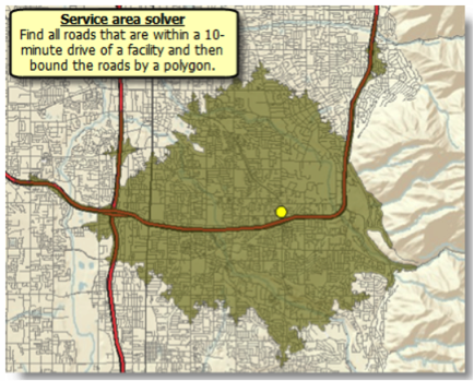
Origin-Destination (OD) Cost Matrix Solver
The OD cost matrix solver is generally used to determine the distances of the fastest routes between a set of origins and a set of destinations. Although the path between each origin and destination is often represented as a straight line, the route which corresponds to the time and distance costs between each pair of locations follows the street network.
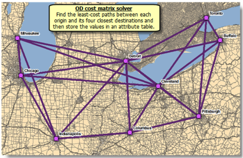
Vehicle Routing Solver
The vehicle routing solver is typically used to determine the most efficient routes for a fleet of vehicles tasked with servicing a series of stops.
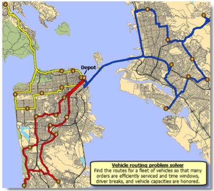
Location-Allocation Solver
The location-allocation solver can be used to determine how effectively a facility site is servicing locations which have a need for its services. As such, it can be used to select the best location for a facility from a series of candidate locations.
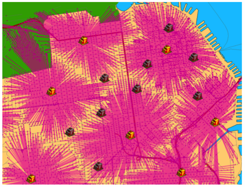
5.2 Getting to Know a Transportation Organization
This week, we’ll take some time to explore state Departments of Transportation (DOTs). All 50 states have a department of transportation, and while there are many similarities between them, they can differ in both how they are organized and in the specific functions they perform. A convenient set of links for all 50 state DOTs [58] is maintained by FHWA.
The origins of most state DOTs trace back to the early 1900s. At that time, they were commonly named State Highway Departments and, as the name implies, their focus was almost exclusively on highways. In the 100 or so years since then, their roles have evolved, and the responsibilities have increased dramatically. Today, state DOTs typically operate or oversee all modes of transportation within the state, and the scope of their functional responsibilities have grown from engineering and construction to include planning, safety, assessment, and mitigation of project impacts on the environment and community resources, driver’s licensing and vehicle registration, permitting, and providing technical support and oversight for local roads. A good summary of the roles and responsibilities of a state DOT is provided in Chapter 2 [59] of the National Cooperative Highway Research Program’s (NCHRP) Report No. 750 titled “Strategic Issues Facing Transportation, Volume 5: Preparing State Transportation Agencies for an Uncertain Energy Future [60] (2014).”
Given the extensive number of functions a state DOT is responsible for performing, there are a tremendous number of opportunities for applying spatial technologies, some of which we have looked at already (FHWA maintains a searchable compilation of state GIS-T projects [61]). Consequently, state DOTs have a substantial need for GIS expertise, although the degree to which these needs are outsourced varies. GIS expertise within the DOT is often housed in their planning or information technology organizations. AASHTO maintains a list of GIS-T contacts [62] for each state.
5.3 Getting to Know Each Other
There are no one-on-ones scheduled for this week.
5.4 Webinar for Next Week
Next week, we'll hear from 2 speakers.
Speaker #1
Our first speaker will be Mr. Bill Schuman. Bill is the Sr. Vice President of Project Delivery for Transcend Spatial Solutions. His responsibilities include project manager oversight; providing subject matter expertise for road inventory, asset management, linear referencing systems (LRS), and road data models; business operations; and guiding the company’s strategic direction. He has over 28 years of transportation and GIS experience. He is a recognized LRS and transportation data expert and has worked with state and local governments on IT strategic plans, spatially enabled database and data warehousing projects, LRS design and implementation projects, and many custom data maintenance and data presentation applications.
Bill holds a B.S. in Civil Engineering from the University of Wyoming and is a GIS Professional.
Linear Referencing Systems (LRSs)
Transportation agencies capture a wide variety of information about their roadways in addition to information about assets or occurrences along their roadways. Some of these attributes relate to a specific location (e.g., crashes) while other attributes relate to a section of roadway (e.g., speed limit). Collectively, these point or linear attributes are referred to as events.
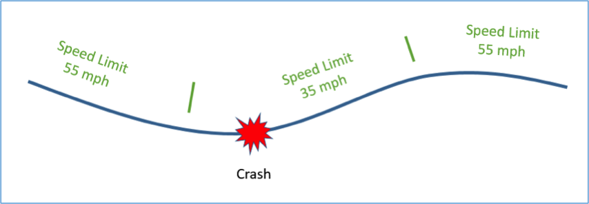
The large number of events which need to be associated with the geometry of the roadway creates a challenge due to the fact that they often change values at different locations. For example, the locations where speed limit changes occur generally doesn’t correspond to the points where changes in pavement type, the number of lanes, or the condition of the roadway occur.
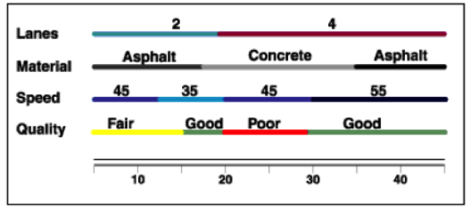
Consequently, if we were to attempt to segment the roadway in such a way to ensure all attributes were constant over the length of each segment, we would wind up with a highly segmented roadway. Alternatively, if we were to create a separate linear feature class for each roadway attribute, we would have a large number of feature classes that would need to be maintained. One solution to this problem is to separate the events data from the route geometry and maintain them in separate tables which relate to the route geometry according to the route name and a linear measure (for point events) or pair of measures (for linear events) which indicate the location of the event along the route.
There are many different ways one can locate an event along a route. For example, an event could be located according to its distance along the route in miles from the county line. Alternatively, the distance could be measured from the beginning of the route or some other established marker or datum. These different approaches are referred to as Linear Referencing Methods (LRMs).
Given the relationship between the events in the events table and the route features, GIS software can dynamically create feature classes for any specific event or combination of events. This process is known as dynamic segmentation. The standard set of geoprocessing tools can then be applied to these dynamically generated features just as they can be applied to a persistent feature class.
The entire system which an organization uses to allow for the separation of event data and dynamic generation of feature classes is known as a Linear Referencing System (LRS). LRSs have been used extensively with road networks, but they are applicable to other types of linear networks as well, including pipelines and hydrologic networks.
Speaker #2
Our second speaker will be Mr. Derald Dudley. Derald is a geographer and computer scientist in the Office of Spatial Analysis and Visualization (OSAV) which is part of the USDOT's Bureau of Transportation Statistics (BTS). He also chairs the Federal Geographic Data Committee (FGDC) Transportation Subcommittee.
BTS and the National Transportation Atlas Database (NTAD)
In April 1994, then-President Bill Clinton signed Executive Order 12906 titled “Coordinating Geographic Data Acquisition and Access: The National Spatial Data Infrastructure.” Since then, the FGDC together with their partner organizations have developed and revised a strategic plan to advance the National Spatial Data Infrastructure (NSDI). The most current version of the plan can be found here. [64] The USDOT’s Bureau of Transportation Statistics (BTS) [65] is responsible for overseeing the transportation components of the NSDI through the National Transportation Atlas Database (NTAD) [66]. Take some time to familiarize yourself with BTS and the NTAD. Also, take a look at the following datasets included in the NTAD: Highway Performance Monitoring System (HPMS) and the National Highway Planning Network (NHPN). Finally, read about the National Transit Map [67] which also generates datasets included in the NTAD.
5.5 Summary of Lesson 5
In this lesson, we learned about network analysis and the broad set of transportation problems it can be used to address. We examined how network analysis is implemented in ESRI's Network Analyst extension to ArcMap and examined the 6 categories of network analysis or solvers which it provides. In addition, you had the chance to get some hands-on experience with a few of the solvers. You will have additional opportunities to apply these tools in upcoming lessons as well.
Our transportation organizations of the week were state DOTs. We reviewed some the key functions these organizations perform and looked at how their roles have changed over the past century. You also explored a state DOT of your choice and became familiar with an example of how they use spatial technologies.
In our weekly webinar, we had the chance to interact with Frank DeSendi, the Manager of PennDOT's Geographic Information Division, and review how PennDOT utilizes spatial technology to help them identify potential impacts a transportation project could have on the environment. We also had the opportunity to interact with Greg Ulp, a senior project manager who was the technical architect for MPMS-IQ, a GIS application used by PennDOT to disseminate project information to the public and other interested parties.
In preparation for next week's webinar, we learned a bit about LRSs and dynamic segmentation, important topics in GIS-T which we will cover in more detail in next week's lesson. We also learned about the National Transit Atlas Database (NTAD) and some of the important datasets it contains.
Questions and Comments
If there is anything in the Lesson 5 materials about which you would like to ask a question or provide a comment, submit a posting to the Lesson 5 Questions and Comments discussion. Also, review others' postings to this discussion and respond if you have something to offer or if you are able to help.
Lesson 6: Linear Referencing Systems (LRS)
Learning Outcomes
What will we learn?
By the end of Lesson 6, you should be able to:
- use ArcMap’s Linear Referencing Tools to construct routes from roadway centerline features;
- calibrate the measures along a route based on actual measures made in the field;
- describe the purpose and characteristics of a Straight Line Diagram (SLD);
- create an SLD given event data along a route;
- discuss the key functions of the American Association of State Highway and Transportation Officials (AASHTO);
- discuss some emerging technologies in Intelligent Transportation Systems (ITS) and the objectives and features of traveler information systems;
6.1 Linear Referencing Systems
Last week, we explored the purpose and components of an LRS. This week, you’ll have an opportunity to solidify your understanding by completing some hands-on exercises to create routes, calibrating linear measures along a route, and using dynamic segmentation to convert event tables into event features. You’ll also see how GIS software can be used to reduce the burden associated with the creation and management of an LRS and event data.
6.2 ESRI Roads and Highways
In the past few years, ESRI has been promoting their Roads and Highways product which is designed to provide a fuller featured set of tools for transportation organizations to manage their LRS and roadway event data. A 57-minute introduction to this tool [68] was provided at the 2013 ESRI users’ conference.
Straight Line Diagrams
Transportation organizations capture and maintain a large number of linearly referenced roadway events including:
- Intersections
- Bridges
- Rail Crossings Locations
- Legal Boundaries
- Accidents
- Signs
- Speed Limits
- Average Annual Daily Traffic (AADT)
- Width of the Right of Way
- Width of the Roadway Shoulders
- Functional Class
- Curves
- Grades
- Projects
Displaying more than a few of these on a single map can begin to clutter the map and make it difficult for the user to understand.
One tool which transportation organizations have used for many years to visualize road attribute information is a Straight Line Diagram (SLD). In an SLD, a roadway section of interest is presented as a straight line along with various roadway attributes or events. Often, these roadway attributes are maintained by separate groups within the transportation organization, and sometimes they are linearly referenced using different LRMs. An SLD brings many attributes together with a uniform referencing method to facilitate visualization of the data and the potential identification of relationships between different data elements.
The specific layout of SLDs varies from one organization to another. One common layout for an SLD includes three components: a map component, a schematic component, and an attribute component. The map component often appears at the top of the SLD and presents the alignment of the route of interest. The schematic component, sometimes referred to as a stick diagram, presents the route as a straight line and can incorporate roadway features such as intersections, bridges, ramp entrances, and exits and legal boundaries. The attribute component includes roadway event data presented along the same horizontal axis. Linear events such as speed limit are displayed as a series of horizontal bars with the extent of each bar corresponding to the region over which the attribute has a constant value. Point events are displayed as point symbols positioned according to their location along the route.
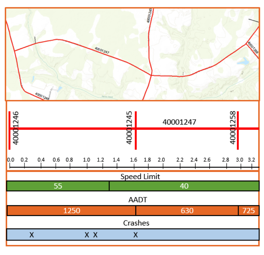
Historically, SLDs were manually created and assembled into books for reference across the organization. Given the effort required to generate SLDs in this manner, the books often reflected data which was somewhat dated. Today, most SLDs are created dynamically from current event data using sophisticated GIS software applications.
As an example, the Massachusetts Department of Transportation uses a web-based tool called Massachusetts Route Log [69] to generate Straight Line Diagrams (SLDs). Here is an example SLD generated from this application for a portion of State Route 9.
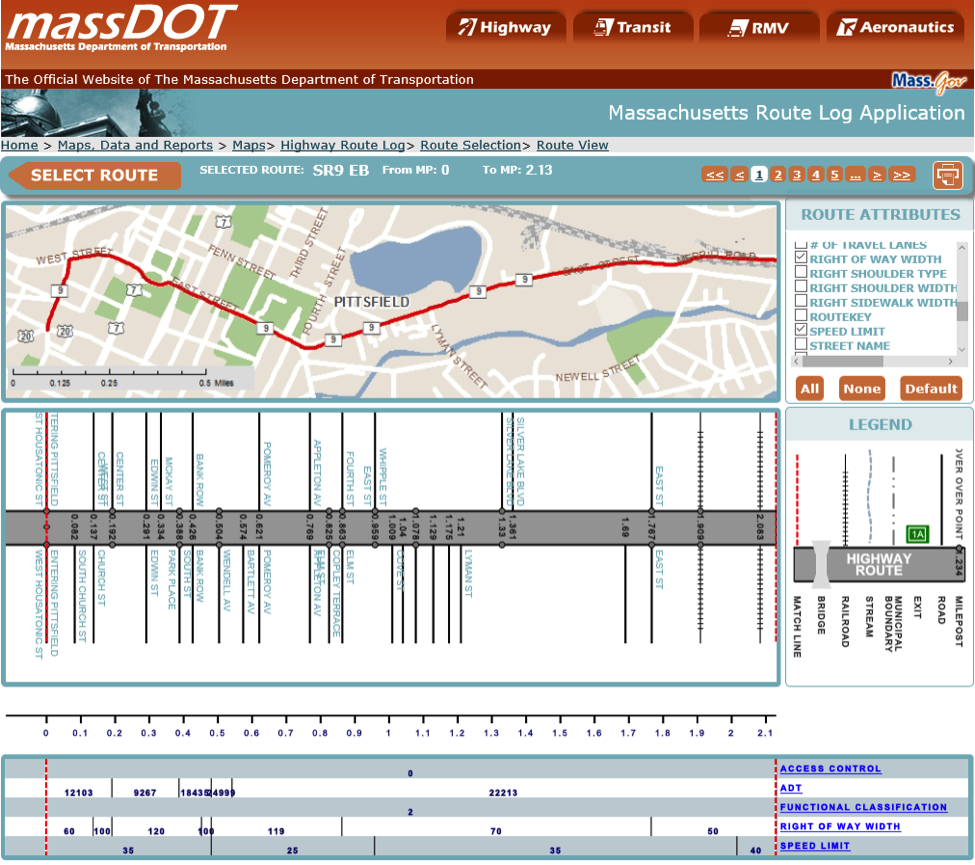
Vermont’s Agency of Transportation (VTrans) has a similar SLD tool called VTrans Routelogs [70].
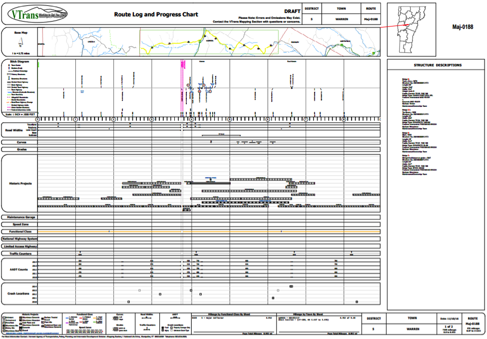
6.3 Getting to Know a Transportation Organization
This week, you’ll take some time to get to know the American Association of State Highway and Transportation Officials (AASHTO). AASHTO is an association comprised of representatives from the state transportation agencies in all 50 states, the District of Columbia, and Puerto Rico. AASHTO seeks to promote transportation excellence and integration across the U.S. and to foster effective communication and cooperation between the state DOTs and the federal government. Founded over a century ago, it was originally named the American Association of State Highway Officials (AASHO). As with state DOTs, its focus has broadened over the years, and in 1973, it was renamed the American Association of State Highway and Transportation Officials (AASHTO) to reflect the fact that its scope of activities spans all modes of transportation.
AASHTO administers a variety of technical programs. A few of their more significant areas of activity are briefly discussed below.
Standards and Publications
AASHTO establishes technical standards and guidelines which are generally adhered to by the state DOTs in addition to many organizations outside the U.S. It has published many highly respected and widely used reference documents spanning a variety of transportation disciplines including the following:
- A Policy on Geometric Design of Highways and Streets (also known as “The Green Book”)
- The Highway Safety Manual (HSM)
- Standard Specifications for Transportation Materials and Methods of Sampling and Testing
- AASHTO LRFD Bridge Design Specifications.
- Manual for Assessing Safety Hardware (MASH)
AASHTOWare
AASHTO manages a program aimed at providing exceptional enterprise level software to transportation agencies. These products incorporate the experience and expertise of its member organizations and have been developed using pooled funds from state DOTs and the FHWA. The suite of software developed in this program is collectively known as AASHTOWare and its products span 5 core business areas:
- Project
- Bridge
- Safety
- Pavement
- Right of Way
An overview of the AASHTOWare program is provided in this 7-minute video [71]. AASHTO also publishes a catalog of AASHTOWare products [72]. Many of the AASHTOWare software products incorporate varying levels of spatial technology. For example, the bridge products use the Google Maps API for spatial analysis and visualization.
Research
AASHTO is very active in the area of transportation research. A substantial portion of the research AASHTO promotes is carried out by the National Cooperative Highway Research Program (NCHRP).
AASHTO Materials Reference Laboratory
The AASHTO Materials Reference Laboratory [73] (AMRL) develops protocols for testing construction materials and accredits laboratories who test these materials. Many state DOTs require laboratories to be AMRL accredited before they will do business with them.
Centers of Excellence
AASHTO also operates the following three centers of excellence, each of which is designed to provide information and expertise in a specific area of transportation:
- Center for Environmental Excellence
This center focuses on environmental considerations associated with transportation. - National Operations Center of Excellence (NOCoE)
This center focusing on topics relevant to transportation operations. - Build America Transportation Investment Center (BATIC) Institute
This center focuses on funding and financing transportation projects.
6.4 Getting to Know Each Other
There are no one-on-ones scheduled for this week.
6.5 Webinar for Next Week
Speaker
Next week, we will have a webinar with Doug Tomlinson, Chief of Traffic Operations at the Pennsylvania Department of Transportation. Doug's career has focused on various aspects of traffic engineering including work zone traffic control, traffic signals, traffic calming, incident management, ITS, and Traffic Operations. He is currently a Chief of Traffic Operations for PennDOT's Bureau of Maintenance and Operations with a focus on Planning and Operations.
Doug has worked for PennDOT since 1994. He was named ITS PA person of the year by the Pennsylvania chapter in 2013. Doug was a graduate of PennDOT's first Executive Development Academy, as well as a 2008 Graduate of the Operations Academy. Doug graduated Magna Cum Laude from the University of Pittsburgh at Johnstown in 1993 with a B.S. in Civil Engineering Technology.
Intelligent Transportation Systems
Intelligent Transportation Systems (ITS) is an exciting subfield of transportation which encompasses a broad array of technologies. The unifying goals of ITS technologies and systems are to help us use our transportation network more effectively and to allow us to make more informed decisions. One of the most active areas within ITS is in the area of Connected Vehicles and Autonomous Vehicles (CV/AV). Check out this TED talk [74] (4:06) from 2011 on Google's driverless car:
Sebastian Thrun: Google's Driverless Cars (3:59)
As a boy, I loved cars. When I turned 18, I lost my best friend to a car accident. Like this. And then I decided I'd dedicate my life to saving one million people every year. Now I haven't succeeded, so this is just a progress report, but I'm here to tell you a little bit about self-driving cars.
I saw the concept first in the DARPA Grand Challenges where the U.S. government issued a prize to build a self-driving car that could navigate a desert. And even though a hundred teams were there, these cars went nowhere. So we decided at Stanford to build a different self-driving car. We built the hardware and the software. We made it learn from us, and we set it free in the desert. And the unimaginable happened: it became the first car to ever return from a DARPA Grand Challenge, winning Stanford 2 million dollars. Yet I still hadn't saved a single life.
Since, our work has focused on building driving cars that can drive anywhere by themselves -- any street in California. We've driven 140,000 miles. Our cars have sensors by which they magically can see everything around them and make decisions about every aspect of driving. It's the perfect driving mechanism. We've driven in cities, like in San Francisco here. We've driven from San Francisco to Los Angeles on Highway 1.
We've encountered joggers, busy highways, toll booths, and this is without a person in the loop; the car just drives itself. In fact, while we drove 140,000 miles, people didn't even notice. Mountain roads, day and night, and even crooked Lombard Street in San Francisco. (Laughter) Sometimes our cars get so crazy, they even do little stunts.
(Video) Man: Oh, my God. What? Second Man: It's driving itself.
Sebastian Thrun: Now I can't get my friend Harold back to life, but I can do something for all the people who died. Do you know that driving accidents are the number one cause of death for young people? And do you realize that almost all of those are due to human error and not machine error, and can therefore be prevented by machines?
Do you realize that we could change the capacity of highways by a factor of two or three if we didn't rely on human precision on staying in the lane -- improve body position and therefore drive a little bit closer together on a little bit narrower lanes, and do away with all traffic jams on highways? Do you realize that you, TED users, spend an average of 52 minutes per day in traffic, wasting your time on your daily commute? You could regain this time. This is four billion hours wasted in this country alone. And it's 2.4 billion gallons of gasoline wasted.
Now I think there's a vision here, a new technology, and I'm really looking forward to a time when generations after us look back at us and say how ridiculous it was that humans were driving cars.
Thank you.
Video: USDOT - Connected Vehicle: The Future of Transportation (7:29)
Imagine a future where vehicles talk to one another and to critical infrastructure. This connected vehicle technology can change our transportation system as we know it by enabling safe interoperable network wireless communications among vehicles, infrastructure, and personal communications devices. Connected vehicles provide drivers with 360-degree awareness of similarly equipped vehicles within a range of approximately 300 meters. This secure system keeps personal information private and does not track your vehicle. Drivers will receive warnings that inform them of potential hazards through a visual display, seat vibration, or tone. These are only warnings. The driver remains in control of the vehicle at all times. However, the technology can also support limited automated functions in which the driver only cedes partial control of the vehicle. Warnings can help drivers respond quickly to avoid potential crashes. For example, the intersection movement assist application warns drivers when it is unsafe to enter an intersection. The do not pass application warns drivers when it is not safe to pass a slower moving vehicle. The emergency electronic brake light application notifies the driver when an out-of-sight vehicle several cars ahead is braking, and imagine the value of this blind spot warning application which lets this commercial driver virtually see what's happening in his or her blind spot. Connected vehicles can communicate with smart roadside infrastructure like rail grade crossings to alert drivers when a train is coming even if the driver cannot see or hear the approaching train.
Connected vehicles can help with weather-related traffic and safety issues too. This is especially true with conditions such as black ice, where the weather may not appear to be dangerous, but the roads are slippery. Information collected from multiple connected vehicles can help determine when a potential hazard exists such as icy roads and warn drivers before they experienced them. Road weather data from the vehicles can be sent to traffic management centers or TMCs providing detailed, real-time information to help monitor and manage transportation system performance. The centers can then take actions like adjusting traffic signals and speed limits, notifying maintenance crews, dispatching maintenance vehicles to the road, and broadcasting warnings for motorists. Motorists can get real-time road weather information from in-car displays by dialing 511 or by listening to highway radio stations. Motorists will be able to get road weather information on their personal devices before leaving home.
Connected vehicles can even help us to reduce our carbon footprint and facilitate green transportation choices. Eco lanes are similar to today's HOV lanes, but with a big difference. Motorists in these lanes agree to drive eco-friendly vehicles and drive at a speed that conserves fuel. Drivers will be alerted about the proper speed with dynamic message signs.
Connected vehicle applications can help vehicles to reduce idling and unnecessary stops by communicating with smart traffic signals. Traffic signals broadcast data about their current signal phase and timing and systems inside the vehicles use the data to determine speed advice for drivers. Drivers could then adjust their vehicle's speed to pass the next traffic signal on green or slow down to a stop in the most eco-friendly manner, thereby saving fuel, reducing emissions, and saving drivers money. Connected vehicles can enhance awareness of unexpected roadside incidents like disabled vehicles, car crashes, police activity, and first responders caring for crash victims. Incident zone warnings will alert drivers about incidents ahead and warn them to slow down and change lanes. Communications could also be sent to first responders at the scene via shoulder radios to warn them of the danger of approaching vehicles. Connected vehicle technology can help control traffic flow and reduce the resulting congestion at accident sites before it gets out of hand.
With millions of connected vehicles, our ability to share robust data with each other and with smart infrastructure will continue to improve traffic flow, enhance coordination with transit, and make our communities even more safe and livable. The connection protection application gives public transportation providers and travelers the ability to communicate two ways. The connected network gives passengers real-time transit information so they can more accurately predict whether they will make their next connection. If multiple people on a delayed bus will miss their next connection, transportation providers can adjust bus departures to enable the passengers to make their next connection. Dynamic ridesharing applications make the logistics of ridesharing, scheduling, reliability, and communication easier by connecting vehicles and handheld devices. Applications do the matching for us, authenticating users and connecting riders with drivers. The co-operative adaptive cruise control app helps drivers avoid stops and starts, which can also help conserve fuel and improve traffic flow. And the queue warning app monitors traffic data to detect stretches of slow-moving traffic and warn motorists to reduce speeds to avoid potential rear-end collisions.
Connected vehicle technology can help pedestrians, too. For example, the mobile accessible pedestrian signal system app sends an automated pedestrian call from the smartphone of a pedestrian with disabilities to the traffic controller holding the walk signal until the pedestrian has cleared the crosswalk. This application also alerts drivers of the presence of a pedestrian with disabilities at the crosswalk.
The potential benefits of a connected transportation system, one that is able to enhance safety and mobility and address environmental impacts are wide-ranging. They will be felt by every one of us, enhancing the livability of our communities and ultimately making our transportation safer and smarter. Imagine the possibilities.
Traveler Information Systems
An area of ITS which has become very popular in recent years is traveler information systems. These systems disseminate real-time information to travelers in order to allow them to make more informed choices. These systems commonly contain the following types of information:
- Traffic and road conditions
- Construction projects
- Planned events
- Camera video and images
- Incidents
- Weather information
Traveler information can be disseminated by a number of methods including via Highway Advisory Radio stations (HAR), Variable Message Signs (DMS) and 511 websites, mobile applications, and IVR systems. On July 21, 2000, the Federal Communications Commission designated a single 3 digit number (511) which could be used anywhere in the nation to obtain traveler information. Implementation of the services themselves was left to states and local agencies.
The Federal Highways Administration (FHWA) hosts a 511 Travel Information Telephone Services [75] website which shows the locations in the U.S. which provide 511 telephone services. As you can see from this site, most states in the U.S. operate a 511 information service. If you click on any location with 511 telephone services, you'll be given more information about the 511 services of that state/location. You'll notice that there is a “backdoor” number you can use to call 511 in a state even if you are not in that state. The information provided also gives the link to the corresponding 511 website if there is one.
6.6 Summary of Lesson 6
In this lesson, we explored how GIS tools can be used to help maintain an LRS and event data. We also examined dynamic segmentation, a process used to convert event data into event features, and some very useful diagrams known as Straight Line Diagrams (SLDs).
Our transportation organization of the week was AASHTO. We reviewed some of the important roles AASHTO plays in establishing policy, producing important guidance documents, conducting and promoting research, and in creating exceptional software products for a number of functional areas in transportation.
In our weekly webinar, we had the chance to interact with Bill Schuman, Sr. Vice President of Project Delivery for Transcend Spatial Solutions, and benefit from his expertise and many years of experience in the area of LRS. We also had the opportunity to interact with Derald Dudley, a geographer and computer scientist with the USDOT's Bureau of Transportation Statistics (BTS).
In preparation for next week’s webinar, we also spent some time learning about intelligent transportation systems and, in particular, traveler information systems.
Questions and Comments
If there is anything in the Lesson 6 materials about which you would like to ask a question or provide a comment, submit a posting to the Lesson 6 Questions and Comments discussion. Also, review others’ postings to this discussion and respond if you have something to offer or if you are able to help.
Lesson 7: Highway Safety
Learning Outcomes
What will we learn?
By the end of Lesson 7, you should be able to:
- explain how traffic safety analysis is moving beyond traditional approaches which have focused solely on historic crash data;
- navigate the Fatality Analysis Reporting System (FARS) and perform ad-hoc queries of the data it contains;
- use crash data extracted from FARS or other state crash data systems to visualize and analyze the data in ArcGIS;
- list some of the uses and benefits spatial technologies offer in the area of highway safety;
- describe some of the goals and objectives of the National Highway Traffic Safety Administration (NHTSA);
- submit a review of Pennsylvania's 511 Traveler Information System;
- discuss the purpose of the Highway Performance Monitoring System (HPMS) and the requirements it imposes on state DOTs;
- share something you learned about one of your classmates and/or some ideas you discussed with a classmate about the content of this week’s lesson.
7.1 Highway Safety
Highway safety is an important area of focus for state DOTs and the USDOT. There are few groups within the USDOT who are focused on improving highway safety. The first is the Office of Safety. The Office of Safety is comprised of two units. The Technologies Unit deals with safety-related highway design considerations and technologies which can be used to improve highway safety performance. The Programs Unit oversees federal and state safety programs. One of the key programs they administer is the Highway Safety Improvement Programs (HSIP). HSIP is a federal-aid program designed to provide funding to states for projects aimed at reducing fatalities and serious injuries on qualifying roadways. In 2016, the program provided about 2.2 billion dollars to the states for safety projects.
| Fiscal Year | 2016 | 2017 | 2018 | 2019 | 2020 |
|---|---|---|---|---|---|
| Estimated Funding* | $2.226 B | $2.275 B | $2.318 B | $2.360 B | $2.407 B |
Reference: FHWA Website [76] accessed 12/31/2016
To qualify for HSIP funds, a state is required to develop and maintain a Strategic Highway Safety Plan (SHSP). An SHSP is designed to guide the investment of funds to projects which have the greatest potential to reduce fatalities and serious injuries. To qualify for HSIP funds, states are also required to identify their priorities using a Data-Driven Safety Analysis (DDSA).
The second group within USDOT which is responsible for highway safety is the National Highway Traffic Safety Administration (NHTSA). NHTSA is an administration within USDOT whose mission is to reduce crash fatalities and injuries. We’ll take a close look at NHTSA later in this lesson.
State DOTs commonly collect and use crash data to identify areas of their roadway networks where there are unusually high crash rates. However, looking at crash data alone can be misleading and result in a less than optimal use of available state and federal dollars. To address this problem, AASHTO, in conjunction with the FHWA, developed the Highway Safety Manual (HSM), a document which many consider the definitive reference on highway safety. The HSM offers a comprehensive and balanced approach and set of tools which consider operations, the environment, and the cost of construction alongside safety considerations. A good overview of the HSM can be found here. [77] The approaches provided in the HSM go beyond traditional approaches to identifying priority locations for safety improvements which rely solely on crash history data.
There are two fundamental problems associated with using crash data alone. First, crashes are statistical events and as such don’t occur at regular predictable intervals. Consequently, crash data alone can sometimes lead an agency to falsely identify sections of a roadway as high risk and, conversely, sometimes overlook a risky section. The second problem of looking solely at historic crash data is that it disregards the dependence of crash frequency on traffic. As traffic levels increase on a section of the roadway due to changing travel patterns, crash rates can increase. To overcome these limitations, it is necessary to look not only at historic crash frequencies but also at expected crash frequencies based on roadway characteristics and traffic data.
Tools have been developed which implement the approaches defined in the HSM. These include AASSHTO’s Safety Analyst and FHWA’s Interactive Highway Safety Design Model (IHSDM). However, states often lack much of the data required to effectively use these tools, such as horizontal and vertical curve data. Horizontal curves are roadway curves that turn to the left or right, and vertical curves are roadway peaks/hills and valleys. For my Capstone Project, I used roadway centerline data to extract horizontal curvature data from Pennsylvania’s roadways. I gave a lightning talk on the project at Penn State in November 2016 for GIS day. My presentation was just under 10 minutes in length (embedded video below).
Host: JD are you ready?
Host: Alright! JD Kronicz will be our next speaker and he will talk about using GIS to identify and characterize horizontal curvature. JD has worked as a consultant for over 25 years serving clients in the scientific, environmental, transportation, and manufacturing industries. For the past 15 years, he’s been primarily focused on GIS software applications for transportation. He works closely with the Pennsylvania department of transportation and he also teaches in Penn States online geospatial program.
JD: Good afternoon. Today I have the pleasure of talking to you briefly about some work I did using GIS to identify the horizontal curvature in the roadways.
So, curves, as one might guess are an important feature of roadways when it comes to highway safety. Surprisingly, many state DOT’s, departments of transportation, don’t have good inventories of their roadway curves. Often if they have curvature information it’s embedded on engineering diagrams or other plans and really not in a format that is readily accessible for highway safety analysis. So, in this project I basically focused on trying to extract that information and producing an inventory of Pennsylvania’s horizontal curves from roadway centerline data which is data all state DOT’s have.
Now, it’s a priority of state DOTs to make sure that their roads are safe and to constantly try and improve safety. Generally, is what they’re trying to do is their trying to use the limited amount of safety dollars to apply to those roads that would best benefit, where they could make the biggest impact and get the biggest bang for the buck. The question is, how do they identify their priorities? And there’s really two different ways you can approach the problem.
The first, is by doing crash analysis. States all have good data on their crashes, and you can use the crash data to identify areas where there are high crashes and, in that manner, identify your priority sections of roadway. That’s a reactive approach and it may be erroneous because it could just be an anomaly, it might not represent a section of roadway that inherently has safety issues.
The other approach is to do a systemics analysis of the roadways where you’re looking at the characteristics of the roadways and your calculating the expected crash rates based on features of the road such as curvature features.
Either way once you identify the priority sections of roadway you want to improve safety on you can implement any one of many many counter measures or safety improvements. So here I’ve just shown a few and I could probably put together 100 but for example, center-line rumble strips, high friction surface treatments are just a couple.
Ok, so before I get into what approach I used, just a little bit on the geometry of the horizontal curve, this is kind of a complex figure but really all we’re interested in is 3 parameters when it comes to horizontal curves. We’re interested in the radius of the curve; we’re interested in the length of the curve and we’re interested in the central angle of the curve: the number of degrees in which the curve turns. So those are the 3 parameters we’re interested in and given any 2 of those parameters we can derive the 3rd.
So, the approach that I used was I started with roadway centerline data for Pennsylvania and I basically took each road feature and deconstructed into its ordered series of vertices which is basically what it represents and then for each pair of vertices I determined the straight line that went through those vertices and determined the baring angle, the angle between that straight line and the positive x-axis.
And then I continued to do that for each pair of ordered vertices in sequence. Basically, looking at how that baring angle changed and anytime the change in baring angle exceeded a certain threshold value I threw up a flag and said we’re in a curve. So that’s how we determined the start of the curve and continuing that process stepping through the vertices and when we get to the point where we drop below that threshold value, we know the curve ended. Any by aggregating the change in baring angle we can calculate the central angle of the curve; we can calculate the length and from those two we can derive the radius.
Again, if we had a little bit more time, we could get a little bit more detail on what the approach was but at the end of the day, by using this technique we can establish curve features that have attributes of radius, central angle, length, etc.
Now to do this sort of process manually would be extremely time consuming so I derived a, I created a program in python, implemented that as a custom toolbox in ArcGIS and named it curve detective. Essentially, it automates that algorithm I just kinda walked you through.
So, here’s an example of an output of that tool. You can see super imposed or layered on top of the roadway network we have this new curve feature class that this tool created. Each curve in red, labeled according to central angle and radius.
I then went ahead and processed, once I established it worked okay, I processed all the state roadway in Pennsylvania. So, in Pennsylvania, the state actually owns roughly 45 thousand miles of roadway. There’s a lot more roadway that’s local roads but the state actually owns and maintains about 45,000 miles of roadway. In order to process this roadway, it took the tool about 2 hours and it ultimately identified 170,000 or so horizontal curves.
Then I went ahead and I wanted to make sure that the output of the tool was legitimate, that it was accurate and precise so I went ahead and found locations that had been survey in the field and presumably had good data on the curves and then compared those engineering diagrams which is where that data is embedded to the results of the curve detective. Without getting into any great detail with you I found that the tool was very accurate and reasonably precise.
Ok, so at this point I had identified, or created an inventory of horizontal curves in Pennsylvania, and I wanted to basically see what could I learn by using the crash data we have in Pennsylvania and combining the two, just to see how crash rates differ on curves and I created a little tool on Microsoft access where I brought these two data sets together that allowed me to perform a bunch of analyses and I did conduct a number of analyses, I’ll just walk you through a couple briefly.
So in the first one I basically just looked at all the road sections in Pennsylvania that have a horizontal curve based on the output of the curve detective and I looked at the number of crashes, the crash rates on those sections of roadway and compared them to crash rates on straight sections of roadway and what I found is that one curves the crash rate is about 2.3x higher than on straight sections of roadway. I then went ahead and limited the crashes I was looking at just to crashes that involved fatalities. And when we just limit it to fatal crashes, we see that the crash rate is 2.8x times higher on the curved sections of roadway than it is on straight sections of roadway. So, not only are crashes more frequent on curves, they’re generally more serious.
I also looked at, I wanted to see the relationship between the central angle of the curve and the radius of the curve and the crash rate so I ran a series of analyses at various central angles, various radii and what I saw was there was little or no relationship between central angle and crash rate which was kind of intuitively surprising to me but there was a very strong relationship between radius and crash rate. So, as the radius of the curve got smaller, especially as it went below 1000 feet in radius the crash rate dramatically increased. So, on the vertical axis there we have crash rate, on the horizontal axis we have radius. So, you can see as the radius decreases the crash rate shoots up, each data series here corresponds to a different central angle and you can see there’s really no discernable relationship there.
So, in conclusion, this is a technique that can be implemented by any state DOT because state DOT’s all have roadway centerline data, it’s a technique that’s very rapid, it’s cost effective and it can produce a highly accurate and precise inventory of a state’s horizontal curves. In looking at the Pennsylvania crash data in conjunction with this horizontal curve data we saw that the crash rates on curved sections of roadway are a lot higher than they are on straight sections of roadway. And in addition the crashes that do occur on curves, they tend to be much more series or fatal, much more frequently than they are on straight sections of roadway and with that I will thank you for your time and if you have any questions I’d be happy to take them.
Two model frameworks have been developed to help states structure the crash and roadway data needed for highway safety analyses in a standard format. The first is the Model Minimum Uniform Crash Criteria (MMUCC [78]). MMUCC is a list of standard crash data elements and associated definitions developed by NHSTA. While the implementation of this model is voluntary, states are encouraged to adhere to the standard in collecting and compiling crash data. Similar in concept to the MMUCC, the Model Inventory of Roadway Elements MIRE [79] is a list of over 200 roadway and traffic data elements critical to safety management developed by the FHWA.
Collecting roadway data according to the MIRE model will not only benefit the state DOT in regards to traffic safety efforts, it will also help other core areas of transportation such as operations, asset management, and maintenance.
Countermeasures
Once a section of roadway has been identified for needed safety improvements, an agency needs to decide which types of countermeasures would be the most effective. There are many types of safety countermeasures that could be implemented. Here’s a list of 20 proven countermeasures [80] published by FHWA’s Office of Safety.
7.2 The Fatality Analysis Reporting System (FARS)
FARS [81] is a system used to collect, store and analyze fatalities on U.S. roadways. The system is administered by the National Center for Statistics and Analysis (NCSA) which is part of the National Highway Traffic Safety Administration (NHTSA). The system includes data from all 50 states, the District of Columbia, and Puerto Rico. The primary purpose of the system is to monitor the effectiveness of vehicle safety standards and highway safety programs which are implemented at the state level. Only crashes which result in at least one fatality and occur on a roadway which is open to the public are included in FARS.
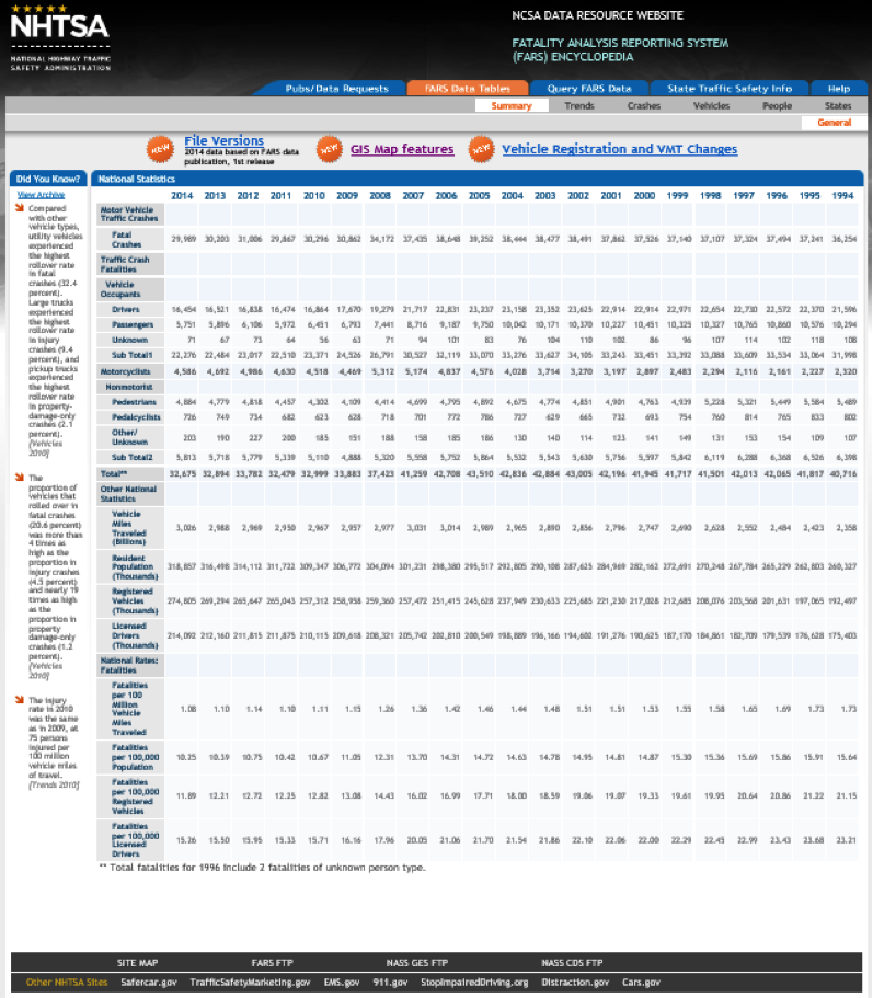
Pennsylvania Crash Information Tool (PCIT)
Some states make crash data available to the public and other interested parties via a web portal. As an example, Pennsylvania makes crash information available via the Pennsylvania Crash Information Tool (PCIT) [82].
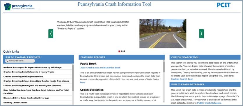
Many of the reports on this site are similar to those in FARS. PennDOT is in the process of adding mapping capabilities to the next version of PCIT scheduled for release in the spring of 2017. Similar to FARS, PennDOT also makes raw crash data available. The PCIT site simply guides users to the PennDOT’s GIS Data Portal [83] for this data.
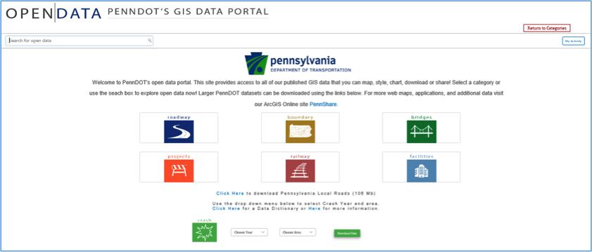
Pennsylvania crash data is available from 1997 to 2016. Differences between the FARS crash data and PennDOT’s crash data include:
- crash data from PennDOT include all reportable crashes and not just fatal crashes;
- crash data from PennDOT include many more attributes or “flags” which can be used to filter the crashes;
- PennDOT’s GIS Data Portal provides very limited querying options (year and county only) and, consequently, the burden is on the user to filter the data to meet their needs.
GIS Uses and Benefits in Highway Safety
As we learned in Lesson 6, spatial technologies are used to locate crashes and perform crash analysis to locate crash hotspots, otherwise known as crash clusters. Spatial technologies also play a critical role in expanding network screening to include roadway characteristics and traffic data in addition to historic crash data as called for in the HSM. Spatial analyses not only help in identifying priority sections of the roadway for safety improvements, but they can also be used to determine the countermeasures which are most likely to be effective and to assess their impact once they have been in place for a period of time. Finally, and perhaps most importantly, GIS plays a huge role in vehicle to vehicle communications and autonomous car technologies. These initiatives promise to have revolutionary impacts on highway safety and make the goal of 0 fatalities seem not so far-fetched.
Optional Reading
In August 2013, FHWA published a document titled Assessment of the Geographic Information Systems’ (GIS) Needs and Obstacles in Traffic Safety [84]. In the document, FHWA identified some of the challenges states face in collecting and integrating crash data in addition to some of the opportunities GIS offers to address these issues.
7.3 Getting to Know a Transportation Organization
This week, you’ll take some time to get to know the National Highway Traffic Safety Administration (NHTSA - pronounced "NITS-uh”). NHTSA is an agency within the USDOT responsible for reducing deaths, injuries, and economic losses resulting from motor vehicle crashes. The agency was created by the Highway Safety Act of 1970 to administer programs that had previously been the responsibility of the National Highway Safety Bureau.
Dr. Mark Rosekind was the NHTSA Administrator under the Obama administration. Take a look at a 37-minute presentation (below) he gave at the Original Equipment Suppliers Association [85](OESA) 2016 annual meeting. Also, spend some time reviewing NHTSA’s 2016-2020 strategic plan titled “The Road Ahead [86]”.
Video: NHTSA Administrator Dr. Mark Rosekind's presentation at OESA Annual Conference, Nov. 2, 2016 (37:36)
NHTSA Administrator Dr. Mark Rosekind's presentation at OESA Annual Conference, Nov. 2, 2016
PRESENTER: Please help me welcome Ann Wilson.
[APPLAUSE]
ANN WILSON: Good morning, everybody. And thank you, Julie. I also want to thank the board members of OESA and the entire membership for allowing me to participate in this great event today.
So let's take a look at this. Safety regulations, V to V, automated vehicles, AEB, NCAP, energy policy, cafe and emissions requirements, cybersecurity, NAFTA, new trade proposals with Asia and Europe, and IP protection. These are just some of the issues that are affecting the members of OESA as I stand before you today. These are issues that'll affect us this year and in the year to come.
Today I want to take a few minutes and focus on three of these issues. Safety, technology, and jobs. First, let's talk about safety.
Let's be very clear about this. All the suppliers gathered in this room are committed to safety. And that commitment has taken on a real sense of urgency nationwide.
We are witnessing a very troubling trend. In 2015, over 35,000 Americans lost their lives on the nation's highways. This was over a 7% increase over the previous year. But if you take a look at the National Highway Traffic Safety Administration's data for the first six months of this year, that increase continues with a 10.4% increase in fatalities for the first six months as compared to 2015.
We all know that automated vehicles will transform transportation. This is especially true when 94% of vehicle crashes are caused by human error.
For those of you who've never heard that statistic before, again, think about that. 94% of vehicle crashes are caused by human error. The promise of virtually eliminating motor vehicle crashes and expanding personal mobility to more individuals and will dramatically shift how society sees transportation.
And make no mistake about it. The members of OESA are at the forefront of this transformation. Our industry is reviewing the automated vehicle policy that was released by NHTSA in September, and we are preparing official comments for submission on November 22.
In our comments, we will be advocating for a balance that provides opportunities for suppliers to work with OEMs on innovation and not stifle it. We are heartened to see the agency create a model state plan that should go a long way in providing a federal road map rather than multiple and differing state laws.
In addition, NHTSA is also focusing on an opportunity for expanded use of the exemption interpretation process. And I know this sounds like legalese to many of you, but this could be a great benefit for emerging technologies to get needed on the road experience.
We are also anxiously awaiting the final decision by the Obama Administration to update the new car assessment program, or NCAP, to include advanced driver assistance programs. The safety benefits of these systems could be immediate because these vehicles and these technologies are on the road now. MEMA studied last year with BCG-- estimated that 10,000 lives could be saved every year if the fleet had a widespread adoption of these technologies.
So let's move, then, to technology. NHTSA last week released a document that I would encourage each of you to read. It's a cyber security best practices for modern vehicles. It is only about 25 pages long. It is actually a fairly approachable document and I would encourage you to read it.
The document states in no uncertain terms that suppliers and OEMs are required-- required to ensure the systems are free of unreasonable risk of motor vehicle safety, including those that may result due to the existence of potential cybersecurity vulnerabilities. This goes on to outline their objectives for the industry including implementation of proactive and preventive measures, real time hacking detection measures, and real time response method assessment solutions.
NHTSA expects the entire industry, particularly all manufacturers developing or integrating safety critical systems, to take part in these efforts. This is not an OEM or a tier one supplier issue only. NHTSA has made it clear that the entire industry, all suppliers, vehicle manufacturers, aftermarket and new technology providers, have a role.
Your DC team is working closely with Brian Doherty, the MEMA CTO and drafting comments to the best practices. But I would also encourage each of you, just as Julie was encouraging you before, to be involved in these discussions.
Finally, let's discuss jobs. MEMA just completed with IHS an updated economic footprint study for the United States. The results were not surprising, but they are remarkable.
Motor vehicle suppliers directly employ over 871,000 Americans. Of that number, 524,000 are jobs that are directly tied to light vehicle manufacturers.
So those of you who have been patiently listening to me discuss automated vehicles and cybersecurity and are thinking that is not what is utmost on your mind, think of those job numbers. How did they impact the US workforce?
Is it worker training? Is it new requirements? Is it job retention? Is it trade? And let's work together to address those issues.
So thank you for your attention to me. But then I want to move on to the reason why we're all here today.
This morning, I have the great honor of introducing the administrator of NHTSA, Dr. Mark Rosekind. Dr. Rosekind is going to give us the benefit of some of his thoughts on some of the issues that I've discussed and a few more, I'm sure.
And then we will have a chance to take some of your questions. And I hope you keep them coming in. We could have a good dialogue about what's to come. So please join with me in welcoming Dr. Mark Rosekind.
[APPLAUSE]
MARK ROSEKIND: Good morning. The full intro is I'm a sleep scientist by training, so when I come in for a morning session and I say good morning and I only hear three voices, either more caffeine or something else. You ready? Let's do it one more time. Good morning.
AUDIENCE: Good morning.
MARK ROSEKIND: Great. Thanks for being here. What I'm going to do is cover three things this morning. I'm going to talk about the safety challenges which Ann just did a great job, but I'm going to be even more specific about the numbers. It's the context for why NHTSA has focused on some of the specific activities we'll talk about this morning.
Second, we're going to talk about our three lanes to get to zero fatalities on our roadways. And then three, we're going to close with talking about what the opportunities are.
Before I do that, something that I always get in trouble for because I can't tell where they are is if you would just join me for a moment, I want to introduce-- we have a very senior NHTSA team that's here. Would you stand because I know you're in the room?
Thank you very much. There's Nat, Allison, and Paul Hemmersbaugh, associate administrator, our director of government affairs, and chief counsel. I say that because afterwards with questions, senior leadership at NHTSA. I hope you get a chance to engage with them, please. Thank you. I'm in trouble later.
Ann's already got us started with this, but there are some numbers that everyone at NHTSA knows, starting with this one. 35,092, the number of lives that were lost on our roadways in 2015. Everybody knows that exact number because every one of those numbers is a father, mother, brother, sister, co-worker, friend. Every one of those is an individual life that we cannot bring back.
Why this is so significant is because last year we clearly have identified an immediate crisis. So Ann mentioned this. Last year, 7.2% increase in the number of lives lost. That is the largest percent increase in 50 years that we've seen on our roadways. Just to put it in perspective, over the decade before that, we saw a 25% drop in lives lost.
What does that mean? That means last year we lost 1/3 of that progress in one year. So far, the six month estimate, which again, these numbers come from us, we're looking at a 10.4% increase for the six month number. This is immediate crisis that we have to deal with. But one of the challenges we have is also look at this as a long term challenge as well, which we will talk about.
This is the number-- Ann mentioned this. NHTSA data clearly shows when you look at the last event, the last cause right before a crash occurs, 94% of the time, it's the human. This is part of the reason there is so much excitement about the technology innovation that's going on.
Can we get to all of that 94% through technology? Unknown. But the key is, look how large that opportunity is.
And just to give some perspective on this, and you folks know it, so that leaves us 6% of the other crashes. So all of you know the headlines related to defects, recalls, et cetera. What percentage of crashes does that account for?
If human behavior, human choice, human error, is 94%, how much is related to defects and recall issues? Anybody know? 2%. Why do I tell you that?
Because that 2% sure gets the headlines, right, while the 94%, which is mostly us because we're all brilliant drivers-- it's the other folks we have to worry about. But it's the 94% that really represents the opportunity where these advanced technologies can really make a difference for us.
When you think about it, though, what's the only acceptable goal for us? It really is zero. And especially as my clock is ticking down, I get more bold and basically say, there really is morally, aspirationally, no other goal we can have. No one has a right to decide, above zero, what would be acceptable. Only zero is acceptable.
The challenge is, when are we going to get there? And what do we do to actually get there? And we're going to talk about NHTSA's three lanes in just a moment.
So one of the things that we've done over the last couple of years is basically work in these three areas. And so I'm going to go through each one of these briefly to give you a sense of the activities that are going on. And one of the ways that I'm going to end, I'll tell you now, we are in this together. And so when I say industry, it is everybody.
So Ann, and Julie, sometimes when they talk, it's like, do we-- where do we need to highlight the supplier side? You're just included, folks. There is no exception for you. You're just included. This is the entire industry and you are part of it, which is why talking about this stuff with you here is just a great opportunity.
So let's talk about proactive vehicle safety just to start with. And what I want to do is just highlight-- in the last couple of years, we've tried to make this very dramatic change. For 50 years, NHTSA and the industry has mostly been reactive, right? And that's what you see up here, is the traditional approach.
So what you're going to try and do is survive the crash, mitigate it if you can, as opposed to the proactive approach which is a transition we've made over the last couple of years, and that is basically avoid the crash altogether. Prevent it. So I'm not going to go through all of these, but the whole idea, again, don't fix the defect after the fact. Instead, you want to prevent. That's what proactive is.
So proactive vehicle safety is something that's under way. I say that because we've already seen some really great successes. Many of you are familiar with our proposals to upgrade NCAP. That started at NHTSA in 1978, and really, it's been enhanced a bit. But really what we've done is proposed the most significant upgrade to that program in almost 40 years.
One of the things we did was put an emphasis on 100% recall completion. A point we have made is that if you identify a defect but you don't get those remedies in place, you still have a problem. The safety risk will continue to exist. And part of the problem previously, of course, is that everyone said, well, 70% is the average. What do people go for? They went for the average.
And I bring this up because just two days ago, we put out a press release. Volvo commercial trucks, 16,000 vehicles with a steering column problem, extremely severe. And after about nine months with FMCSA, with NHTSA, they had 100% recall completion on those 16,000 vehicles before any negative outcomes. No bad crashes, no injuries, no fatalities, all of that done before anything bad happened.
So it can be done. And that's why, literally a press release a couple of days ago, to highlight the success there.
The other thing I just want to highlight here-- AEB, really important. Automatic emergency braking. Because what did we do? September 11 we challenged the industry and said, what can you do to try and make that a standard technology on vehicles?
This is democratizing these technology advances in safety. Rather than just have it a high priced option on our high priced cars, how do we make it standard? We announced that in September, but then in March was able to actually bring forth 20 global automakers representing 99.6% of the new market, are going to make AEB standard by 2022.
Why that's so significant is that was without a regulation. And that is most significant because regulation probably would have taken us three to four years longer. You can count the lives saved, injuries prevented, crashes prevented, by coming out with that collaborative approach rather than waiting for the regulation.
And so another point is the 18 of those global automakers have also come together for some proactive safety principles. And they've been applied already, things like 100% recall, collaborating on cybersecurity.
Let's talk about the second lane, highly automated vehicles. You really can't look at any media today and miss this, right?
So what I want to highlight here, though, is this really epitomizes the proactive approach. The top there is survive it, mitigate it. The bottom is avoid a crash altogether. And that's what we're seeing now.
One of the things that's in the policy I'm going to talk about in just a moment is we have adopted basically to say, let's have the five levels of SAE automation. They're changing recently. But there used to be a NHTSA scale, an SAE-- now it's all SAE.
But I put this up because one of the things that's critical for everybody is to realize, when folks start talking autonomous vehicles, new technology, there's all kinds of different pieces to that. That's what this is and the next slide show you.
There are five different levels of automation. And they represent not just how the human's involved, but how much the operating system, the car, is monitoring the vehicle as well as the environment.
And I put this up because one of the classic questions is, when are autonomous vehicles going to be on the road? People love to forecast this, et cetera. And one of the things I like to say is this stuff is already here.
So for example, here are nine different technologies that are already available on vehicles. I'm not going to review all these, but when you think about it, when is this technology coming? It is already here.
And what's interesting is these are just nine different ones that are available now. So again, when you say, when is autonomous driving here? Well, a level five fully autonomous that you can go to a dealer online and buy one? That's not here. And I love watching everybody predict when it will be. But we'll see how that turns out.
But I put these nine up because I also wanted to highlight, there's all kinds of other technology innovation going on, like this. A driver alcohol detection system for safety. So here's the 10th one. This has gone from research-- we've just spent some time accelerating toward deployment on this.
This basically has two sensors. One, air. So if you're 0.08, it will actually pick up alcohol content just from breathing in the vehicle. And the other is a touch sensor. So through the skin, it would actually pick up if you're 0.08, preventing that vehicle from starting.
So a lot of people who are into drunk driving that understand the issues here, think of DADS as literally the seat belt for drunk driving. So while we talk about the autonomous driving part, the other piece is huge other safety opportunities here as well.
Another thing that we're still working on and have fingers crossed to see is vehicle to vehicle communication. So a lot of people talk about automated vehicles, but connected vehicles really represents-- those two together, automated and connected, really represent the safest, most efficient, most productive, most effective for everybody system. And I put that up because you can see here, when cars can communicate and trucks can communicate with each other, the infrastructure, pedestrians, we're talking about an overall much safer system.
So one of the things, just with some of our data looking at a couple of applications with the intersection, a left turn assist, or a through the intersection detection, you're looking at non-impaired driving crashes, potentially eliminating 80% of those, just with those two applications of vehicle to vehicle. So it's not just automated, but it's connected systems as well. And now we're not just talking vehicle to vehicle, but we're talking the whole system, infrastructure as well as pedestrians, and V2X because who know what else is out there?
But that's why in this realm, and it's been mentioned, on September 20, we came out with the Federal Automated Vehicles policy. So it was in January that Secretary Fox actually announced that President Obama was proposing a $3.9 billion over 10 years to look at vehicle research.
But the other thing the secretary said was in six months, we're going to come out with a policy to address this issue. And that was really significant because up until that time, there were a few pages, if you will, about some guidance, some thoughts, et cetera. This really is a comprehensive approach to dealing with automated vehicles.
So this is the approach we have. First of all, everything we talk about, safety is always at the top of the list. So it's about safety first. That's going to be critical for any discussions you have with us, any actions we take.
The other is-- again, this is a model for proactive. So the framework that's proposed here-- people were shocked, frankly. This document's 112 pages long. What most people expected was thousands and thousands of pages of regulation. We did not take that approach.
The secretary liked to say, we're writing the Declaration of Independence, not the Constitution. So it's a framework. That's why it's only 112 pages. And it's not only the proactive part, but the ideas to facilitate innovation.
If we just prescribe, this is the way everything has to be designed, tested, deployed, that puts everybody in a box. Instead, we're looking for everybody-- and there's a 15 point safety letter everybody's probably heard about. And basically what we're doing is inviting innovation.
So when we've got five people in the front row here, we're hoping that we'll have five different approaches to those 15 items in the letter. That's how you nurture, support, and facilitate innovation rather than saying, all of you have to be in the same box.
In fact, if you think about it, people have been asking, is there a rule-making roadmap here? Well, what all of us would want is be as innovative as you can, send in those lists, show us the innovation, bring the data, and at some point, there's going to be some best practices. What's that based on? Well, that's based on one, or two, or at the top of the list, the best data that shows the greatest safety.
At some point, that best practice would probably be the basis for rule-making, would a different path to take than just coming out with rule-making that could take years and years. And that's why the bottom line I'm going to highlight, there's a lot about data in there, but nimble and flexible I put in there because I think it's pretty critical for everyone to realize-- if we took 6 to 10 years for regulation, by the time it came out, everything from a technology standpoint would be generations too late.
And so part of what's really critical here is to have nimble and flexible built into this, which is why a commitment was made to review this policy and update it on an annual basis. So these are the four elements in there. I hope you've had a chance to read it all. There's no quiz, so you don't have to worry about that.
But it's a pretty straightforward read. Vehicle performance guidance-- again, there's a 15 item safety checklist, basically, a letter that has to be sent in. What does that do?
Proactive means we actually have people looking at safety before anything gets on the road rather than our usual reactive, only looking at things afterwards, when there is a problem. There's a model state policy. What everybody talks about is a patchwork of laws and policies across the country.
We put-- just slam on the brakes here. It would just freeze everything that's going on. And so what we have is a model state policy which very much focuses on what the federal role is versus what the states role are. And we're very clear.
States actually don't have to do anything in this area. If they choose to, we identify some areas they could actually address if they wanted to do that.
The last two have to do with basically tools, authorities, and our regulatory things that we have available to us right now. So we look at the current ones, in particular, we talk about interpretations and exemptions. I want to highlight that because it can often take years to get an interpretation or exemption through the agency.
We actually made a commitment for simple, straightforward interpretations, to get those done in 60 days. Complex ones done in 90 days. Exemptions, for a simple one, potentially in six months. Why are those critical?
Means we have tools now that you could use fairly quickly to get stuff on the road for different kinds of field operational tests. Collect the data to show whether your innovation is really going to make a difference or not.
And then the final section is looking at, what's the future hold? Again, for 50 years we've been reactive. If we want to look to the future, what are 12 different things that we might be able to use? And just to be clear, we don't actually propose anything. We just identified 12 that need discussion so we can figure out what the future will need for us to get these accelerated onto the roadways.
So here's another number that is really important. We actually did a study looking at the last 50 years of 14 technologies that are out there. And seat belts are at the top, airbags are number two. 613,501 lives have been saved by technology.
We know technology can make a difference. And we know it can save lives. This is what our excitement is about.
Now, is that the only thing we need to be focused on? Absolutely not. And that's why this last lane has to do with us a human, that 94%.
And NHTSA's already been involved in this tremendously. We have a huge number of programs focused on our behavior. These are national programs that hopefully all of you are familiar with.
What's clear, though, is that we have to wonder, what are we going to do? Well, it ends up we actually published something that talks about the strategies at work. There are about 120 strategies in here. And we know what actually works.
So for the immediate crisis, the rise that we see going on now, we know that there are strategies that will work. But is that the only thing we can do? That's this guy, right? If we keep doing the same thing but expect a different outcome, they call that insanity. Thank you, I heard you. You're really there.
So we have an immediate crisis, we can do the stuff we know that works but if we keep doing that, we're never going to get to zero. And so that's why September 20 we announced the autonomous vehicles policy. And then on October 5 we actually talked about a new Road to Zero coalition.
And it has two specific goals. First is the immediate near-term. Let's apply all the stuff we know that works. But we're also identifying specific money, specific support for innovation. Where to identify the gaps where stuff can be improved or new things can be applied to deal with the immediate increase in fatalities that we're seeing?
But really, the longer term challenge is going to be addressed by the second bullet there. And that is, we have a group that's coming together to create a 30 year scenario based plan on how to get to zero.
They're sweet and started with zero as a goal. We have vision zero toward zero, a lot of different programs focused on this at states, at city level. What has been missing, really, is putting all of those together and having the long term plan.
People are just counting lives lost, crashes, year by year. We need a 30 year plan. And it starts with a scenario that says you wake up in 30 years and no one lost their life on our roadways. And then you look at the milestones to get you there.
So that's why this effort is really very different. Deal with the immediate crisis. It'll take about 12 months or so, at least, to come up with that 30 year plan to figure out how we get to zero.
That's being done with three different agencies within DOT. This has never happened before. So it's not only NHTSA, but it's the Federal Highway Administration, Federal Motor Carrier Safety Administration.
So the three surface modes at DOT have come together. We are partnering with the National Safety Council to do this. And I mention that because while those groups are the coordinators for all of this, we already have 75 organizations participating. This is all inclusive.
So whether it's used in individual company, OESA as an organization, everyone needs to participate. Everyone needs to take part in this. The only way we get it to zero is if all of us are participating and take responsibility.
Last two slides. First, this one. For the last two years, NHTSA's really been going through a very significant transformation. The first thing at the top there is we've had three specific things we've focused on just strategically. That is, fix the things have been broken, and I would say that's both within NHTSA but within the industry that we can. We're talking about a pivot to proactive. And I've been giving you all kinds of examples through this discussion.
And the other is, for all of us, we have to create and then own the future. We can't just wait for all of these things to happen to us. And so these three strategic approaches have been what NHTSA's actually actively been pursuing over the last two years.
And what you see below that are 12 concrete examples of things that have been accomplished and initiated over the last two years. I put at the top there the Federal Autonomous Vehicles policy and the Road to Zero. Because those two, to me, are the capstone of the last two years.
They epitomized what proactive means. And for all the work we can do in Road to Zero, autonomous and new technology innovations will be a critical element for us to get there faster than if we just do the stuff that we've been doing for a long time.
So this just gives you an example of some of the very concrete things that NHTSA's been doing. But that's why I said the last slide-- with these three lanes, one of the things I've been highlighting to everybody, there is a moment going on with people not just focused on proactive but the actions that need to be taken for all of us to be able to really reach zero lives lost on our roadways.
So I think for everyone, and this is what I started with, our suppliers, different tiers, different than the OEM-- we're in this together, folks. There are things in the AV policy that apply to you. Everyone who rides their bike, walks, which is everyone here, is in a vehicle, whether it's commercially or your own, everyone is invested in this. This is your life we're talking about, and your family, and your co-workers.
So we are in this moment right now for everyone to figure out how you're going to travel, in one lane, in all three lanes. My bottom line is, though, that this is a responsibility we all share. 35,092 should be completely unacceptable to all of us.
100% of those are preventable lives lost. And we cannot bring them back. It is tragic. That is the equivalent of a 747 crashing every week for a year.
And the increase last year, five more jumbo jets went down. If that happened in the United States in one week, that would be headlines for three months. If it happened a second week, we would shut the aviation system down until we figured out what was going on.
And yet we accept not only that high number, but increasing numbers like it's OK. It's part of the risk. It's part of the cost of getting the mobility we have today. It should not be.
And we are in a moment where we can make not just a big difference in that, but go beyond safety to mobility and sustainability with all of the opportunities in front of us.
So please join us. Please join with your colleagues. This is a path that we can only attain if we do this together. Thanks very much. I'm going to look forward to speaking with Julie and Ann. Thank you.
[APPLAUSE]
[MUSIC PLAYING]
PRESENTER: Great, thank you so much. Thank you for being here. We appreciate your candor and speaking to this audience of suppliers. It's so key.
I need to start with a question. It rose to the top very rapidly in terms of the questions as we have them coming in. And it deals with Tesla.
And the question is, really, with the Tesla death that unfortunately occurred with their beta system software, Tesla instructed the drivers of their vehicles to simply turn off that software. The question is, if it was a more traditional OE, it would have probably been a recall. Why the difference? And what was your thought process when you saw that occur?
MARK ROSEKIND: I think we're going to get to the next question really quickly because NHTSA actually has an investigation into that right now, which is why I can't comment on that in any way. But I think that gives you an indication-- as soon as we heard about that, we gathered information and initiated investigation. So that's going on right now to determine specifics from a NHTSA perspective.
PRESENTER: OK. The next question that we have is really-- I thought it was very insightful. If you had two more years with NHTSA, what would your priorities be?
MARK ROSEKIND: Great question. So why that's so interesting personally is because I finished five years at the NTSB, came to NHTSA knowing that I only had two years. So I warned everybody, we got to sprint. And I don't mind telling you the calendar we're looking at. We are, like, running through the tape through January.
And I'm saying that because why that's so interesting is I think there have been a lot of times where I come up against something and say, you know, if you had four years, you'd be putting that not just on the list. You'd be going after it.
So I think there are-- my highlight would be that I think what I showed, our 12 things. A lot of those are initiated. But it's delivering long term on them. And if we had four years, we'd be doing that a lot more solidifying way.
So one of the things I-- story I tell is when I met the secretary about this position, he said, Mark, in two years we're not going to fix it all. We're not going to get it all done. But we could put some big markers down. Set the path. So I think part of what would be done was making sure those markers were deep and we were following them to the safety goals that we've established.
PRESENTER: And so Ann, how does that-- those goals, if you will, the markers that have been set down-- how does that line up with what you see as suppliers' priorities for the coming years?
ANN WILSON: Well, I think a couple of things. As I look around the audience, there's a lot of you I interact with on a lot of basis and you interact with other folks on the DC staff and with other people in your teams, too.
But there's a whole bunch of you who are very involved in the safety process and fuel efficiency who don't interact with Dr. Rosekind's team, don't interact with us, and we need to change that. So, I think that's one piece of it.
I do think we have been-- and I know you've heard this from me before-- want to make sure that suppliers are fully involved as you develop these policies and guidelines because suppliers have a unique position on them and I think it's important for us to do that. But that's incumbent on both us and on the agency. It's not just on the agency, but it's incumbent on us to bring information and data and our viewpoints to the agency. So, I would think that would be my first one for two years.
MARK ROSEKIND: Can I comment?
PRESENTER: Yes.
ANN WILSON: Please.
MARK ROSEKIND: If you didn't get the message, this opportunity is for everybody. Ann and I have talked about this a lot. Anyone who's sitting there thinking, well, but that doesn't apply to me, wrong.
Everybody, whether you think or not that this is specifically in your lane, the reality is, whether it's personal or business, you have a role in this. And the only way we're going to get to zero is through all doing this together. And so the opportunity part is for everybody. And anyone who sits back and says it doesn't touch them is wrong.
You got to participate in some way. And the other thing, thanks for mentioning that-- because the policy that's out is still in a 60 day comment period. So you can actually put comments into the docket. By November 22 it closes and we have a November 10 meeting that just got announced, it's on our website, that's going to actually look at two things.
One is overall comments so you can come and make a few minute testimony, basically, about the overall policy. And the second part is we're looking for information about creating a template for that safety letter. So November 10, same thing. You could come and give us input of what you actually think belongs in that safety letter. And we're doing those on the 10th so we can do that before we close the 22nd comments.
And one more thing. When you read the policy you will see we actually have 23 next steps that are outlined in there. So this is not a, make the comment and you're done. This is nimble, flexible. There'll be many other opportunities which is, take advantage of it.
PRESENTER: We have a number of questions that have come up with regard to the increase in fatalities. The question as to, what do you think is causing that? How do we stop people from texting? So what do you think the causes are? And if it's texting or being on your phone or distracted that way, what's the thought process at NHTSA behind that?
MARK ROSEKIND: I think we've been looking at two pieces of it. One is, if you look at the data in more detail, you realize that vehicle miles traveled has gone way up.
And some of that is good because what it represents is higher employment, younger people getting out there, better weather. I mean, I saw this data. It's like, better weath-- yeah, people are out. They've got more disposable income. And about half of the increase could potentially be due to that.
The other half, unfortunately, are all the problems we already know that exist. So things like distraction, drowsy driving, speeding, drunk driving-- drug driving is becoming much more of a significant issue. All of those things that we know are classic. Basically, when you put people on the road, they're at risk for all of these things we already know and they just take more lives and create more crashes.
ANN WILSON: So Julie, can I say one thing?
PRESENTER: Please.
ANN WILSON: MEMA worked with many of the companies here, and many of the companies here have worked individually on a lot of the technology that's currently on the road. And we've worked very closely with Dr. Rosekind and his staff on this.
And this is one reason why-- I know I went through in my five minutes very quickly, but why the new car assessment program is so important. We really think it's critical for us to get information into consumers' hands so that when they're purchasing a vehicle they-- you've got the AEB but you've got blind spot detection. There's other kinds of technologies that are out there that maybe can't get to the root cause of some of these accidents but can help prevent some of them.
So I encourage those of you to watch this as it progresses, watch NHTSA's views, DOT's views on this, and watch our views on this, because we think that this is a very important-- the idea of an automated vehicle is really tantalizing. But there are concrete steps that we really think that we can take together now.
PRESENTER: I have one last question here and then I'll offer you some time for closing comments if you have any. But this question I thought was very interesting. Are we seeing an increase in traffic deaths related at all to age, either aging at the more senior or the younger side of it?
MARK ROSEKIND: I didn't pay you to say that. Because it actually ends up-- tomorrow we have an older driving event in Washington looking specifically at this issue. Because there have been a lot of claims about that. But as a scientist, I'm always like, claims and hypotheses are one thing. Data, something different.
So tomorrow we're actually going to be looking at not only what does the data tell us, but what are the new, innovative things we could do to address that special group? It ends up-- folks that are older have, like, a five times higher risk. And that's just because anatomy and physiology is different. Their body reacts differently in a crash. And so we're going to be looking at that tomorrow, actually.
PRESENTER: Any comments that you'd like to make as we close?
MARK ROSEKIND: I think I would just close with-- the slide about NHTSA's transformation is really to share the opportunity with everyone that our couple of years have been focused on such a significant shift from 50 years of being reactive to trying to get proactive. Let's avoid crashes and all the problems.
That's pretty major. It's going to be a pretty significant culture change for everybody. And you can't do that just in two years. That's why you need everybody involved. And what I'm hoping is that what NHTSA's done is work with folks, all the industry, and safety advocates, and everyone else, you can think of, to get those markers down.
PRESENTER: Ladies and gentlemen, please help me thank both Ann and Dr. Rosekind. Thank you for all your candor.
[APPLAUSE]
| Strategic Goal | Strategic Objectives |
|---|---|
| Safety |
|
| Proactive Vehicle Safety |
|
| Automated Vehicles |
|
| Human Choices |
|
| Organizational Excellence |
|
Credit: THE ROAD AHEAD, National Highway Traffic Safety Administration Strategic Plan 2016—2020 (USDOT, NHTSA October 2016)
A few of NHTSA’s areas of focus are briefly described below:
Vehicle Safety Ratings and Recalls
NHTSA plays a large role in accepting and tracking vehicle safety complaints which can ultimately lead to safety recalls. They also administer the New Car Assessment Program (NCAP) which assesses and scores vehicle models using a 5-star safety rating. Safety rating and recall information [88] is compiled and made available to consumers. Using this information, consumers can quickly determine how specific vehicles perform in front-end, side, and rear-end collisions in addition to rollovers. NHTSA also compiles safety information on car seats, tires, and other equipment.
Data-Driven Approaches to Crime and Traffic Safety (DDACTS)
DDACTS is a model which NHTSA developed in association with the Department of Justice (DOJ). It uses the temporal and spatial analysis of crash and crime data to identify the optimal deployment of highly visible law enforcement personnel and vehicles. Detailed information about the model is available in the DDACTS Operational Guidelines [89].
National 911 Program
The purpose of the National 911 Program [90] is to promote and coordinate 911 services across the U.S. NHTSA is currently promoting and rolling out the Next Generation of 911 (NG911) which will modernize 911 systems based on advances in technology which have occurred since 911 was first put in place 50 years ago.
Office of Vehicle Safety Research
The Office of Vehicle Safety Research is a NHTSA Office that develops and implements research programs designed to reduce crashes, fatalities, and injuries. Some of their research activities can be found here [91].
National Center for Statistics and Analysis (NCSA)
The NCSA [92] is an office within NHTSA which provides analytical and statistical support to the agency through data collection, crash investigations, and data analysis. One of NCSA’s responsibilities is to maintain and enhance FARS. They also produce many useful and interesting publications summarizing information gathered by NHTSA [93].
7.4 Getting to Know Each Other
This week, you’ll have a one-on-one chat with one of your classmates (or me) as per the schedule you were provided in Week 1. The discussion should be at least 30 minutes in length. If it’s the first time you’ve chatted with each other, spend the majority of time getting to know each other. Otherwise, focus on discussing the lesson content.
7.5 Webinar for Next Week
Next week, we'll hear from 2 speakers.
Speaker #1
Our first speaker will be Mr. Jeff Roecker. Jeff graduated from Penn State with a degree in Geography and joined PennDOT in 2008. Jeff plays a lead role in the Department's Crash Data Analysis and Retrieval Tool (CDART), and he is the project manager for PennDOT's Strategic Highway Safety Plan (SHSP).
Crash Data Collection
FHWA requires all states to maintain a database of crashes in order to support the analysis of crash locations. There is variation from state to state on how they define reportable crashes, how they collect the information and how readily they share the information. Many states publish annual summaries of crash data for the prior year and also provide trending information for various crash statistics. The Pennsylvania Department of Transportation (PennDOT) publishes an annual report entitled Crash Facts and Statistics. The 2016 version of this publication can be found here [94].
Crash data is important to state DOTs for a number of reasons. First, without this data, an agency doesn’t know if things are improving. Second, this data can offer clues to where safety improvement or countermeasures are most needed. Crash patterns can also be used to help law enforcement design initiatives associated with seat belt usage and checkpoints for impaired drivers.
Law enforcement officials are generally responsible for reporting crashes. In Pennsylvania, the Commonwealth of Pennsylvania Police Officers Crash Report Manual provides law enforcement agencies instructions on reporting crash data including definitions of which types of crashes are reportable to PennDOT. The police use a multipage form (AA 500 [95]) to report crash data. The form captures extensive information about the crash including the location, all vehicles and individuals involved in the crash, the number and nature of any injuries, weather and road conditions at the time of the crash, a diagram of the crash, and statements from any witnesses. PennDOT also provides a detailed reference document known as Pub 153 [96] to help police officers complete the form correctly.
PennDOT also has a web-based system called the Crash Reporting System (CRS) which provides an electronic alternative to submitting crash data. A user’s guide for the system can be found here [97]. CRS is also used by PennDOT to review and validate all data which is automatically retrieved from paper forms which are received from law enforcement agencies. Any meaningful analysis of crash data requires that the data is accurate and complete.
Crash Analysis
State DOTs use crash data to identify locations where there are unusually high crash rates and also to determine measures which will likely lower these crash rates. One of the most useful types of crash analysis, which is used by many state DOTs, is a spatial technique known as cluster or hot spot determination. This type of determination is done using GIS software by stepping along each route and identifying sections of roadway which meet the definition of a crash cluster based on established parameter settings for the analysis.
In Pennsylvania, crash data submitted by law enforcement agencies electronically via CRS or the AA500 paper form, are processed and stored in a system known as the Crash Data Access and Retrieval Tool (CDART). CDART is a geospatial application which allows PennDOT to perform a variety of crash analyses including crash cluster analyses. It performs two basic types of crash cluster analysis. The first is a standard cluster analysis where each road is considered separately. The second is an intersection-based cluster which examines the number of crashes which occur on all associated roads within a certain distance of the point of intersection. One of the other interesting analyses CDART performs is a “before and after” analysis which compares crash frequencies for a section of roadway before and after a safety improvement was implemented to determine its effectiveness. For each of the analyses CDART performs, the system allows the user to generate tabular or map-based outputs. CDART is an internal tool to PennDOT and is not available for public use.
On May 30, 2013, Sharon Hawkins of the Arkansas DOT gave a 42-minute presentation on some of the GIS tools [98] they use to locate and analyze crashes (located below). The presentation was part of the FHWA GIS in Transportation webinar series. The webinar provides an excellent perspective on the importance of GIS in collecting and analyzing crash data. Many states have gone through a similar evolution and set of problems in their efforts to manage and utilize crash data to improve highway safety.
Video: GIS Tools Used to Locate & Analyze Crashes (42:28)
SHARON HAWKINS: [AUDIO OUT] and we have about 16,400 plus miles of state highway. We're the 12th largest state highway system in the nation. And then just a little bit on the topography of Arkansas. A lot a mountainous regions, rolling hills, and a nice flat delta region. A lot of different terrain as far as where we're building our roads, and a lot of different terrain to analyze when we're looking at our crash data. So I want to do a few statistics about our crash data before I go into the tools that we're using.
So here's a chart showing the total number of crashes in the state, and total roads versus just the state highway system for the past 10 years. And you guys can see, about 60% of all crashes in Arkansas occur on our state highway system. 70% of all crashes in the state-- total crashes-- occur in our urban areas. And then 70% of all crashes that happen in the state that have a fatality involved occur in our rural areas. And 2/3 of those are roadway departure related.
There were 550 crash fatalities in Arkansas last year. This next chart kind of gives a comparison on how our fatality rate versus the national fatality rate. And you guys can see, we're just a little bit above what the national fatality rate is. All this being said, with our crash location tool, it's very important for our new initiative towards zero deaths to make sure that we have all the spatial information that we need in order to make our routes safer for our traveling public.
So I'm going to go over kind of past to present-- the different kind of tools that we've used in the past to locate our crashes. And then I'll be introducing our new tool that we're going to use. So we've been progressively implementing new methods over the years. And so for the next few slides, I'm just going to show what we've done from the 1970s through 2011, before the implementation of our new tool.
So in the 1970s, the department was tasked with locating and maintaining all the locations for crash events on the state highway system in Arkansas, and just on the state highway system. So for this purpose, the department decided to record each crash event with that event's county, route, section, and log mile location so they could be found and studied on the highway system, since the system uses the same county, route, section, and log mile set up. And we live by the log mile here at the Arkansas Highway Department.
The department partnered with the state police and local county and city law enforcement to make sure that they could locate each crash with its needed attributes, including an accurate log mile of where the crash event occurred. So we were relying on other law enforcement-- law enforcement that weren't familiar-- very familiar, anyway-- with the log mile system to get a log mile for us.
So this slide shows one of the earliest tools that we would use, which is our county, route, and section map. It only shows the state highway system on the map. Of course, it has the beginning and ending log mile for each segment of highway, and it has a log mile for all the bridges on the map.
So we were asking them to give us an accurate log mile for a crash location based on these maps. You guys can imagine how difficult that was for them. But there was a backup. And we also-- here at the department-- we had crash locator positions. And they had to locate-- relocate-- all those crashes that happened on the state highway system.
So next, we also had our tabular road inventory information in these big books that they were able to flip through. And for each route, wherever it intersected another state highway system, of course, there was a log mile listed, and then events that happened on the route. So a number of lane changes, ADT changes. There were log miles listed for that.
As you guys can see from the picture, very difficult to understand. Our crash locators here at the department could hardly understand it, so it was very difficult for us to think that other law enforcement were going to be able to understand it also. So once again, every crash had to be relocated here at the department, even though we were getting a log mile from our law enforcement.
So we also provided static printed maps, and our workers here would write in the log mile wherever there was an intersection with another route. So we would take these maps. We would hang them up with the city so they would have a static map on their wall to look at to better locate a log mile. But you know, those maps could be out of date, you know, as early as the next day. There's always system changes on the highways. So this is not a very efficient way to get it done.
So next, we offered that we could make these maps-- we didn't have to handwrite anymore. We could use MicroStation. And we could put log miles in where routes intersected the state highway system so they could have a better feel of what log miles were available for them to choose from to report the crash location. Once again, maps could be out of date very quickly. And even though these were available digitally, most cities still relied on their printed versions that were hanging up on their wall.
So in 2004, we realized the power of our linear referencing system and how it could help our crash locators here at the department locate exact log miles of where crashes occurred digitally in our GIS software. So we set up the program with our CAD maps. And we had our linear referencing system on top of those CAD maps so they could see intersecting routes with our state highway system.
They could hover along using a tool called LRS Precision Location. As they hovered along the state routes, they could get an exact route section and log mile of where their point was. Very helpful for our crash locators here at the department. But we couldn't share this tool with law enforcement, because they didn't have the software, and not the knowledge, either, of the linear referencing system.
So still, we were in a continuous cycle of us having to relocate all crashes that happened on the state highway system to make sure we were getting an accurate log mile. And we were lucky. Our Arkansas Geographic Information Office had gotten with the counties, and they had developed a 911 center line routing system for the state.
So thank goodness we had a whole state network that was attributed with road names and such so we could utilize that with our linear referencing system, and they would be able to see the routes, their attributes, their names, to still better identify a crash location. But once again, that was a tool that we could only use here at the department, and other law enforcement just couldn't get to it.
So we also tried, during that time, GPS units. We bought 50 GPS units, sent them out with the state police. We wanted to do a trial period. Maybe they can use these GPS units, take a reading at the crash scene, get a lat/long for that crash, get it into the system. And then we would have a latitude/longitude that then we could convert to log mile for our report. So we tried this for about three months. We gathered the data.
I've heard this from many other states-- when we got the data back and mapped it, a lot of those dots landed in the state police parking lot, or they had moved to the side of the road, so-- in other parking lots where they were. It just wasn't convenient. It wasn't going to work. Not necessarily the law enforcement's fault. They didn't realize how important this was to us to make sure that we had these correct locations. And there was minimal training when we did give them those GPS units.
OK. So just a little bit about our linear referencing system, which was a major player in the tool that I'll be introducing in just a minute. So as I said before, over 16,000 miles of state highways on our highway system-- 12th largest in the nation. And also included on our linear referencing system, over 15,000 miles of other routes eligible for federal aid. So what you're looking at here on the screen is pretty much our functional class system-- so all routes eligible for federal aid. It's what we have currently on our linear referencing system.
So our linear referencing system sure works like most other DOTs. We assign the route with the county route, section, and beginning and ending log mile. The concatenation of the county, route, and section and the log mile information is its unique value, or its primary key field. And then we can map different things from around the department that also have that same primary information, such as job status, information from our road inventory, and of course, crashes.
So updating the LRS, 177 changes were made just in 2012 on the state highway system. We have removed routes, added routes, relocated routes, and often a lot of relogged routes throughout the year. We keep a live version of our linear referencing system open to everybody here, but we also keep archived copies. We started archiving our linear referencing system in the year 2000.
So we can always go backwards to see what the system looked like back then, which is helpful. We just received the 2011 statewide crash data, so we can't use current linear referencing system to locate on. We're still locating crashes that happened in 2012, so we do have to keep these archived copies to make sure that we're locating in the correct year that the events occurred.
OK. So let's look at one of our typical crash reports that we get here at the highway department. It happened on the state system that we have to relocate. Of course, all the information here. You see a little narrative about where the crash happened and a little diagram. This particular crash says it happened on US Highway 82 in Columbia County, section 3b, log mile 2.20. So we're going to relocate this crash and see how the law enforcement did out in the field.
OK. So from the narrative, we see where the red circle is in the middle of the map, that this is approximately where that crash happened. But they said it happened at log mile 2.20, but this route only goes to log mile 1.65. So couldn't have happened. So we're going to have to relocate this. OK. So after our locators got a hold of it, we relocated it to say, now it happened on Highway 79, section 1, at log mile 18.26.
Those are going to be sent back to our state police. The location is going to be re-entered into the database for the correct crash location. So once again, that's a prime example of how difficult it is for our law enforcement to give us the correct log mile. So back in February of 2011, one of our county offices-- Polk County Sheriff's Office called. We just had a big snowstorm. We were still waiting for the snow to go away.
And they said, hey, we need that map that we're supposed to use to locate crashes by log mile on the state system. Can you tell me where that is? So we directed him to the route and section map that they've used. And he said, hey, is there an easier way? And that very day, we sat down, and we came up with an easier way. And we don't blame them for asking.
In this instance, here's a route. It's about 19 miles long. There's no log miles in between for them to guess, so they have to use the little section lines to kind of guess where that log mile could be. And they have 52 different fields of information per crash to enter in. A log mile's not necessarily on their radar as the most important field. So a lot of human error. And then with our locators having to relocate all those crashes, sometimes we weren't getting those locations in in time to really do some real-time analysis with our data.
So, making it easier-- so what we did is we took our linear referencing system that included all routes eligible for federal aid around the state, and we asked our GIS platform-- we asked GeoMedia to put a point every 100 feet along the linear referencing system. So when it did that, each point was populated with the county, the route, the section, and the exact log mile of that point.
So then we say, OK. Well, let's make this a little bit better. Let's attach some of our road inventory data to those points also. So now, with county, route, and section, and the exact log mile of that point, was other information that was going to be very useful to the law enforcement to fill into their reports, also.
Well, then we took the points and we said, hey, let's shove these out to a KML file for display in Google Earth. So we did that through our program. And as you can see from the screen, in the red, we have what's on the state system. In the blue dots, we have other routes eligible for federal aid, or the rest of our functional class system. And you're able to click on those dots in Google Earth and see the exact information that was generated in our GIS platform.
Of course, these are KML files. We can email them out to anybody. You can email them out to family members. They would be able to see. So we started emailing these out to our state police for them to be able to give us a more accurate log mile of where their crash events occurred. And it's just worked out wonderfully.
We also included our city limits, as you guys can see in the top left of your screen. There is a field they had to fill out that say whether or not it's in the city or out of the city. And if it's out of the city, they have to measure how far out of the city it's out of. So we have our city limits available to them. Instead of just being able to locate on main lane, they can now see the log miles on frontage roads and on ramps.
And of course, they have Google Street View available in here to be able to help them better locate where they are in the field. And of course, this allows them-- if they have connections, they can locate right there in their vehicle at the scene of the crash. If there's no time, they can always come back to the office and, of course, use this tool also to locate the incident.
In this case, this is a pretty long bridge that we have here in the state-- the 430 bridge. The beginning log mile of the bridge with 9.87, if you guys can see in the graph on the corner of the screen. So we had a lot of accidents that happened at 9.87 on that bridge.
But as you guys can see, every 100 feet along that bridge, there's a lot of dots. It's almost two miles long. So they're able to give us a more accurate, better log mile when they're out in the field. Not only are the law enforcement outside of the Highway Department using this, but also our crash locators are taking advantage of this tool and now using it to locate those crashes.
So how can everyone use this tool? We can email out the KMLs to everybody. We have FTP sites that's open to the public. Anybody can download those KML files. We also have all these points, or dots, every 100 feet available on Arkansas' GIS clearinghouse called GeoStor. In addition to that, our Arkansas Geographic Information Office offer this data available on ArcGIS Online.
So we have all of our dots in there. There's a link that anyone can click on and go in there and see the same exact information that was offered in the KML files. And also, ArcGIS Online can be used in their smartphones, also. So if they don't have their laptop open, or a good connection, they can also use their smartphones to be able to see that information.
So the use of the LRS location tools, or our new crash location tool, the training and outreach to law enforcement agencies started in June of 2011, so just three months after we came up with the methodology. All of the state police agencies are using this, which account for 25% of all crashes statewide, or about 40% of crashes on our highway system are being located using this tool. And we constantly reach out to counties and cities. Right now, it's just a volunteer basis for local law enforcement to use it. But we have about 42 of those agencies that have started to utilize it, and we've gotten very positive feedback.
So once we have the data, our better locations that we have. Of course, numerous planning studies are done in order to figure out, hey, do we need a passing lane here? Do we need more lanes here? Maybe a turning lane here to make things safer. Maybe some rumble strips.
And then we can also run all kinds of queries, as far as types of crashes, to be able to look for areas that might need to be paid attention to for more safety initiatives to take place. As far as safety initiatives, having this data, having these locations in a more exact location for us, we've been able to prove that different things, such as cable median barriers, need to be installed in more areas around the state. Rumble strips need to be installed, especially on some of our two-lane rural highways where run off the road crashes were very prevalent.
And then we have one more tool that we started using. It's called Intergraph's Incident Analyst. It's been able to help us identify clusters and locations-- areas-- that we really need to pay attention to that we haven't been able to find as quickly without this software. So case in point, this is a study we did in Jacksonville, Arkansas. We had to make a map for our administration so they could see the clusters of crashes that happened in Jacksonville.
The map on the left, you guys can see all the clusters of crashes-- the yellow dots there. This map took about four hours for us to put together. A lot of these crashes happened at the same exact log mile, so the dots are just right on top of each other in our GIS platform. So we exported it out to our CAD. We took those dots. We moved them around so we could produce those clusters.
So once again, about four hours. But with Incident Analyst's hot spot analysis tool in our GIS platform, it took about two minutes for it to generate this hotspot map for us. You guys can see that the two maps compare very well with the clusters. On the right hand side, the hot spots in the red are showing where those clusters are that you guys can see on the map on the left in the yellow.
And then there's also a incident count tool. You can count incidents within any boundary area. So in this case, we're using county. But you can also do cities. We do a lot of House and Senate districts if our legislators want to know where most of the accidents are happening within their jurisdictions.
And there's also a repeat incident tool that we use to run-- this is on a statewide basis, but we can run it on any sized project area in the state. But it lets us know quickly where repeat incidents happen over and over again at the same log mile location so we can really focus on those areas and do some study analysis to find out if there are some safety issues within those areas.
They do have a tool in there also called Change Over Time. It kind of plays a little movie for you, what happens with these incidents. I just did January through June for this. It's in PowerPoint, but once again, imagine it's a movie. When I flip to February, keep in mind that we had a pretty big snow storm this year, so a lot of crashes happened that month.
And there's also temporal reporting. It makes nice charts for us to be able to show where the majority of the crashes happened. So at the top, you see month of the year, in the middle, day of the week, and then on the bottom, time of day-- crashes that happened. And this helps us put together nice figures, especially for public involvement.
We used this at a public involvement meeting. We did hotspots of the crashes. On this particular study segment, we wanted the public to know that we know that there are a concentration of crashes that happen in this area, and it's under study, and we have plans in place to rectify that. And also, we had our temporal reporting on top of that figure.
OK. In the future, a methodology will be in place by June 2013 to include all public roads in our linear referencing system. So from our about 30,000 miles that we have available now in our linear referencing system, approximately 110,000 miles will be included in there. You can see from the figure, in the red, this is about how much we have to add-- about 74,000 miles we're going to have to add for our linear referencing system.
But when that's done-- and we guesstimate in approximately five years-- we'll be able to locate all crashes in the state, not just on our federal aid system, which, the safety initiatives-- there's nothing like having more data to do analysis with to find out what needs to happen.
Of course, the dual carriageway system will be put in place along with that linear referencing system. So each divided highway will have two centerlines, and road inventory will include complete data for log direction and anti-log direction. Right now, we can only map on our linear referencing system based on one centerline. But you guys know, FHWA has asked us to do dual carriageway along with an all public roads linear referencing system.
And in 2014, the Highway Department, along with the Arkansas State Police, will start implementing eCrash, which was developed by the Center for Advanced Public Safety, or CAPS, at the University of Alabama for a paperless, electronic submission of crash reports. eCrash will have an actually map click tool that our law enforcement will be able to use in their vehicles. They'll be able to click on a location. It will give a latitude and longitude of that crash. But they are going to be using our points-- every 100 feet points-- within the map click tool, also, for log mile information.
OK. And this is just to illustrate we're just skimming the surface of what we can do, and look at all the potential that's ahead of us, especially when we get our all public roads linear referencing system in. OK. And contact information right here. For more information on Intergraph's GeoMedia, or Incident Analyst, James O. Brown from Intergraph's. And then more information on eCrash, there's a link on there for you to look at also. And then I'm happy to answer any questions.
Thanks, Sharon. I'm going to go ahead and open up the lines for question and answer.
[BEEPING]
PRESENTER 2: This conference is now in question and answer mode. To alert the speaker that you have a question, press 1, then 0. Each question will be asked in the order it was received.
[BEEPING]
MARK: So you should have heard some instructions. If you've got a question on the phone line, just press 1 and then 0. You can also enter in questions into our chat pod, especially if you're listening through the computer. Let me just quickly see if we've got questions on the phone. No, we don't have any questions on the phone right now. But let me see.
So Sharon, you mentioned that one of the issues that you had rolling out different-- the first couple attempts at something like this, the training seemed to be-- play a role, or trying to understand how the users, especially the state police, were going to try to enter in the information. It sounds like that what you have now, it was much easier. But are there still issues you're running into in terms of getting the--
SHARON HAWKINS: [INAUDIBLE].
MARK: --location information?
SHARON HAWKINS: Well, it's true right now, when they click on one of those dots and see the information they have to enter in their report, they do still have to enter that in by looking at what they see in the crash location tool and Google Earth, and typing it in. So there's a lot of human error in there. But aside from that, we've been constantly checking the locations that have come from this new crash location tool.
And the department's made a decision that as long as they use this tool, which there's a checkmark they can check to say they used the tool, we don't have to relocate those crashes anymore, which means, for us, that we're getting our data-- our crash data-- instead of a year and a half later, we expect to see our crash data eight months after the year ends, instead of a year and a half later. And then we hope in the future, it just comes on faster.
MARK: Mm-hmm, mm-hmm. Because I know a lot of states are-- that's one of the issues, is trying to either make it easier for the-- especially the state police. They're involved in entering a lot of this information-- making it easier for them to somehow put that in.
SHARON HAWKINS: Right. And that's why we're looking forward to eCrash with the map click tool. It's a paperless system. When they click, a lot of our road inventory information, and of course, that log mile information, will automatically be entered into the report through the eCrash system.
MARK: Mm-hmm. Looks like we have a question. A user that uses ArcMap, they want to know--
SHARON HAWKINS: Right. so-- yeah. We do have ArcMap here at the Highway Department. But GeoMedia is our GIS platform. So I hope maybe that somebody else that's on the conference would be able to answer that question. I know that ArcMap has the capability for hot spotting, but I am not quite sure exactly where that is.
MARK: How did you learn about the Incident Analyst product? How did you find out about that?
SHARON HAWKINS: Intergraph, actually, was advertising it. A lot of-- like a crime location tool where incidents happen over and over again. And then they worked with Ohio data, and they kind of started advertising it as a hotspot tool for crash analysis. So when we saw the presentation, we knew that it could be a good tool for us to be able to take advantage of for hot spotting.
MARK: Mm-hmm. Let me just quickly check on the phone lines to see if we've got any questions.
AUDIENCE: [INAUDIBLE]
AUDIENCE: [INAUDIBLE]
MARK: Hello?
AUDIENCE: Hello?
MARK: You've got questions? Yeah. What's your name?
AUDIENCE: This is David Lawler with TDOT.
MARK: OK. What's your question?
AUDIENCE: I think that we had seen that, too, that Intergraph started with, was maybe about a year-- two years ago.
SHARON HAWKINS: Right.
AUDIENCE: It looked good. They've come up with another tool that we built inside of what we call our [INAUDIBLE] system. And after that data is collected, it goes into a repository at the Department of Safety. Then we extract the data and put it into what we call our [INAUDIBLE] side over here in TDOT where we put all of our crash data. And that includes location data-- the county, route, log mile, et cetera.
And they came up with an automatic-- it's an automatic updater inside of our [INAUDIBLE]. And it looks for all the electronic reports that's inside the [INAUDIBLE] database at the Department of Safety. And it extracts those and pulls them over. Now, if there's a tolerance problem, or the officer can't get the right location out in the field, and we've got-- [INAUDIBLE] got a MAP-IT tool that was built by IBMS-- the vendor was. And it's probably about what you're using, too.
We've got a-- where the officer's sitting there, and he can take a Google Map and find the location. He can go up and click on the spot where the wreck is, and then draw it back to where his car is sitting. And we've got a pretty good accuracy rate with that. Now, all the troopers have got them, and now it's starting to go out into the other agencies.
SHARON HAWKINS: Into the local agencies?
AUDIENCE: Yes, the counties and the cities. We are getting fairly good with the cities. They're getting better all the time. We're just about-- I think about 80% electronic now. Do you remember, Ken? It's close to 80--
AUDIENCE: Yeah.
AUDIENCE: --about 80% electronic. We've still got some paper stuff that has to be handled in a different way. But we're happy with the tool. It looks good. And we also have a contract with Intergraph, too. So that door is always open there for them to come up with that, too. Right now, it's depending on the GPS stuff coming off the electronic reports out in the field. And it seems to be working pretty good. It's fast.
SHARON HAWKINS: Yeah. I'm very pleased with Google. Thank goodness it's free, or--
AUDIENCE: Amen.
SHARON HAWKINS: --the tool might not exist. But very happy with it. I see another question up here, Mark. What accuracy level are you shooting for? Plus or minus 50 feet with our crashes. Yes, that would be wonderful. In fact, our accuracy level-- we did a point every 100 feet.
Our accuracy level before this tool started-- with our law enforcement, we were sometimes finding up to a half mile it can be off, which, you know, things change on the system very frequently. So that just was not going to do for us. So yes, plus or minus 50 feet is wonderful. But we're finding that we're getting our crashes very nearly where they exactly happened.
MARK: Again, if you've got questions, on the computer, you can put them into our chat pod. I just want to make a quick plug, too. I think back in 2011, Tennessee was actually one of a couple of states that participated in a peer exchange that we did on GIS and highway safety. And we've got a summary report on our website.
The website, if you look on the lower left corner of your screen, is gis.fhwa.dot.gov. And if you go to there, and if you click on Resources, and then click on Reports, you'll scroll down, you should see a link to a report that looks at what several states have done-- Massachusetts, Washington, Ohio, Maine, Tennessee, Illinois, and Minnesota.
Sounds like it might be worthwhile to kind of do a follow up case study report or peer exchange and see where states are nowadays. And I think I'd definitely include the work that you're doing, Sharon. Let me just check to see if we've got any other questions on the phone. OK. Well, we don't have any other questions on the phone line right now. Let me-- I'm just going to click it back to your contact info, Sharon. Were there any-- I don't know, last--
SHARON HAWKINS: Well, I know that the PowerPoint is going to be available to download from the participants. So I just wanted to let everybody know I had a lot of graphics in here, but at the bottom of each slide in the PowerPoint, I wrote down very particular notes about what each slide is showing--
MARK: Mm-hmm.
SHARON HAWKINS: --if they'd like to download that.
MARK: Yeah, actually--
SHARON HAWKINS: And then, we're--
MARK: Go ahead.
SHARON HAWKINS: I was just going to say, we're available anytime to answer questions. Once again, I don't think it matters what GIS platform you have. This tool was very-- it's a very easy methodology to put together. But if anybody has any questions, please feel free to contact us.
MARK: To download the file, you should be able to see a file download window. If you click on the file name and then click on the Save to my Computer button, you should be able to download a copy of this presentation. It looks like people have started answering some of our poll questions. And again, this helps us give some ideas of what kinds of webcasts everyone would be interested in participating in.
Also, if you've got ideas for a case study report, or a peer exchange, or something that we need to highlight in a better fashion, just let me know. My email address is on the lower left corner. I want to thank Sharon Hawkins again for agreeing to do this presentation. Like she mentioned-- I guess, Sharon, you did this presentation back at GIST? Is that correct?
SHARON HAWKINS: Yes, sir. Yes.
MARK: Yeah. So there were several-- lot of good presentations that were done there. And that's one of the things that we try to do, is-- especially for people who weren't able to make it out to this year's symposium, which was in Boise, Idaho. We try to get some of those presentations and make them available as webcasts. Like we've mentioned earlier, the presentation's going to be available to download. We're also recording this, so we'll send a link out to a recording of this presentation.
Let me see. One last check for questions on the phone. OK. Well, I think we're all set, then. Sharon's contact info is on the screen. Thank you, Sharon, again. And thank you to everyone for calling in, logging in, and participating. Please feel free to fill in the questions, answer the questions as best you can. And I want to wish everyone a good day. Thank you very much.
SHARON HAWKINS: Thank you, Mark.
MARK: Thank you, Sharon.
Speaker #2
Our second speaker will be Mr. Jeremy Freeland. Jeremy is a Transportation Planning Manager in the Transportation Planning Division of PennDOT’s Bureau of Planning and Research. He is responsible for coordinating and overseeing all of PennDOT’s traffic collection efforts, both manual and automated. He is also responsible for assembling PennDOT’s annual Highway Performance Monitoring System (HPMS) submittal to the Federal Highway Administration (FHWA). Jeremy has been with PennDOT for 13 years. He earned a geography degree from Shippensburg University in 2003.
Highway Performance Monitoring System (HPMS)
FHWA is responsible for collecting sufficient highway characteristics and performance data in order to support their own needs as well as those of the USDOT and Congress. HPMS is a national information system which was created to fulfill this need. Initially developed in 1978 as a replacement of biennial roadway condition studies which began in 1965, one of the primary purposes of HPMS is still to provide Congress with a biennial assessment of U.S. roads for use in estimating future highway investment needs. Here is a link to the 2015 Status of the Nation's Highways, Bridges, and Transit: Conditions & Performance [99]. HPMS is also used for a multitude of other purposes, not the least of which is apportioning Federal-aid highway monies to the states.
The specific data collection and reporting requirements state DOTs need to comply with are defined in the HPMS Field Manual [100]. FHWA also provides software to submit, validate, and analyze state HPMS data. This software is web-based and is only available to authorized users (typically those staff at a state DOT with responsibilities for reporting HPMS data). The guide for the latest version of this software (i.e., version 8.0) is provided here. [101]
Traffic Data
One of the most important types of data collected for HPMS is traffic data. Of the 70 or so HPMS data elements states are required to report, about a dozen are traffic elements. FHWA’s 2016 Traffic Monitoring Guide [102] is a document designed to help states put together a traffic monitoring program.
7.6 Summary of Lesson 7
In this lesson, you learned about traffic safety and the efforts of state DOTs to make our highways safer. You also took a close look at federally reported crash data (i.e., FARS) in addition to an example of crash data which is collected at the state level.
Our transportation organization of the week was NHTSA, an administration with USDOT focused on reducing fatalities and serious injuries on America’s roadways. You had the opportunity to explore some of their specific activities and programs.
In our weekly webinar, we had the opportunity to interact with Doug Tomlinson, an expert in ITS.
In preparation for next week’s webinar, you learned a little about how crash data is collected in the field. You also took a look at HPMS and about the types of traffic data states need to collect in addition to the methods and tools they use to collect it.
Finally, you had the opportunity to get to know one of your classmates a little better and share some of your ideas and questions about this week’s lesson materials.
Questions and Comments
If there is anything in the Lesson 7 materials about which you would like to ask a question or provide a comment, submit a posting to the Lesson 7 Questions and Comments discussion. Also, review others’ postings to this discussion and respond if you have something to offer or if you are able to help.
Lesson 8: Traffic
Learning Outcome
What will we learn?
By the end of Lesson 8, you should be able to:
- list the different devices which are used to collect traffic count data;
- describe some of the primary uses of traffic count data;
- use a roadway video log system to monitor roadway assets;
- describe some of the work being done by Volpe, The National Transportation Systems Center;
- discuss some of the congestion pricing strategies that have been implemented around the world and list some of the outcomes which have been observed.
8.1 Traffic
There are two types of traffic data that state DOTs use. The first is live traffic data, and it is generally used to measure and address congestion. Often, live traffic data is measured by monitoring vehicle speeds. There are a number of companies that collect speed data by enlisting fleets of vehicles to share their location data. These companies sell the data to state DOTs and others interested in real-time traffic. One such company is INRIX.
The other type of traffic data that state DOTs use is traffic count data. There are a variety of devices which are commonly employed to obtain traffic counts. A few of the more common devices are described below:
- Automatic Traffic Recorder (ATR)
ATRs are permanent traffic counting devices which operate 24/7/365 and are installed below the road surface. ATRs capture traffic volume, but do not differentiate between vehicle types. - Continuous Automatic Vehicle Classification (CAVC)
CAVCs are also permanent traffic counting devices which operate 24/7/365 and are installed below the road surface. In addition to counting vehicles, these devices classify vehicles into the 13 categories which FHWA requires (see Figure 1). - Weigh-in-Motion (WIM)
Like ATRs and CAVCs, WIMs are also permanent traffic counting devices which operate 24/7/365 and are installed below the road surface. In addition to counting and classifying vehicles, WIMs also capture truck weights. - Short-Term In-Pavement (STIP)
STIPs are semi-permanent traffic counting devices much like ATRs. These devices are typically only used to collect counts once a year for a 24-hour period. - Portable Short-Term Counter
These are temporary traffic counting devices which make use of pneumatic tubing which is laid across the road. Different configurations can be used to achieve simple traffic counts or vehicle classification counts. The majority of traffic counts are performed using these devices.
The computers which capture, store, and transmit ATR, CAVC and WIM data back to a central location are typically housed in secure enclosures which are positioned alongside the roadway and are equipped with a permanent power source. STIP sites are not equipped with permanent computers and power. Instead, portable units are used to complete the period counts at these locations.
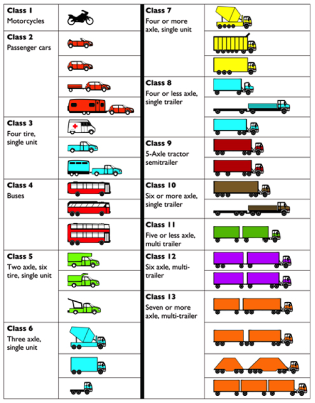
Class 1: Motorcycles
Class 2: Passenger cars
Class 3: Four tire, single unit
Class 4: Buses
Class 5: Two axle, six tire, single unit
Class 6: Three axle, single unit
Class 7: Four or more axle, single unit
Class 8: Four or less axle, single trailer
Class 9: 5-Axle tractor semitrailer
Class 10: Six or more axle, single trailer
Class 11: Five or less axle, multi trailer
Class 12: Six axle, multi-trailler
Class 13: Seven or more axle multi-trailer
Watch This
Watch the first 4 minutes of the Traffic Counting Training Video [103] below which was developed by PennDOT to train traffic count technicians.
Welcome to an overview of PennDOT's traffic counter training. As a traffic field technician, you'll be playing an important role for the Pennsylvania Department of Transportation. PennDOT's traffic monitoring system collects, analyzes, and maintains highway traffic data on over 40,000 miles of roads in Pennsylvania.
Specifically, you will help us collect information on traffic volume and vehicle classification throughout the state. With your assistance, over 10,000 traffic counts are taken annually in Pennsylvania. After all traffic data is collected in the field, it is submitted to PennDOT's central office where it is processed and used to make important decisions about highway design; safety and planning; for research to improve congestion management; to help design and install traffic control systems; to track statistics to help make air quality conformity determinations; to provide information for economic development; and for required federal reporting.
To assist with the collection of this data, traffic field technicians use five types of counting devices. Of these five types, three of them are permanent traffic sites that record information 24 hours a day, 7 days a week, 365 days a year.
The most sophisticated of these permanent devices are Weigh In Motion sensors or WIMs. These sites collect axle weight information as well as vehicle classification information.
The second type of device is the Continuous Automatic Vehicle Classifier or CAVC. These sites collect vehicle classification information.
The third type is the Automatic Traffic Recorder or ATR which collects traffic volume data. The permanent sites have a power source and collect traffic data through magnetic loop sensors, piezos, and/or Kistler sensors that are embedded in the road surface. A modem automatically transfers the data directly to the PennDOT central office daily.
The fourth type of counting device is a semi-permanent counting device commonly referred to as a STIP or Short-Term In Pavement site. The STIP is much like the ATR except that there is no counter in the roadside cabinet. A field technician installs the counter on a predetermined schedule, usually one time a year for a 24-hour period. The counter is then retrieved and the data downloaded and processed.
The fifth type of counting device is a Portable Short-Term Counter. A portable short-term counter installation is a count that is set for a 24-hour period. This type of traffic data collection device provides the majority of the traffic counts taken as part of our statewide count program. A portable short-term traffic counting device collects the data using pneumatic rubber tubing laid across a roadway and attached to a portable counter that has been secured along the side of the road. Tires passing over the road tube register axle counts. The installation of one road tube registers volume counts while a 2 road tube installation produces a vehicle classification count.
The following diagram shows typical setup configurations for portable short-term traffic volume and classification counts: center turn lane class count; center turn lane volume count; divided highway class count; divided highway volume count; two-lane class count; two-lane volume count.
The locations of PennDOT’s permanent traffic counters are presented in a series of district and county maps [104]. Below each map is a table identifying the county, route, segment, and offset of each device. You’ll use this information in Assignment 8-1.
The Value of Traffic Data
Traffic data has a wide variety of uses, a few of the most significant of which are listed here:
HPMS Reporting
One of the most significant uses is to comply with federal HPMS reporting requirements. As was covered last week, states need to report HPMS data to the FHWA each year. HPMS reporting is particularly important to state DOTs since the apportionment of federal funding is based on it.
Highway Safety Improvement Programs (HSIP)
HSIP is a federal aid program aimed at reducing traffic fatalities and major injuries. FHWA requires the project selection process to be data-driven. Traffic data is required to determine crash rates and, consequently, it plays an important role in selecting eligible HSIP projects.
Highway Design
Traffic count data is considered in the design of new roads and the rehabilitation and enhancements of existing roads.
Congestion Management
While real-time congestion management approaches typically use live traffic data based on vehicle speeds, traffic count data can be used to assess congestion and the prospective benefits of ITS technologies.
Roadway Video Logging
Many state DOTs acquire roadway video from specially equipped vehicles which drive all the state-owned roadways. The video data is then made available via a software application which allows users to go on a “virtual drive.” A few examples are Oregon Department of Transportation’s (ODOT) Digital Video Log (DVL) [105] system and PennDOT’s Video Log [106] application. There are many uses of roadway video systems, not the least of which is that they can serve as a means to monitor and maintain roadways and roadway assets, which is both safer and less expensive than an actual visit. The traffic group in PennDOT, for example, uses Video Log to scope out new locations for conducting counts.
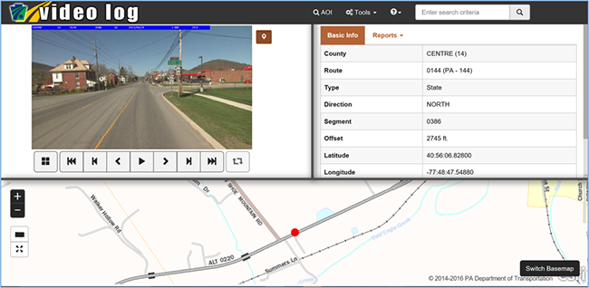
8.2 Getting to Know a Transportation Organization
This week, you’ll take some time getting to know Volpe, The National Transportation Systems Center. Volpe, which is part of the USDOT, is located in Cambridge, Massachusetts and was founded in 1970. It provides a variety of engineering and scientific services to the public and private clients it services and is fully funded by the project work it performs. Its mission is to promote innovative ideas in order to improve the US transportation system. An overview of Volpe’s activities is provided here [107].
Congestion Pricing
Congestion pricing represents a variety of approaches which are aimed at shifting traffic away from a congested section of roadway by implementing pricing surcharges during peak periods to shift some traffic to off times, alternate roadways or alternative modes. In 2007 – 2008, the USDOT invested over a billion dollars to implement congestion-reducing strategies in six US cities. For two of the cities, Volpe was asked to conduct surveys to better understand how congestion pricing affects travel choices. A summary of Volpe’s findings is here [108].
To promote the use of congestion pricing, the FHWA published a primer series on the topic [109], the first of which provided a high-level overview of the concept.
8.3 Getting to Know Each Other
There are no one-on-ones scheduled this week.
8.4 Webinar for Next Week
Speaker
Our speaker will be Mr. Rodney Bunner. Rodney is a Geospatial Technology Specialist who, over the past twenty years, has worked as a consultant to local, regional, state, and federal agencies in developing spatially-enabled and GIS-T applications. He has contributed to the development of a variety of software products and tools within different government sectors including:
- Public Transportation agency support for planning and operations;
- Metropolitan/Regional Planning Organization support for multi-modal transportation planning including travel demand modeling and market assessments;
- State Department of Transportation highway asset management and linear referencing including interactive straight-line diagramming;
- Department of Defense (DOD) facility operations and asset management.
As a public-sector consultant, Rodney’s professional objective has been to develop software applications which streamline the technically challenging and time-consuming data integration, data development, and analytical processes required to fulfill specific government business needs and workflows. To this end, over the past thirteen years, he has been the lead developer for the Florida Department of Transportation’s (FDOT) TBEST Transit Planning software. TBEST provides public transportation agencies with business-specific data, analytics, and reporting tools to address everyday service and strategic planning tasks. Rodney supports numerous agencies throughout the U.S. in implementing and utilizing TBEST.
Rodney is currently the President of ServiceEdge Solutions, a technology company primarily focused on the development of geospatial applications for Transportation. He is a 1991 graduate of West Virginia University with a B.A. in Geography and a 1996 graduate of Shippensburg University of Pennsylvania with a M.S. in Environmental Studies. He currently resides in the Tampa, Florida area with his wife and two children.
Title VI Considerations for Public Transportation Providers
Title VI of the Civil Rights Act of 1964 is intended to ensure people are not discriminated against on the basis of race, color, or national origin in programs which utilize federal funding. Title VI, and the regulations which FTA has put in place to implement it, place specific requirements on transit providers, especially those who provide fixed route services.
Transit Boardings Estimation and Simulation Tool (TBEST)
TBEST is a tool developed by the Florida Department of Transportation (FDOT) to help organizations analyze existing fixed route transit service and potential service changes which are being considered. CUTR has played a big role in the development of the software and also in providing support to agencies who want to use it. A CUTR webinar (57:16) on TBEST can be found here [110]. I provide this link for your reference but watching it is optional. The main speaker in the webinar is Rodney Bunner, next week’s speaker. Consequently, Rodney will likely cover much of the same material in our webinar with him next week. This tool is a very powerful tool and you are able to download and install it for free if you would like. However, you do not need to install it to complete the course requirements.
8.5 Summary of Lesson 8
In this lesson, you learned about the different ways traffic data is collected and used. You also had the opportunity to review PennDOT’s Video Log application and use it to locate some permanent traffic counting devices.
Our transportation organization of the week was Volpe, The National Transportation Systems Center. You learned about some of the initiatives in which Volpe is engaged. In particular, you explored the concept of congestion pricing and reviewed some applications of these strategies including the manner in which they affect driver behavior and their overall effectiveness in mitigating congestion.
In our weekly webinar, you had the chance to interact with two transportation professionals. Mr. Jeff Roecker spoke about some of the tools and approaches PennDOT uses to improve highway safety and Mr. Jeremy Freeland spoke about HPMS reporting and the roles that spatial tools play in the implementation of a statewide traffic count program.
Finally, in preparation for next week’s webinar, you learned about a transit planning tool called TBEST and you reviewed some requirements that transit agencies need to meet which are based on Title VI of the Civil Rights Act of 1964.
Questions and Comments
If there is anything in the Lesson 8 materials about which you would like to ask a question or provide a comment, submit a posting to the Lesson 8 Questions and Comments discussion. Also, review others’ postings to this discussion and respond if you have something to offer or if you are able to help.
Lesson 9: Transit
Learning Outcomes
What will we learn?
By the end of Lesson 9, you should be able to:
- describe the nature of DRT services and the primary populations they are intended to serve;
- list some of the technologies providers use to help them manage DRT services;
- characterize the most common types of DRT fare structures;
- discuss some of the characteristics of fixed route transit and explain the structure and function of GTFS data;
- describe some of the functions and accomplishments of the Federal Transit Administration (FTA);
- share something you learned about one of your classmates and/or some ideas you discussed with a classmate about the content of this week’s lesson.
9.1 Transit
Transit organizations typically offer two distinctly different types of service: Demand Responsive Transportation (DRT) and fixed route transportation. Fixed route transportation operates according to prescribed routes and schedules whereas DRT does not. In this lesson, we will look at both of these types of transit.
Demand Responsive Transportation (DRT)
DRT is generally designed to provide curb to curb or door to door service for individuals who have special transportation needs such as seniors and persons with disabilities. The availability of DRT services can vary significantly from state to state and even county to county based on funding availability. DRT differs from taxi service in two fundamental ways:
- To use DRT, a rider must make an advance reservation (generally, at least 24 hours in advance).
- DRT is a shared-ride type service where multiple riders can be serviced at the same time, and a rider is generally not taken directly from their point of origin to their point of destination. Consequently, DRT trips can have substantially longer ride time than taxi trips.
DRT services are generally designed to serve rural areas where fixed route transit is not practical due to low ridership and also to complement fixed route services for those who live near a fixed route but are unable to use it due to physical or cognitive limitations.
ADA Complementary Paratransit
The Americans with Disabilities Act (ADA) of 1990 prohibits discrimination against persons with disabilities in a number of areas including public transportation. The FTA has defined a series of requirements public transit providers need to meet to comply with the ADA. These requirements are found in Title 49 Part 37 of the Code of Federal Regulations (CFR). In these regulations, the FTA requires fixed route providers to provide DRT service, comparable to the level of service provided to individuals who are able to utilize fixed route services, to persons with disabilities. DRT services designed to address the needs of persons with disabilities is known as paratransit service. Specifically, bus or rail fixed route providers are required to offer paratransit services to individuals who are unable to use the fixed route service due to physical and/or cognitive limitations, who live within ¾ of a mile of a fixed route and are traveling to a destination which is also within ¾ of a mile of a fixed route. This requirement is challenging and costly for transit providers to fulfill. It applies to all providers, and not just those who are receiving federal funding. It is also an unfunded mandate in that FTA does not provide grant monies to transit agencies to help offset the cost of compliance. You’ll complete an assignment next week to evaluate the eligibility of a series of trips for complementary paratransit service.
Technologies for DRT Services
Providing DRT services in a way which is both cost effective and customer friendly is a very challenging task. The number of riders requesting service can vary substantially from day to day as can the trip origins and destinations. Service requests are initiated by riders through a call to a Customer Service Representative (CSR). Reservations typically need to be made at least 24 hours before service. Generally, the day before services are delivered, schedulers need to determine how to accommodate all of the reservations for the day with a limited number of vehicles and drivers. Further, the schedulers need to ensure a wide variety of constraints are met, including promised pickup time, required drop off times (e.g., for medical appointments) and total ride time. On the day of service, dispatchers work with the drivers to ensure all trips are successfully completed. Drivers follow a trip manifest which defines which stops they will visit and the order in which they will visit them. Drivers also need to track a variety of data elements at each stop including arrival and departure times, the passengers boarding and alighting at each stop, the vehicle odometer reading, and the amount of money collected from each passenger.
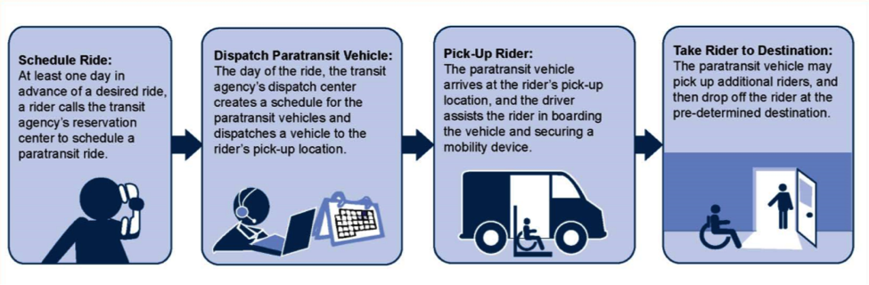
For all but the smallest providers, it would be very difficult to manage DRT service without technology. The most important technology which providers use is DRT software. Most DRT software assists the providers with all of the key tasks associated with delivering and reporting on the service. Many systems incorporate Automatic Vehicle Location (AVL) technology, which allows the dispatcher to monitor the location of all of their vehicles. This can be extremely useful in terms of ensuring drivers stay on task and follow the manifest. Some of the more sophisticated packages can do automated scheduling. These systems determine the best vehicle for a given trip reservation. DRT scheduling is very complex, owing to the large number of variables involved, many of which are related to human behavior, and as a result, even software that can do automated scheduling cannot produce good schedules without significant scheduler oversight.
Interactive Voice Response (IVR) technology is also playing an increasingly important role in DRT operations. Typically, systems which incorporate IVR will configure the system to automatically call riders the night before a scheduled trip to remind them of the trip and give them an opportunity to cancel the trip. Systems will also generally automatically call the riders when the vehicle is approaching their location. These calls, known as imminent arrival calls, are valuable for both the provider and riders. Providers benefit because the calls ensure riders will be ready, and riders benefit since the calls give them a clear idea of when to be ready and eliminate the need for them to wait outside for a prolonged period. IVR plays a significant role in reducing “No-Shows” where the driver gets to a location to pick up a rider and the rider is not there. No-shows add additional costs to a service which is already expensive to provide.
Many providers give their drivers Mobile Digital Computers (MDC) which serve a variety of functions. More and more DRT software vendors are shifting to tablet technology instead of using proprietary hardware. MDCs provide additional communications with dispatch via canned or ad hoc text messages. The MDCs also generally present the trip manifest information to the driver in an electronic form and tell the driver their next stop location, how well they are adhering to the schedule, how many passengers should be boarding and alighting at each stop, and how much money they should collect from each person. The driver also uses the MDC to capture the information they need to collect such as the stop arrival time, the passengers who boarded and who alighted the vehicle at the stop, how much they collected from each rider, and what time they departed from the stop. MDCs can also be configured to provide the driver with turn-by-turn directions and eliminate the need for a separate GPS device.
Fare Structures
Transit agencies use a number of different methodologies to establish a fare structure for their DRT services. The three most common are listed below:
Flat – In a flat fare structure, as the name implies, the cost of the trip is the same regardless of origin and destination, assuming both are within the agency’s service area.
Zone-Based – In a zone-based fare structure, the agency divides its service area into zones. The zones are generally comprised of a series of concentric circles or a rectangular grid which blankets the service area. Fares are then established for each origin and destination zone.
Mileage-Based – In a mileage-based fare structure, the agency develops a series of mileage-based tiers and associates a fare with each. The mileage associated with each trip depends only on the origin and destination and not on other pickups or drop-offs the driver may have performed while the passenger is in the vehicle. Consider the following example:
Ellen makes a reservation to go to the senior center on Monday at 10 am. On Friday afternoon, the agency’s scheduler is working with their paratransit software to finalize the driver manifests (i.e., schedules) for Monday morning. This process involves determining the most efficient way to deliver the service while at the same time observing customer service policies such as ensuring all riders get to their appointments on time and do not exceed the maximum onboard time established by the agency. On Monday morning, the drivers depart the transit agency and begin to execute the manifests (i.e., schedules) that have been prepared for them. The driver assigned to pick up Ellen arrives at her house to pick her up at 8:45 am. The driver then drives to Allen’s house to pick him up and on to Sue’s house to pick her up. He then drives to the VA hospital to drop off Allen and to Walmart to drop off Sue. Finally, he drives to the senior center and drops Ellen off at 9:50 am.
The driver may have visited many stops while Ellen was on the vehicle, but the mileage used for fare determination is based only on the route from her origin to her destination. When an agency uses a mileage-based fare structure, they can base the mileage on the fastest route from the origin to destination or the shortest distance route from the origin to destination.
9.2 Fixed Route Transit
Fixed route transit services can be defined as services which operate on predefined routes according to a set schedule. The services can be divided into a number of more specific modes including:
- Local Bus
- Commuter Bus
- Express Bus
- Bus Rapid Transit
- Light Rail
- Subway
- Ferry Boat
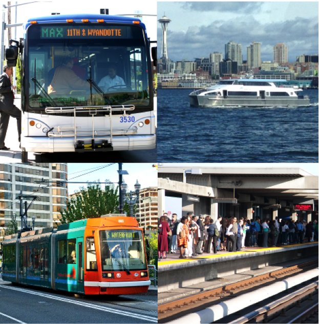
Routes and Patterns
Fixed route buses operate on designated routes according to a published schedule. One can think of routes as generalized paths buses follow. For example, Route 1 may be structured to provide service along Market Street. It may begin at a transit center where riders can transfer from one route to another or even to a different mode such as light rail or subway and travel along Market Street until it reaches some terminal point at which time it returns along Market Street to the transit center. The specific path each route traverses can depend on the time of the day, the day of the week, and even the time of year (e.g., summer service). Each distinct path associated with a route is called a pattern. As an example, Figure 9.2 and Figure 9.3 show two patterns for the same route. The route generally follows Pattern 1, but at times during the day when the YMCA is busiest, it follows a somewhat different pattern.
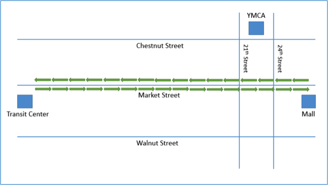
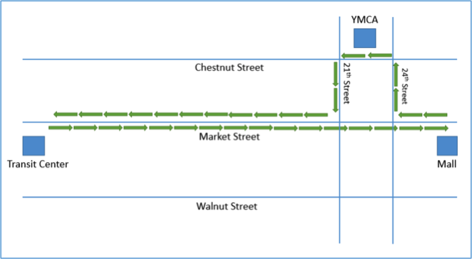
Trips, Headway, Interlining, and Vehicle Blocks
When one uses the term trip in regards to DRT, it generally refers to the transport of a rider from their point of origin to their desired destination. In fixed route, the term trip has a different meaning. Over the course of a day, service along a route will generally be offered a number of times. For example, service along Market Street, in the above example, may occur at a frequency of twice an hour from 9 am to 4:30 pm, with a bus leaving the transit center every 30 minutes. In the world of fixed route, a trip corresponds to a bus completely traversing the route one time. The period of time between each trip is called the headway. In this example then, there are 16 trips and the headway is 30 minutes. If it takes more than 30 minutes to complete a single trip, then it will take multiple buses to provide service along Market Street. Sometimes a bus will operate a single route the entire day, and sometimes a bus will service multiple routes. When a bus completes a trip on one route and then begins a trip on a second route, it is referred to as interlining. A bus's schedule for an entire day is called a block. For example, Bus 2a may operate on Route 1 from 9 am to 12:30 pm, at which time it is used on Route 2 from 1 pm to 5 pm. The block for Bus 2a would be the sequential set of trips it completes over the course of the day on Routes 1 and 2.
Stops, Time Points, and On-Time Performance
A stop is a designated location along a route where riders can get on or get off the bus. The bus is obligated to stop at certain stops known as time points. These are stops that appear on the bus schedule. Generally, a transit agency will have a policy that a bus should not depart a time point before the scheduled time. How well a transit provider adheres to its published schedule is referred to as its on-time performance. It is important for transit providers to adhere to their schedules since riders depend on transit to get to their destinations on time. There are also stops along a route which are not time points. The bus will only stop at these stops if a rider is waiting at the stop or if a rider wishes to alight the vehicle at the stop. In addition to defined stops, some providers accommodate flag stops. A flag stop is an arbitrary location along the route where a rider wishes to board or alight the bus. The rider needs to flag the bus down in order to board or alert the driver they wish to alight the bus at that location.
Runs and Run Cutting
Sometimes, a single driver will operate on the same bus and route all day long. At others times, the driver may operate on a number of buses and/or routes over the course of the day. The collection of trips a driver performs over the course of their shift is known as a run. Just as a block represents a bus's schedule for the day, a run represents the driver's schedule for the day. Matching drivers with the pieces of work a transit provider needs to staff is known as run cutting. Run cutting can be a complex process at least in part because drivers and other staff often belong to a union, and the labor agreements which have been negotiated can have many different rules which need to be followed.
Fixed Route Technologies
Fixed route providers use a large number of technologies to manage operations and provide good customer service. The most significant of these technologies are described briefly below:
Fare Collection
There are a variety of fare collection technologies which fixed route providers use to collect and securely store fares. Some fare boxes are able to assist the driver in verifying that cash-paying riders provided the correct fare. Registering fare boxes are able to count coins and bills, but they cannot differentiate between different denominations of bills. For example, a registering farebox can’t tell the difference between a one dollar bill and a twenty dollar bill. Validating fare boxes can do everything a registering fare box can do and, in addition, can differentiate between different denominations of bills. Registering and validating fareboxes also generally allow the drivers to keep track of the types of passengers who are boarding (e.g., seniors, persons with disabilities, children, etc.). For providers who have relatively low ridership, it is difficult to justify the cost of registering or validating fare boxes. For these types of providers, a vault style fare box is often the most logical choice. A vault style fare box does not count cash payments. Instead, the upper compartment is generally transparent which allows the driver to confirm the correct fare was provided before it is dropped into the lower compartment. Many providers are moving toward providing more flexible payment options. Touch cards are a convenient type of fare media which are growing in popularity. Riders can generally add additional value to these cards using a ticketing machine or via the web.
Computer Aided Dispatch / Automatic Vehicle Location (CAD/AVL)
Many transit organizations who operate a fixed route bus service use CAD/AVL. CAD/AVL systems consist of onboard hardware to track the buses, and software which helps the dispatchers to manage service as it is occurring and resolve issues as they arise. CAD/AVL allows the dispatcher to see where all the agency's vehicles are on a map and to quickly determine which are on schedule and which are ahead of schedule or behind schedule.
Automatic Passenger Counters (APC)
APCs are simple devices which are mounted by each door and count the number of passengers boarding and alighting the bus. While there are different types of APCs on the market, the most common employ a series of infrared beams. Each time the beams are broken, the system counts it as either a boarding or alighting. During busy times, the devices can miss a passenger here and there. The devices can also have a hard time with children, especially if they are carried onto the bus. The data collected via APCs can be used to determine the current onboard passenger count, a piece of information that is sometimes made available to the riding public along with other real-time bus information. Transit agencies sometimes also use APC data to fulfill part of their reporting NTD requirements to the FTA but, in order to do so, they need to demonstrate that their APCs meet certain accuracy requirements. You'll learn about NTD reporting later in this lesson.
Automated Announcement Systems (AAS)
In order to comply with ADA requirements, fixed route vehicles are generally equipped with an AAS which provides both audible announcements and visual announcements about upcoming stops and points of interest. These systems are generally triggered based on the vehicle's position as it approaches a designated location. Most systems utilize geofences to determine when an onboard announcement should be made.
Vehicle Surveillance
Most fixed route vehicles are equipped with camera systems which record activities on the bus as well as outside the bus. It is common for a bus to have 6 separate audio and video streams with some of the larger articulated buses being equipped with 8 separate streams. The video from these buses is stored in onboard DVRs and can be streamed by dispatch if needed. The DVR capacities are generally sufficient to store a few weeks of video before overwriting. The systems are configured to automatically flag sections of video in the event the system senses any unusual forces due to a collision or abrupt deceleration or turn. The driver can also press a button to manually flag a section of the video. When the system flags a section of the video, it preserves a window of time which brackets the triggering event for later review. Flagged sections of video are often wirelessly downloaded when the bus returns to the depot. Vehicle surveillance systems are extremely useful for identifying undesirable driver behaviors and incidents onboard the bus, as well as helping to determine the cause of any bus-related accidents. Local police are also sometimes interested in this video if they believe it may be of use in solving or prosecuting a case.
Real Time Passenger Information
Real time passenger information systems have become extremely popular in recent years. These systems make real-time bus information available to riders via web applications, smartphone applications, and dynamic message boards which are sometimes located as transit centers or other high traffic stops. In Lessons 8 and 9, we looked at an example of one which CATA uses called MyStop.
Rider Alerts
Transit providers often offer rider alert systems to notify users about disruptions in services or to provide other types of notifications. Riders can typically sign up for alerts related to specific routes and/or system-wide alerts.
Scheduling Software
Developing and adjusting routes, patterns, stops, trips, and blocks can be challenging especially for larger transit providers. Scheduling software is designed to assist agencies in this regard. Scheduling software also often incorporates some functions to assist with run cutting as well.
Vehicle Health Monitoring
Many buses come equipped with vehicle diagnostics that can transmit various vehicle health information back to the transit agency. This technology helps to ensure problems are taken care of before they lead to vehicle breakdown. Some vehicle health systems integrate with maintenance management systems and can automatically schedule vehicles for preventative maintenance.
Trip Planning/Google Transit
Many fixed route providers offer trip planning services to their riders. These services are generally web-based and allow the rider to indicate their origin, destination, and desired date and time of departure or date and time of arrival. The trip planning service then presents options which define a combination of walking and fixed route options that best meet their needs. The options may involve one or more transfers between fixed route vehicles. The most popular fixed route trip planning service is Google Transit. The idea for what has become Google Transit was first spawned by TriMet, a transit agency which services Portland, Oregon. TriMet approached MapQuest, Yahoo, and Google to see if they would be interested in incorporating transit data into their map products, but only Google replied. The Google Transit Trip Planner launched on December 7, 2005. Google transit incorporates stops, routes, schedule, and fare information for a provider’s bus, subway, rail, and/or light rail service. The service is automatically available as a free service via Google Maps in any area where one or more local transit providers publish their data to Google.
For most of the first year, TriMet was the only operator available on Google Maps. In September 2006, five more cities got on board: Eugene, OR; Honolulu, HI; Pittsburgh, PA; Seattle, WA; and Tampa, FL. Today, Google Transit spans many hundreds of cities [111].
In order for transit providers to submit their fixed route information to Google in a consistent way, a data specification was required. The specification which was developed for this purpose is discussed in the next section. As mentioned above, Google Transit is a free service to transit agencies and to the public who can perform trip planning in Google Maps. However, if you wish to tie into the capabilities programmatically to incorporate the power of Google Transit (or more generally Google Maps) into your own software application, there are often associated fees you need to consider. A popular and robust alternative open source trip planning system is Open Trip Planner [112].
General Transit Feed Specification (GTFS)
The specification which was developed to allow transit agencies to publish their fixed route data to Google Transit is known as GTFS. Originally it stood for the Google Transit Feed Specification, but in 2010, Google changed the name to the General Transit Feed Specification given its growing status as the default specification for transit data. GTFS is an open data standard which represents fixed-route schedule, route, and bus stop data in a series of 13 comma-delimited text files compressed into a ZIP file. Each of the 13 text files contains a series of fields or attributes about a component of the fixed route service. Some of the files and fields are optional (see Table 1).
| Required | Optional |
|---|---|
| Agency.txt | Calendar_dates.txt |
| Stops.txt | Fare_attributes.txt |
| Routes.txt | Fare_rules.txt |
| Trips.txt | Shapes.txt |
| Stop_times.txt | Frequencies.txt |
| Calendar.txt | Transfers.txt |
| Feed_info.txt |
Click for description of each table [113] along with the meaning of each field.
The primary use of GTFS data is to publish fixed route schedule data to Google Transit so that riders can perform trip planning. However, there are many other potential uses for GTFS data. For example, transit planning software systems such as TBEST commonly allow users to upload route, stop, and schedule data in GTFS format. In the past few years, Google has created a new specification based on GTFS which incorporates real-time information in addition to the static schedule data. The new specification is known as GTFS Real Time [114] and is starting to gain some traction among transit agencies, but is not yet widely used.
In Assignment 9-2 you’ll have a chance to work with GTFS data from a transit agency in Tampa, Florida. Specifically, you’ll use the route geometry contained in the shapes.txt component of the GTFS data to establish the zone for ADA complementary paratransit.
The following assignment is optional. You do not need to complete this assignment to fulfill the requirements of the course. TBEST is a powerful tool for transit planning and is available for free. If you have an interest in the tool, this assignment will help you to get some hands-on experience using it.
Optional Assignment
In this assignment, you’ll get a chance to get some hands-on experience with TBEST as you explore some of its many features. Prior to doing this assignment, you will need to download and install TBEST Version 4.4 for ArcGIS 10.5. As part of Assignment 8.6, you reviewed some tutorial videos which are available to help users learn how to use the features TBEST offers. In preparation for this assignment, watch the tutorial videos on scenarios, network tools, TBEST reporting, and the attribute search tool. TBEST also has a comprehensive users' guide [115]available from both the website and the help menu within TBEST. Complete the following activities.
- Open TBEST.
- Download Socio-Economic data, GTFS Data, and a transit system logo.
- Under the File menu, select “Downloads”, select “Download Socio-Economic Support Data...”, and finally select “Florida 2014 Population 2014 Employment 2015 Parcel”, and click “Download”.
- Download the latest GTFS file [116]for HART.
- Download the transit system logo [117]for HART.
- Create a new transit system.
- For this assignment, you’ll model Hillsborough Area Regional Transit (HART) which services Tampa in Hillsborough County.
- In the TBEST explorer window, right click “Transit Systems” and select “New System”.
- You will be prompted to select the source socioeconomic data. The only option you have is the data you downloaded in step 2. Select it and click “Ok”.
- On the “New Transit System” dialog, enter HART as the transit system name.
- Select Hillsborough County as the extent.
- Leave the remaining settings alone and click “Ok”.
- It will likely take 60-90 minutes to compile the socioeconomic data and parcel data for Hillsborough County, Florida.
- Create a new TBEST Scenario.
- In the TBEST explorer window, expand the HART transit system you created in step 5.
- Right click “Scenarios,” and select “Create a New Scenario…”
- Name the new scenario “2017 Base Conditions”.
- Select “TBEST Land Use Model 2016” as the scenario model (it is the only option).
- Enter “2017” as the Forecast Year.
- Select an average annual wage for Hillsborough County and enter it as the mean annual wage for the scenario.
- Enter “2” as the annual growth rate.
- Click “Ok” to create the new scenario.
- Create HART’s Fixed Route Network.
- You’ll create HART’s fixed route network by importing their latest GTFS data file. As an alternative, you could manually create the network in TBEST, but that would be time-consuming.
- In the TBEST explorer window, right click on the “2017 Base Conditions” scenario and select “Import Routes from GTFS”.
- On the TBEST GTFS Network Import dialog, select the GTFS.zip file downloaded in step 2b as the source GTFS zip file.
- Select the top three checkboxes (i.e., Weekday, Saturday, and Sunday) to select all service periods.
- Click “Load Routes” to load all routes.
- Check “Select All” in the lower left corner of the dialog to select all routes.
- Click the “Import” button to begin importing the network.
- You will be prompted for confirmations 2 times. Click “Ok” to both.
- Once the network has been successfully imported (it should take about 10 minutes), you can exit the GTFS Network Import screen.
- Exploring HART’s Fixed Route Network.
- Right mouse click on the newly created “2017 Base Conditions” scenario and select “Open Scenario”.
- Grab a screenshot of the resulting map showing HART’s routes. (5 points)
- In the routes window, expand Route 1 – Florida Avenue.
- Expand the Northbound Patterns.
- Double click Pattern 40317.
- TBEST automatically highlights the pattern and associated stops on the map.
- In addition, the segments and stops are automatically populated in their respective windows.
- Grab a screenshot of the entire TBEST window with Pattern 40317 selected. (2 points)
- TBEST has powerful search capabilities which allow you to find and select a group of stops, segments, or routes based on attribute filters. The search tool is available on the main TBEST toolbar (binoculars) or via the Scenario menu.
- Open the search tool and search for stops associated with express routes.
- To do so, select “Stops” as the Category, “Route Type” as the attribute, “Equal To” as the Operator (i.e., “Is”), and “Express” as the Value.
- Click “Add to Search Criteria” to add the filter.
- Click “Apply” perform the search.
- Grab a screenshot of the map showing the express route stops selected. (3 points)
- Group selecting routes, segments, and stops in this manner is useful for mass adjusting attributes for alternative scenario modeling. For example, you could use the stop calculator to adjust the headway of all currently selected stops to 20% less than each stop’s current headway setting.
- Set Socio-Economic Growth Rates and Base Fares.
- Under the Scenario menu, select the “Set Socio-Economic Growth” submenu, and finally “Enter Growth Rates”, to bring up the “Socio-Economic Data Growth Rates” dialog.
- Enter 2% in total population. By default, this rate will be used for the other factors as well.
- Click “Set Growth Rates” to apply the rates and close the dialog.
- To establish the base fares, open the System Fare Levels Dialog ($ Icon on the main TBEST toolbar, or select “System Level Fares” from the “Scenario” menu).
- Base fares are set according to the route type. All of HART routes are of one of three types: Circular, Radial, and Express.
- In the dialog enter $6 for the express routes and $4 for the circulator and radial routes.
- Click “Ok” to apply the fares and close the dialog.
- Running the Model.
- You are now ready to run the model. To do so, right-click the “2017 Base Conditions” scenario in the TBEST explorer window and select “Execute Model Run”.
- On the “Scenario Model Run” dialog, you will use the default settings and click “Run”.
- You will be asked to confirm the run and whether you want to save changes to the scenario. Click “Yes” to both.
- It will take about 20 minutes to run the model.
- Examining Model Results.
- On the “Scenario” menu, select “Model Reports” and then “Scenario Summary Tool”.
- Select the HART transit system and the “2017 Base Conditions” scenario.
- Leave the default “Summary Span and Time Period” settings as is, and click “Show Report”.
- Explore the results presented here.
- Examine the performance measures “Boardings Per Service Hour” and “Boardings Per Stop Visit”.
- Which route has the highest “Boardings Per Service Hour”? (2 points)
- Generate a chart showing these 2 performance measures for the HART express routes and a handful of the non-express routes (Hint: You can use the TBEST search tool to identify express routes).
- Examine how the relationship between these 2 performance measures in general differs between express routes and other routes (e.g., “Boardings Per Service Hour” are high and “Boardings Per Stop Visit” are low).
- Grab a screenshot of the chart. Identify the routes which are express routes. Describe any difference in relationship you observe. How might you account for your observations? (3 points)
- Title VI Analysis
- To run a Title VI Analysis, you need to have all scenarios closed. You can close any open scenarios by clicking “Close Scenario” on the main TBEST toolbar.
- Right mouse click on Title VI Analysis in the TBEST explorer window and select “New Title VI Analysis”.
- Name the new analysis “Route 1 Title VI Analysis”.
- Select “HART” as the transit system.
- Select “2017 Base Conditions” as the scenario.
- Leave the buffer distance as 0.25 miles and click “Next”.
- Leave the service area setting as Hillsborough County and click “Next”.
- On the Poverty Levels screen, adjust the poverty incomes to reflect the 2017 values [118]from the Department of Health and Human Services and, once done, click “Next”.
- On the “Route Selection” screen select Route 1 and click “Next”. (Note: we are running just 1 route for this exercise, so the analysis will complete faster.)
- Upload the transit system logo for HART and click “Next”.
- Click “Next” on the “Jurisdictional and Rex Route Input” screen.
- The Major Roads screen already has the correct shapefile selected. For states other than Florida, you would need to download the correct TIGER road data. Click “Next”.
- Click “Finish” on the “Title VI Setup Screen”.
- Click “Yes” on the confirmation screen.
- After a few minutes, the Title VI Analysis will finish, and the “Title VI Analysis Console” appears. On the left side of the console, there is a variety of maps, and on the right side, there are a series of reports. Maps open in ArcMap.
- Spend a few minutes exploring the variety of output. Grab a screenshot of 1 map and 1 report you find interesting and briefly describe each. (5 points)
9.3 Getting to Know a Transportation Organization
This week, you’ll take some time to get to know the Federal Transit Administration (FTA). The FTA is the administration within the USDOT which focuses on providing financial and technical support to public transportation agencies across the United States. The FTA was created in 1970 by President Lyndon Johnson, although, back then, it was known as the Urban Mass Transportation Administration (UMTA).
This short video (12:45) summarizes some of FTA’s accomplishments over the past 8 years and provides examples of how it has directed federal funds.
ON SCREEN TEXT: Together a look back at the last 8 years. (Countdown begins:) 2016, 2015, 2014, 2013, 2012, 2011, 2010, 2009, 2008. With growing congestion...[TRAFFIC NOISES] and aging infrastructure [CREAKING BRIDGE]...with an economy in freefall [IMAGES OF NEWSPAPER HEADLINES ON FINANCIAL CRISIS]
January 20, 2009. "Starting today, we must pick ourselves up, dust ourselves off, and begin again the work of remaking America." [IMAGES OF FORMER PRESIDENT OBAMA'S INAUGURATION}
BARACK OBAMA: For everywhere we look, there is work to be done. The state of our economy calls for action, bold and swift, and we will act -- not only to create new jobs, but to lay a new foundation for growth. We will build the roads and bridges, the electric grids and digital lines that feed our commerce and bind us together.
ON SCREEN TEXT: Together we answered the call. To meet growing demand, to replace again infrastructure, to get our economy moving again, President Obama and Congress acted.
BARACK OBAMA: Building a world-class transportation system is part of what made us a economic superpower. There are private construction companies all across America just waiting to get to work. There's a bridge that needs repair between Ohio and Kentucky that's on one of the busiest trucking routes in North America. Public transit project in Houston that will help to clear up one of the worst areas of traffic in the country.
ON SCREEN TEXT: The American Reinvestment and Recovery Act (ARRA). Over the next four years, USDOT awarded 1,072 ARRA grants totaling $8.8 billion, creating or saving 10,322 jobs. Transportation Investment Generating Economic Recovery (TIGER) grants: Also, in 2009, Congress passed legislation establishing the TIGER program. TIGER grants have provided $5.1 billion to 421 projects, helping build multi-modal, road, rail, transit, and port projects and rebuilding communities.
Dilworth Plaza, Philadelphia, PA. A $15 million TIGER grant transformed a deteriorated plaza at City Hall and helped create a new, accessible gateway for local and regional transit.
Kansas City, MO Streetcar. A $20 million TIGER grant helped generate $1 billion investment in KC's downtown. Kansas City Streetcar opening, May 2016.
East Liberty Transit Center, a $15 million TIGER grant renovated an aging bus station and consolidated unsafe loading points along Pittsburgh streets. East Liberty Transit Center, Pittsburgh, PA, October 2015.
Denver Union Station, a $388 million TIGER grant helped renovate a station that anchors a bustling downtown and spun off new development. Denver Union Station Renovation March 2014.
LYNX Lymmo BRT, a $13 million TIGER grant enabled this new line, which connects to other transit modes and revitalizes Orlando's urban core. LYNX Lymmo BRT Groundbreaking, Orlando May 2015.
In 2010, transit ridership reached 10 billion, its highest level since the 1950s.
Capital Investment Grants: new starts, small starts, core capacity. Since 2008, FTA has funded 37 Capital Investment Grant projects totaling $12.6 billion. Since 2008, CIG projects have resulted in 296 miles of rail & 158 miles of Bus Rapid Transit.
Other FTA grant programs. Since 2010, FTA has awarded close to $3 billion to 601 competitively funded bus projects. That funding led to the purchase of more than 53,000 buses since 2009. FTA has also funded the purchase of over 27,000 other transit vehicles, such as paratransit vans: GO Transit- Durham, NC, Capital Metro - Austin, TX, Niagara Frontier - Buffalo, NY, KCATA - Kansas City, MO, CATS - Charlotte, NC, Free Ride Transit - Breckenridge, CO.
Since 2009, FTA has awarded close to $286 million for tribal transit: Los Alamos, NM, Muscogee Creek Nation, Mississippi Band of Choctaw Indians.
Since 2013, FTA has funded 44 Passenger Ferry grants totaling $119 million: Channel Cat - Quad Cities, Iowa, Staten Island Ferry, NYC DOT, Kind County Ferry - Sound Transit. But America requirements have contributed to a strong U.S. manufacturing sector and supported American jobs. Together we helped rebuild our economy, meet growing demand for transit, and begin to fix our aging infrastructure. Together we faced emerging challenges. Together we're making the transit, the safest form of transportation, safer. MAP-21 and the FAST Act gave FTA new and enhanced authority to help keep public transit safe and reliable. Since 2012, with your input, FTA has issued: 3 final safety rules, 3 proposed safety rules, 7 safety advisories, and is working to strengthen state safety oversight.
Natural Disasters and Climate Change. In 2012, Hurricane Sandy struck the East Coast. Since 2013, FTA has awarded $10.2 billion in grants focused on Sandy recovery and resiliency. Extreme weather events highlight the dangers of climate change. Together, FTA and our transit partners are developing strategies to prepare for and adapt to climate change.
The transportation industry as a whole is a major contributor of carbon pollution, but public transportation can help. FTA's Low and No-Emission Program aims to improve air quality and reduce climate change through new bus technology. Since 2012, FTA has funded 37 Low - and No-Emission Grants totaling $132.5 million.
Declining Infrastructure. In 2013, the transit industry's deferred maintenance and replacement needs was estimated at $86 billion and it keeps growing. Transit Asset Management Final Rule July 2016. TAM provides a strategic approach to improve & maintain transit capital assets and requires providers to create plans to address their maintenance needs.
"When the rungs on the ladder of opportunity grow farther and farther apart, it undermines the very essence of America" - President Obama
"Transportation is about more than getting from on point to another, it's about getting from where you are to a better life." - Transportation Secretary Anthony Foxx
As part of DOT's Ladders of Opportunity bus program, DOT awarded $26 million to Detroit. The city bought 50 buses easing overcrowding, reducing wait times, and providing more reliable service, particularly in lower income areas. Together we've built ladders of opportunity.
Since passage of the Americans with Disabilities Act in 1990, transit has become more accessible. Thanks to transit providers, 99.8% of buses are accessible. All rail stations built since 1990 are accessible. In addition, 671 of 680 key stations in our nation's oldest rail systems are accessible.
Since 2012, FTA has issued three civil rights Circulars helping the industry provide more equitable service.
Since 2013, FTA has funded 21 Transit-Oriented Development Grants totaling $19 million. Together, we're using well-planned TOD to create more desirable places to live, work, and visit.
FTA's Rides to Wellness initiative improves access and reduces healthcare costs through partnerships between health care and transit industries. New in 2016, Rides to Wellness Grants awarded $7.3 million to 19 projects.
Together we've helped communities across the country:
- Twin Cities Central Corridor Light Rail; $474 million CIG funding.
- Pocatello Regional Transit Center; Bannock County, Idaho; $1.4 million Bus Grant
- Metrolink Commuter Rail, Perris Valley, CA; $75 million CIG funding
- Dallas Area Rapid Transit's 24-mile Green Line Light Rail; $700 million CIG funding
- Austin Metro Rapid BRT; $38 million CIG funding
- SunRail Commuter Rail, Central Florida; $93.4 million CIG funding
- Utah TRAX Light Rail, Salt Lake City; $460 million CIG/ARRA funding
- LA Metro Rail System, $4.1 million CIG funding
- CT FasTrak, Hartford, Connecticut; $275 million CIG funding
- VelociRFTA BRT, Roaring Fork Valley, Colorado; $25 million CIG funding
- TriMet Orange Line light rail extension/Tilikum Crossing, Portland, Oregon; $745 million CIG funding
Together, we are embracing the future. The FAST Act was the first long-term infrastructure funding bill since 2005. While it provides certainty for transit systems, we still need a stable funding source for the future. Technological innovation is bringing us the chance to solve old problems in new ways. FTA's Mobility on Demand program will provide $8 million for innovative integrated multimodal solutions.
At FTA, we're proud of all that we've accomplished...Together:
- State Safety Workshop, July 2016
- Birmingham, AL TIGER announcement September 2015
- ADA Event, Washington, DC August 2015
- Metrolink Commuter Rail Extension, December 2016
- Denver Light Rail to DIA Opening, April 2016
- WMATA New Rail Car Announcement May 2015
- SEPTA Wayne Junction Commuter Rail Opening, April 2015
- Veterans Transportation and Community Living Initiative Grant Announcement, Albuquerque, NM
- Cleveland Cedar-University Rapid Station Opening, August 2015
- El Paso Northgate Transfer Center Opening, September 2013
- Jacksonville, FL First Coast Flyer BRT Groundbreaking, November 2014
- Bethesda, MD ADA Event August 2015
9.4 Getting to Know Each Other
This week, you’ll have a one-on-one chat with one of your classmates as per the schedule you were provided in Week 1. The discussion should be at least 30 minutes in length. If it’s the first time you’ve chatted with each other, spend the majority of time getting to know each other. Otherwise, focus on discussing the lesson content.
9.5 Webinar for Next Week
Public transit organizations provide important services which alleviate congestion and which offer mobility to those who have no other transportation options. While they all have some common objectives and challenges, transit organizations are each unique, based largely on differences in the communities they serve and in the political landscape they operate under at both the state and local level. Next week, we'll hear from 2 speakers who represent two separate transit organizations.
Speaker #1
Our first speaker will be Dr. Minhua Wang. Dr. Wang has over 25 years' experience in IT and GIS, has served multiple positions in government agencies, software development companies, and consulting firms. Dr. Wang has developed expertise and reputations in the areas of GIS for transportation or (GIS-T), Public Transit, and transportation software development and implementation. His experiences in the transportation GIS field include data modeling, enterprise architecture design, system integration, application development, asset management, and GIS technology implementation. Dr. Wang currently serves as GIS Manager in the Washington Metropolitan Area Transit Authority (WMATA). He has overall responsibility for administrative, technical and managerial tasks necessary for the development and operation of Metro’s enterprise Geographic Information System. He has involved considerable interaction, cooperation and collaboration with managers throughout Metro, and officials of other public agencies and regional partners in the design, development, and implementation of the geographic information system and related products to meet various needs and functions. Prior to WMATA, Dr. Wang served as Project Manager at DC Department of Transportation (DDOT), Group Leader at CitiLabs (a Transportation Planning Software company), Enterprise Architect at KCI Technology Inc., and Technical Architect/Director of Application Development at Geodecisions. Dr. Wang holds a Ph.D. degree in GIS from the University of Waterloo, Canada, and an MS degree in Remote Sensing and a BS degree in Geography from Peking University, China.
Washington Metropolitan Area Transit Authority (WMATA)
WMATA [119] serves the greater Washington DC area and is one of the largest transit agencies in the United States.
Speaker #2
Our second speaker will be Ryan Harshbarger, Director of Transportation for the Centre Area Transportation Authority (CATA). Ryan has been with the Authority for eight years, starting his career at CATA as a Transportation Data Analyst, before transitioning to his current role. Previously, he worked in inventory control for several private sector businesses with a focus on Lean/Six Sigma process improvement. Ryan has been heavily involved in the advancement of CATA’s Intelligent Transportation System, serving as the program lead on several projects to enhance both the components on the vehicles and deployment of new software for internal and external consumption.
Centre Area Transportation Authority (CATA)
CATA is a transportation organization which services portions of Centre County, Pennsylvania. One of the factors which differentiates CATA is the presence of Penn State University which lies within its service area.
Watch This
In order to get an overview of how a transit organization operates, watch this 55-minute video on CATA’s operations which was produced by the Pennsylvania Cable Network (PCN).
HUGH MOSE: I'm Hugh Mose, and I'm the general manager at the Centre Area Transportation Authority. We're the public transportation provider in State College, Bellefonte, and the surrounding areas of Centre County. In that area, we provide three different types of service. First is CATA Bus. That's what everybody knows, because those are the big orange and white buses that you see all over the Centre region.
The second part of our program is called CATA Ride. That's a dial-a-ride program for seniors and persons with disabilities. And then the third, newest, and fastest growing program that we offer we call CATA Commute, and that's car pools, van pools, and all kinds of services that are designed to meet the needs of long distance commuters. We're really pleased to have the opportunity to talk about CATA, and particularly some of the things that we're doing to promote the intelligent use of energy resources.
CATA has been around since 1974, but that's not really the beginning of public transportation in Centre County. Public transportation has existed here since way back into the '40s, and perhaps earlier. Although we've never had streetcars in this community, we had bus services that were designed to meet the needs of people who, at that time, did not have very ready access to the private automobile.
As was the case in so many communities around the nation-- and in fact, worldwide-- after World War II, things started happening that didn't work very well for public transportation, and one by one all of the private operators pretty much fell by the wayside. And the same thing happened here.
In State College, Fullington operated a bus service, but by the early 1970s, the service was losing money and the proprietor went to the borough and said, "We need to do something or I'm going to have to discontinue running bus service." State College wanted to have bus service. So, at that point, we were created as a publicly funded and publicly organized enterprise.
Initially we were just a borough authority. But after a few years, we were reconstituted to be a five member municipal authority, and over the years since then, we have grown to the point where we now serve nine of Centre County's 35 municipalities.
As a municipal authority, CATA is comprised of five member municipalities. Each of those municipalities gets to appoint one member, so we have a five member governing body. And that body represent the interests of the municipalities that we serve.
We have a long tradition of very strong involvement on our board of directors. Our board chair has been on our board for over 30 years. We have another board member 25 years. Another one, almost 20 years. We have just in my estimation the absolute best board of directors that a transit system could have, and I am completely committed to the notion that the success of an organization starts at the top. And the leadership that we have with our board and the support that we have from the municipalities who have created us have made all the difference.
This is CATA's nerve center. This is our dispatch center where we keep track of everything that's happening out on the street. There are really four different functions that occur here. We have a dispatcher, we have an operation supervisor. And they deal with bus drivers across the counter, they deal with employees as well as the public over the telephone. They deal with the drivers out on the street via two way radio. And most recently, we have gotten fully involved in technology to the point now that we have the ability to use GPS to see in real time how the system on the street is performing.
But this is a place that is staffed almost 24/7. Our first buses pull out at about 4:30 in the morning, and on the weekends the last buses don't come in until about 4:00 o'clock the following morning. So, this really is the place where it all happens. We have two dispatchers, and we have five operations supervisors. And between the seven of them, they make sure that there's a presence in this room at all times. And as much as we can, that we have somebody in a sedan, or an Explorer out on the street looking after things as they're happening.
And this is really critically important, because CATA is in many ways unique among small transit systems in Pennsylvania. This is a small community. But because of the nature of the State College community, we have many attributes of our transit system that are like you would find only in a big city.
We have buses that are absolutely crammed on a regular basis. We have buses that run on very close frequencies, as close as every five or six minutes. We have situations where the buses are running in a platoon, because there are so many people trying to ride that they won't fit on one, or two, or three, sometimes they won't even fit on four buses, all coming into the campus and the downtown area at the same time. So, keeping all of that squared away is critically important, and it is a big, big challenge.
Over the last half dozen years, CATA has gone from having virtually no GPS-based technology to having a very complete system. We now have the ability to track in real time the location of every bus that's out on the street. We even have the ability, through the automatic passenger counters, to have a very good approximation of how many people are on each bus at any point in time.
And it makes it very, very helpful for the folks who are working to dispatch the service on the street to be able to keep track of what's happening and take corrective action when we see that buses are falling behind schedule, or buses are getting overcrowded, or we have other idiosyncrasies that need to be dealt with. It's a very sophisticated approach, but it's one that has proven to be incredibly beneficial.
We started with the idea that this would be something to help us manage the service on the street, and that's absolutely true. But what has happened is we have also discovered that we're able to capture data that we never had before that is very useful in our service planning process to help us understand the ebbs and flows of passenger demand.
And the part of this that we completely did not realize was the value that this technology has for customer service. We now have the ability for our customers to be able to see in real time exactly where their bus is, or its expected arrival. And we do that through our online presence, we do it through a variety of smartphone apps and, just this year, we have started a system of text messages.
So, if you're going out to wait for your bus, you can automatically text CATA and get an immediate response of when your bus will be arriving. Not when it's supposed to arrive, but when it really will be there. And in my view-- and I've been in public transportation a long time-- the ability for the customer to know exactly where their bus is and when it's going to arrive is a complete game changer.
The provision of transit service is a pretty complicated process. I'm certain from the eyes of the particular bus rider it may seem pretty straightforward, but I'm here to tell you that we have a very complex situation in terms of the scheduling of our bus drivers. I'm joined here today by Chris and Jen, and they are the folks who are responsible every day for working through this incredibly complicated scheduling process.
If you think about it, bus drivers typically work an eight hour day. The buses go out on the street in some cases 4 o'clock in the morning, and they don't come back till midnight. Other buses go out at 6:30 in the morning, and they're back here by 9 o'clock. So, what we're constantly doing is putting together all of these pieces into eight hour shifts, and then assigning them-- and it's typically done by a bidding system based on seniority. And complicating things further, people are on vacation, people are off sick, people are on jury duty, people are on military leave. There are always holes in the schedule that need to be filled.
So, it's an incredibly complicated process, and I absolutely tip my hat to our operations supervisors and our dispatchers. Because the job falls to them, and it has to be done every day, 360 plus days a year.
CATA currently operates 66 buses in our active fleet. What we have here is a good example of a bus that was purchased new in 1997. We got into natural gas as a vehicle fuel starting in 1996, and we began buying buses and replacing our old equipment. So, we bought buses almost every year for about five years running. But by 2005, we had replaced all of our old diesel buses with new, clean burning natural gas buses.
So, what you have here is what I would refer to as a first generation bus. And our fleet is mainly comprised of this sort of vehicle. It's a low floor, 35 or 40 foot bus that is designed to transport anywhere between 40 and, under crush capacity, as many as 70 people.
The things that might make a bus like this unique are, of course, the natural gas power. But we also have these buses equipped for the transportation of bicycles. Just to give an example, this bus right here has a bicycle rack. It can be folded down, bicycles placed right on it, and they're carried out over the front bumper of the bus. And it looks like it might be complicated, but it really is very straightforward. And we've had a lot of success. In fact, we were the first transit system in Pennsylvania to have bike racks on all of our buses.
Moving down the line, this next bus is what I would refer to as the second generation. When we first started our natural gas program in '96, we had 16 new buses. By 2011, 2012, those buses were just about worn out. And we were fortunate that we were able to get some grant funding to enable us to purchase 28 of these second generation buses.
These are about as close to the state of the art as you can imagine. They're equipped with bike racks, technology. They have video cameras on board to give us the ability to review any incidents that happen on the interior, and even the exterior of the buses. And these buses also, obviously, have the bike racks. And in this case, it's a three-bike rack. One, two, three. Again we've had a lot of success with these. And so, as we bought these buses, we increased our bike carrying capacity by 50%.
Continuing on down the line, these are more buses that go back to the late 1990s. And as we continue, we will come to one smaller vehicle, which I think is important to talk about. Over here, we have what we refer to as a CATA Commute van pool.
CATA has gotten into the van pool program over the last seven or eight years. And this is a technique that is used to provide transportation alternatives for long distance commuters. We can do a great job in and around the State College Bellefonte area with our conventional bus service. But if you're commuting from Lewistown, or Lock Haven, or Hollidaysburg, or Altoona, or Tyrone, or any of the outlying communities, bus service is really not a viable option, at least in our way of thinking.
So, we have gradually evolved to our CATA Commute program, which includes car pool matching, van pools, and other services that are designed to help people find alternatives to solo driving. The van pools have just been incredibly popular. We started with six that we inherited from Penn State back in 2007, and now, we currently have 41 van pools on the road coming in from all over central Pennsylvania, to Penn State, and also to state correction institution at Rock View and Benner.
I think it is probably the most efficient way of providing alternatives to driving alone. Because in the case of a van pool, CATA provides the van, we insure the van, we maintain the van. We give the group that's in the van a Sheetz card so that they can gas it up. And then we calculate all the costs and add it all up, and then we charge the group what that dollar figure is. And as a result, we can cover essentially all of the out-of-pocket costs for the operation of the van. And the people who are in the van can probably commute for an entire month for the cost of what it would take if they were driving their own automobile.
This is CATA's bus maintenance facility. If you look around, you can see behind me several different buses that are in the process of being repaired. Activity goes on here practically around the clock. We operate three shifts almost seven days a week. And if our dispatch center is the heart of what CATA is all about, our maintenance area is the muscle.
Because with 68 buses, and the requirement to have as many as 58 on the street at any one time, it is a constant activity to keep all of the buses in a state of good repair. We have 28 buses that are only a year and a half old. The rest of the fleet is getting up there in age, going back to the earliest buses built in 1996, '97, '98, 2001, and so forth. And some of these buses have as many as 300,000 or more miles. So, consequently, the amount of maintenance activity is really pretty significant. But we have a fantastic maintenance crew.
I think we are a great organization through and through. But if there's one area that is particularly noteworthy, it is the crew that we have that maintains and services the buses. Because we do virtually everything in-house, from rebuilding engines to servicing every aspect of the bus. And the only things that we don't do ourselves are things that it financially makes more sense to farm out, even though we could do them with our own talent.
We have roughly 20 people that work in maintenance. And as I said, they are here around the clock. During the day time we're doing major repairs. In the evening when the buses come off the street, we're doing the daily servicing. We fuel the buses, we check the fluids, we empty the fare boxes. We do all of the things that are necessary to get the bus ready for the following day.
And then overnight, we do what I would refer to as running repairs. These are the little things that the bus drivers report that need to be done to make sure the bus is ready to go the following day. It could be something as simple as fixing a loose wheelchair securement device, or replacing a burned out light bulb. There are always things that need to be done.
But we get them done, or we make sure that we have enough buses to meet what the industry would call morning pull-out every day. And I've been here 18 years, and I cannot think of a time when we were not able to field the necessary number of buses to meet the requirements of our passengers. And that's about the highest compliment that I can provide to the crew of folks that are doing our maintenance for us.
We are now standing in CATA's parts room. If you look around, you'll be able to see that we are stacked almost floor to ceiling with various bins, and drawers, and stacked up parts. The reason for this incredible array of material is that CATA is currently operating a bus fleet of 66, a van pool fleet of almost 50, about 20 other assorted vehicles, in a garage that was designed for 40 buses.
So, we are just incredibly overwhelmed. We don't have enough space to store the parts, we really don't have enough space to store the buses. We have to keep some outside. And we certainly don't have enough space to do all of the ongoing repairs, which is one of the reasons that we work three shifts around the clock.
But just looking at some of the things that are-- I won't say scattered around, but stacked around. As you can see, we've got drawers, and we've got bins, but we don't have nearly enough space for all the material that needs to be in here. So, we've got it stacked on top of every compartment, and we have another couple of areas outside which were never intended to be parts storage, but have ended up being pressed into duty because we simply don't have enough space.
Most transit systems of our size would have a completely separate area for fare box repair. This is our fare box shop. I mean, what you can see is a cart with a couple of fare box assemblies. And this is where we try to diagnose and correct problems that we're having with our fare boxes.
We have other situations very similar to this. If we walk outside to our engine rebuild area, you will see an area that was designed for rebuilding of engines, and transmissions, and other components. And now, it's completely full of spare engines, and spare transmissions, and spare other assemblies, because we simply don't have any room.
Fortunately, we are on the verge of being able to construct a new maintenance facility that will be twice as large as we have now, and will solve the problems that currently surround me.
This is the centerpiece of CATA's natural gas fuel initiative. CATA was one of the pioneers in Pennsylvania in the use of natural gas as a vehicle fuel. Our initial evaluation went back to 1991. By 1993, we had made the decision to embrace natural gas as a vehicle fuel. And by 1996, this fueling facility behind me had been constructed, and our first 60 natural gas buses were on the road.
The way this system works is pretty straightforward. We have a very good supply of natural gas in the street. In the street, it's at 50 pounds per square inch. We have a line that comes off the main right up to this compressor building, and the compressors that you see here will take the gas and compress it from 50 PSA up to 4,000 pounds per square inch, which is really quite high pressure.
However, you need that extremely high pressure in order to be able to get enough gas into the tanks that are on the buses so that they can stay in service all year. Without getting into all the technical details, let it suffice to say that these are pretty sophisticated pieces of equipment, and we have a very strong crew of technicians who are able to maintain and operate them.
When I talk about our program, I always make sure I mention Ed. If you're going to be in something as sophisticated as this, particularly as a transit system that really doesn't know a lot about natural gas, you really have to have a product champion.
And in our case, we were so fortunate that we had a mechanic. His name is Ed Delbaggio. And when we first got into natural gas, he was working on second shift when the buses were fueled, and the compressors were in operation. And he took this under his wing, and he made it work for us. And I cannot say enough good things about our entire maintenance crew, but particularly Ed Delbaggio. Because in the early years when we were still learning how all of this worked, he's the person that kept us afloat when things didn't always work quite the way that we had anticipated.
The natural gas fueling system consists of three components. First there are the compressors where the gas is compressed to extremely high pressures, and then there are these storage bottles. And without getting into all the technical details, when you're fueling with a gaseous fuel as opposed to a liquid, you really need a mechanism to help you fuel efficiently. And these bottles enable us to do that by having a low bank, a mid bank, and a high bank. It simply enables us to get the gas out of the system and into the buses as efficiently as possible.
This is one of CATA's second generation buses that's pulling up to the fuel island to be fueled with natural gas. The fueling process itself is not terribly sophisticated. In fact, unless you look really carefully, it's kind of hard to tell that it's any different than if the bus was being fueled with diesel fuel.
But there is a critical difference. And that is, we are fueling with extremely high pressure natural gas. But as soon as our technician Ed gets here, we'll be able to see exactly how it works.
What Ed will do is simply insert the dispenser nozzle and make a positive high pressure connection, and then turn on the dispenser, and the gas will flow.
Natural gas is not typically purchased in gallon increments. But for the purposes of tracking our utilization, we meter it in gallons, even though, of course, as a gas you would never see it in a gallon jug or a gallon can. But that's the way that we track it for purposes of calculating the amount that we're using and the fuel efficiency that we're getting.
Natural gas is a very good fuel. It's not a perfect fuel. Natural gas is less energy dense than diesel, which means it doesn't have quite the power that a comparable diesel fuel would have. But in a transit bus application, that's not really very noticeable, because the buses themselves are not operating at high speeds or doing a lot of, in our community, hill climbing, or other high intensity use.
However, it is worth noting that we've had a terrifically good experience in the nearly 20 years that we've been using natural gas, in that we have seen that it is a very low polluting fuel, it's a very inexpensive fuel, it's a very good fuel in terms of our commitment to energy independence, and it's also a fuel that we have learned will be very sensitive to the environment.
CATA has the ability to rebuild practically any component that we have on the buses. But in doing so, we have a couple of very significant challenges. First of all, this is our rebuild shop. Unfortunately, it's not a shop at all. It's a space right off our main vehicle maintenance floor where we've crammed in all kinds of engines, and transmissions, and other subassemblies because we have nowhere else to put them.
The other issue we have is training our staff so that we can do all of this work ourselves. Diesel mechanics are hard to find anyway. But somebody who is qualified not only with diesel, but also with natural gas is an extreme rarity. So, not only do we have the constraint of our physical plant, but we have the constraint associated with training our staff to competency so that they can do all of the work that's necessary to repair and maintain our natural gas field equipment.
It's a big challenge for us. We're looking forward to a day when we can build a new maintenance facility that will have appropriate facilities for the rebuilding of engines, transmissions, and other components. But until that time, we're doing the best we can with what we have. But as I've said, it is an incredible challenge, and I give our maintenance staff incredibly big kudos for their ability to work within these constraints and keep the buses in a state of good repair.
CATA has never been a particularly well-funded transit organization. Over the years, we've always been stretched to try to meet the growing needs of a growing community. So, we do the very best job that we can to try to ensure that we use our limited resources wisely.
One of the ways that we have done that is with our tow truck. You know a transit system of our size probably only needs to tow a bus or other vehicle maybe once every month, once every two months. But when a bus needs to be towed, you really have to have a truck to do it. We could never justify spending a quarter million dollars or more on a brand new tow truck, but we were able to work a deal with our good friends at SEPTA in Philadelphia.
Of course, there with their enormous fleet, they're towing buses every day. And so, consequently, they wear out their tow trucks pretty quickly. This is the second time in the history of CATA that we have worked with SEPTA and purchased for a very small amount of money one of their surplus tow vehicles.
In this case, we got this for $1,000, and the guys on our maintenance staff went to work and took the basic chassis, outfitted it with a new compressor, put all kinds of additional equipment on the bed of the truck, and have made it into a very serviceable tow truck to meet the needs of our small fleet. It's just another way that we have been responsible economically to provide a high level of service at the lowest possible cost.
One of the things that makes CATA absolutely unique is that we have relationships with the owners and managers of 19 different student housing complexes around the community. It's a blessing and it's a curse. It's a blessing because by contracting with the apartment complexes, we, in essence, have made an arrangement where the individual rider's fare has already been prepaid, typically through their rent.
The curse part is that it creates incredible demands on CATA, because we end up having to serve a very large number of riders, typically who all want to travel at the same time. We find that typically college students, being college students, want to ride the last bus that will get them to campus in time for the start of the next class period.
The development that we're standing in now is called The Heights. It just popped up within the last six months. 639 beds fully occupied. You can imagine what this means at 8:30 on a Wednesday morning, when all of a sudden 150 students come streaming out to get on the bus to head to second period classes on the Penn State campus. It's a real challenge for us. This is a situation that, like I said, just appeared out of nowhere within the past year. And we have been called upon to service it.
So far, I think we're doing a pretty good job. It's not perfect, because there are times we just can't get everybody squeezed on the bus. But what we have here is replicated 18 more times around the community. It means we carry a lot of riders. Today with Penn State in session, we will carry at least 35,000 trips, and that's in a community of less than 100,000 people. That's really high transit intensity. But the price comes at the ability to squeeze everybody on, and that's a challenge.
CATA has been at the forefront in a number of areas. Our natural gas buses, our use of technology, the way we have deployed car pools and van pools to meet the needs of long distance commuters. Another way that we have been very much on the cutting edge is working with the development community, our local elected officials, planning commissions and so forth, to make sure that as new developments get designed and constructed, they're built in a way that public transportation can be successful in serving them.
And what we have right here is probably the best example that exists in our community. This is a development called The Colonnade. It was developed about 15 years ago, and at the time, we were successful thanks to the strong support of the township in working with the developer, and the future merchants to make sure that what we ended up with was a wonderful set of facilities to meet the needs of people who will be coming here on the bus.
So, what we ended up with is a roadway network which goes through the heart of the development and two sets of very nice bus shelters that are conveniently located to all of the stores that are in the Colonnade. And so, consequently, if you are coming here by bus-- and many people do, particularly students and others from the campus-- you're able to get to a central location. And this location also serves as kind of a transit center where multiple routes all converge.
So, what we've ended up with is a very nice physical facility centrally located, built in a way that is designed to support the access by large heavy vehicles in a way that allows transit to be an effective alternative to the private automobile.
We're now standing in front of another student housing complex called The Point. This complex has about 1,000 beds, and we have a contract with The Point so that we provide transportation for their residents, and they pay for it through their rent. As you can see by the group of people standing behind me, this is a pretty busy situation.
What we've got here is at least two dozen, maybe 30 riders all destined for the Penn State campus and downtown State College. It's now about 10 minutes before noon, and this is the kind of ridership we are experiencing. Imagine what it was like at 10 minutes before 9:00 this morning. If we have 30 people here now, we easily had 100, perhaps 150. And at that time, we have to run multiple buses. So, instead of just having one bus with the crush capacity of 70 or so, we would have two, three, four, maybe even five buses coming through this bus stop. And they will all be filled to capacity.
If you look down the street, you can see a second bus that is servicing the stop at the neighboring apartment complex. Again, this is a situation where one bus simply isn't sufficient. So, in order to get everybody on board, we're using two buses. The first bus apparently is full, and now, the overflow of the passengers will get on bus number two.
We replicate this all over State College. We have four different student housing corridors, all of which require multiple buses in order for us to serve the passenger demand. When we think about the value that we provided the community, probably the greatest single value is keeping all of the automobiles off the street that would be there if the buses weren't in operation.
Because the apartment complex that we're standing at now and all of the others along this corridor are apartment complexes where students typically have automobiles. And if they weren't riding the bus, they'd be driving. Because it's too far from where we're located here on [INAUDIBLE] Boulevard to the Penn State campus for anybody to really walk that distance. Bicycling maybe, but not walking. So, the choice is drive or ride the bus. And if we can put 5,000 people on the bus, that's probably 4,000 automobiles that are no longer clogging up North [INAUDIBLE] Street.
We're standing at the Pattee Transit Center, which is in the heart of the Penn State campus. This transit center was built about a half a dozen years ago in a partnership between CATA and Penn State. CATA was able to secure some federal funding to improve the bus stop, and Penn State was interested in an overall improvement to the surrounding campus aesthetics. As a result, we ended up with a very attractive bus shelter in a location that's central to just everything that's going on on campus.
One of the things that we were able to incorporate is real time transit information. Using the GPS capabilities that are on board the buses, we're able to calculate the expected arrival of each different bus. And as you can see, there are a great number of routes that come through this particular bus stop.
If a person is standing there waiting for the bus, they can look on this reader board and see when their bus is due to arrive. Of course, they can also look at the apps that we make available for smartphones, both Android and iPhones, or the text feature where you can text to CATA and get an immediate response that will tell when your bus is due to arrive at this particular stop.
As you can see, this is a very, very busy location. Right now it's a little bit after noon, and it's class change time at Penn State. As a result, we have very full buses in every direction. Whether it's a bus that is traveling back and forth across campus like this white loop bus across the street, or whether it's the bus that just departed here that's heading back out into the community, taking students and others back to their living quarters off campus.
We're standing between the Beaver Stadium and the Bryce Jordan Center. For many people, the parking lots to my left and my right are lots that are used for sports activities. But in addition to being used for sports events, they are also commuter parking for Penn State employees and Penn State students.
When people park out here by the Jordan Center and Beaver Stadium, they need transportation to get into the core campus. And over the years, CATA and Penn State Transportation Services have developed a very strong partnership. It goes back to 1999. And at that time, Penn State developed a new campus master plan. And one of the central points of that master plan was develop a pedestrian friendly core.
And the consultants recommended to Penn State that if they were going to be successful in having a pedestrian core, they needed to do whatever they could to encourage people to park their cars at the periphery, to get cars and parking out of the central part of campus.
And at that point, Penn State and CATA were able to negotiate an arrangement for fare-free campus service. Over the years, it's evolved into four different routes. It's the red link, the green link, the blue loop, and the white loop. And these four routes provide transportation from outlying parking into the center of campus. And every day during the school year, we will transport on those four routes in excess of 20,000 riders.
It's operated under a partnership. Penn State contributes, CATA contributes. And between the two of us, we're able to provide frequent fare-free service. And it makes it a viable alternative to everybody feeling like they have to park right within 100 yards of Old Main.
If you look to my left, you can see one of our route maps. And you can see that we have service that goes from the White Horse apartments on the extreme western end of campus, all the way across [INAUDIBLE] Road, which is the main east-west arterial. And from the Jordan Center and Beaver Stadium, service continues out to the Mount Nittany Medical Center and Penn State's Innovation Park.
At the same time, the loop routes-- blue loop and white loop-- connect this area with downtown State College. So, it is a very complete network of services that will enable anybody who is parking at this location to get virtually anywhere on campus, the hospital, Innovation Park, or even into downtown State College.
Now we're aboard a blue loop bus on the Penn State campus. This is one of four routes that circulates around the campus and provides free-fare transportation. And as you can see, it's a fairly busy bus. But we are squarely between Penn State class periods. So, what you're seeing here is really the extreme low end. If we had been on this bus 30 minutes earlier, you would not have been able to see from one end of the bus to the other because it would have been packed with standees from the yellow line in the front all the way to the rear bench seat in the back.
It's an incredibly valuable conveyance. And over the course of the day, in excess of 20,000 people will be transported around the Penn State campus.
At CATA, if our dispatch function is the heart and our maintenance function is the muscle, the real soul to the organization is our 150 plus employees. Joining me here on this bus is Ken Mortar. Ken is a bus driver, been with CATA for 14 years. And Ken is not only one of our more accomplished bus drivers, but he's also the president of our local of the American Federation of State, County, and Municipal Employees.
And that's something that's pretty significant. Because public transportation, almost without exception, is operated by represented employees. And I have managed transit systems in four different states around the country over a period of 37 years. And I've always believed that in our environment, labor and management are truly a partnership.
I know there are people who see labor as sometimes an adversary, and I have to admit there are times when we need to be on opposite sides of the table. But, in my view, we are all in this together. I can't do my job, we can't have really good transportation for the citizens of our community, without the great work of Ken and his colleagues.
And I think in the other direction, that Ken and the other 150 plus folks who work at CATA can't really have a good working environment if management isn't doing its job well. So, we're really into this together. And I really believe that. And I think as a result of Ken and the other people who have served in leadership capacities before Ken, and also with him today, we have enjoyed really good labor-management relationships.
It's not been perfect. But on balance, together we have been able to accomplish some really good things for the people who ride our buses, for the people who pay their taxes to support the services we provide, and for the people like Ken and myself, who are making a career in public transportation.
CATA has enjoyed an awful lot of success over the past 18 years that I have been here, and I've found myself in the very fortunate position of being able to stand on the shoulders of the folks who have gone before me. But when I think of the things that we have accomplished together, there are about four that really rise to the surface.
First of all, it's the service that we've been able to do with our various partners in the community. Whether it's the University, the apartment complexes, the development community, or whoever, those partnerships have been very, very successful.
The second area has been in the use of natural gas. We got in the program early. We were very fortunate that we jumped in with both feet, and we made it work for us. We stuck with it. And all of a sudden 15 years later, Marcellus Shale arrives on the scene, and it makes it look like we were absolutely clairvoyant. But it has been one of the very best programs that I've been affiliated with in my 37 year career.
A third area that I'm particularly proud of has been our ability to develop a set of programs for long distance commuters. We've always had a great program of service right in and around State College. But developing carpools, and van pools, and guaranteed ride home, and a whole set of services to help people who are commuting longer and longer distances. That has been, I think, a terrific thing that we have been able to do for all of central Pennsylvania. And specifically, people who are commuting into the greater State College area.
And lastly, I couldn't not mention technology. Because we have discovered that the deployment of technology on our buses has not only helped us be even more efficient than we would have been otherwise, but it has given us the ability to convey real time transit information to our riders and our prospective riders.
If those are the things that we have been able to accomplish over the last decade and a half, looking ahead, there will be many other things that we will be able to achieve. But fortunately or unfortunately, I'm not going to be here. Because in another 299 days, I'll be retiring. But I will be leaving CATA in really, really good hands when I hand the reins over to Louwana Oliva, our assistant general manager, who has been designated to be my successor come next June 30th.
LOUWANA OLIVA: Hi, I'm Louwana Oliva, and I'm the assistant general manager here at CATA. A little bit of what Hugh has been talking to you about has been our success in the last few years, and over his career. And typically what happens with success is also comes challenges.
As we move into the next era for CATA, we'll be looking at a number of challenges. One of the first things that is in process right now is actually putting together a strategic plan to look at where have we had success, where do we go from here, how do we manage the growth?
A good example of that is Hugh talked a little bit about our CATA Commute program, which is a van pool program. That program has doubled in size in just the last five years. So, even though that's a success, there's a challenge that goes along with how do you manage that kind of a growth? We've also been seeing growth in our line service as far as we've talked a little bit about the apartment complexes, and the growth in ridership that we're experiencing. So, the strategic plan is part of what we're looking for to sort of lay our path for the future.
Two of the other areas that are challenges that we need to look to the future for. They're a challenge, but they're also exciting because they're growth. The first one would be is that we've talked a little bit about the fact that we've outgrown our facility here. In fact, this facility was actually built for 40 buses. And with our contingency fleet, we're actually at 72 buses right now. So, we're bursting at the seams.
So, we've been in the process of designing a new building that allows for growth as far as storing our fleet, working on our fleet, maintaining our fleet. Some of the things that we're looking at the future, too, is to be able to add articulated buses to our fleet to help with some of the student corridors, where sometimes we're sending three and four buses in order to keep up with demand.
So, as we go forward with the design of the building, the other challenge that will go with that is while we have a commitment for funding, it's how does that funding come in and allow us to build that building as we go through design?
The other challenge that we will be looking at is our fleet. Just a couple of years ago when I came here to CATA, our average fleet age was 13. Which means that we had buses that went anywhere from, I think our youngest buses were a little less than 10 years old, to buses that are now pushing up against 20 years old.
So, the average life of a bus is expected to be 12 years. So, what we'd like to do is to get that average fleet age down to where we're not keeping buses quite so long. With an influx of some new buses recently, we've gotten it down to about 9. But still our fleet's way too old for the kind of service that we're putting out there. So, you want reliable buses that don't cost a lot to maintain.
So one of our big areas of concern that we're looking at is how to not only grow our fleet, because our ridership is growing and we need more buses, but then how do we also, on a regular basis, replace that fleet so that we aren't spending a lot of money to maintain older buses, or spending money to put new equipment on buses that really should be at retirement age?
HUGH MOSE: This has been a great opportunity for CATA and for me to share with our viewing audience a little bit about the Centre Area Transportation Authority and the services that we provide here in Centre County, Pennsylvania. As I said at the very beginning, there are really three things that we do.
We have our CATA bus service, which is what everybody knows us for. Those are the big orange and white buses that are just pervasive around State College. But we also have CATA Ride, which is our service for seniors and persons with mobility or cognitive impairments. And then third is our CATA Commute program of carpools and van pools.
We are really, really proud of the services we provide. We believe that we provide great value for the taxpayers that help fund us. We believe we provide great service to the people who ride our buses and vans, and we believe we provide a very good place of employment for the folks who are making their careers in public transportation here at CATA.
So again, thank you very much for the opportunity to share a little bit about CATA, and it's been great being with you.
Passenger Information Systems
One of the huge benefits spatial technology has brought to the transit industry is in the area of passenger information systems. Watch this 4-minute instructional video on using the real-time bus information which CATA makes available.
To provide you with the route and schedule information you need to use the CATA bus system, CATA makes this information available in several convenient ways beyond the static information provided in the ride guide and on the CATA bus website. Please view CATA's CATA route and schedule info, the ride guide, and CATA website for instructions on how to read CATA's static route and schedule information located in the ride guide and on the CATA website. CATA's real-time website and its new My Stop mobile apps for iPhone and Android devices provide yet another source of information - this being up-to-the minute schedules for all CATA bus routes. They also provide a trip planner and a way to view and sign up for email and text rider alerts from CATA based on the route you ride.
To download the My Stop mobile apps, search for this My Stop logo in the iTunes or Google Play Store. Once downloaded and opened, click on the CATA logo.
Let's say we want the N Route to go to the Northland Center on North Atherton Street. And we want to board the bus on Bigler Road heading outbound, or away, from downtown State College. When we click on the N Route, we can see where the bus is in real time. When you click on your stop, a box will open showing you when the bus is estimated to be arriving at your stop and whether it is currently on time or running a little behind schedule. Here, we can see the bus is on time and scheduled to arrive at the Northland Center at a scheduled time of 11:34 a.m.
Planning your trip with CATA's new trip planner is fast and easy. Simply click on trip planner, input your origin and destination, and your preferences, and hit submit. Options for your trip, as well as walking directions will be provided. Riders can register with My Stop and sign up to receive recurring alerts via email or text as they relate to real-time bus arrivals, rider alerts for a specific route or all routes, and more. The same alerts, although only for one-time, non-recurring, can be set up via the My Stop mobile apps as well. And finally, have instant access to CATA's rider alerts as they become available, by clicking on public service messages.
Additional options also exist for accessing real-time information. If you're standing at a bus stop featuring real-time information boards like this one at the library you can see the estimated arrival time for all buses arriving at that stop, and if you're standing in a specific stop, you can access next bus arrival times by texting cb (stop number) to 321-123 or by scanning the QR code at the stop. Should you ever have questions or like guidance on using CATA's real-time bus tracking tools and mobile apps, CATA's bus drivers and friendly office staff are always happy to help you.
9.6 Summary of Lesson 9
In this lesson, you learned about DRT services including some of the challenges inherent to DRT and the technologies agencies commonly employ to help them manage and deliver these services. You also learned how DRT software can help transit providers schedule trip requests by completing an exercise on Network Analyst’s vehicle routing solver. You also learned about fixed route transportation and GTFS, the standard format used by transit agencies to publish their schedule data.
This week, you explored the FTA, an administration within the USDOT.
In our weekly webinar, you had the chance to interact with Mr. Rodney Bunner and learn about TBEST, a powerful Transit Planning Tool.
In preparation for next week’s webinar, you learned about Title VI of the Civil Rights Act of 1964 and how it impacts fixed route providers in particular. You also had a chance to explore TBEST, a tool you’ll have a chance to work with in next week’s lesson.
Finally, you had the opportunity to get to know one of your classmates a little better and share some of your ideas and questions about this week’s lesson materials.
Questions and Comments
If there is anything in the Lesson 9 materials about which you would like to ask a question or provide a comment, submit a posting to the Lesson 9 Questions and Comments discussion. Also, review others’ postings to this discussion and respond if you have something to offer or if you are able to help.
Lesson 10: Other Modes
Learning Outcomes
What will we learn?
By the end of Lesson 10, you should be able to:
- construct and use a multimodal network dataset;
- discuss efforts to improve the walkability and bikeability of communities;
- list some ways GIS is being leveraged in aviation and maritime;
- describe some important transportation initiatives being advanced in Europe;
- talk about the operational considerations associated with running a transit agency and describe some of the ways they leverage GIS to manage operations and improve customer service.
10.1 Walking and Biking
Over the past 50 years, walking and biking as modes of transportation have declined dramatically in the United States largely as a result of urban sprawl. However, in the past decade, we have begun to see a resurgence of interest in these modes of travel, driven in large part by millennials.
The Alliance for Biking and Walking is an association of bicycling and walking advocacy organizations in North America. They currently have more than 220 member organizations across the United States, Canada, and Mexico. In 2016, the Alliance published a report [120] benchmarking the status of bicycling and walking in the United States. The report has been published every two years for about the past decade. Funding for the effort comes in large part from the Centers for Disease Control and Prevention. In March 2016, Christy Kwan, the interim director of the Alliance gave a podcast which touched on some of the highlights of the report [121].
To address the increased interest in walkable and bikeable communities, planners use GIS to assess current conditions and to identify and prioritize needed improvements. Dr. Mike Lowry from the University of Idaho gave a presentation in 2014 [122] where he described the concepts of bicycle level of service and bikeability and reviewed some of the GIS tools he has developed for analysis in this area.
Walk Score and Bike Score are two GIS applications currently owned by the Seattle based residential real estate company, Redfin. These applications are designed to help people assess the walkability and bikeability of a house they may be considering. They both implement priority algorithms to calculate a score from 0 to 100. Bike Score, for example, takes the following characteristics into account in deriving a score.
- Bike lanes
- Hills
- Destinations and road connectivity
- Bike commuting mode share
GIS is also leveraged by walking and biking enthusiasts, largely through the use of mobile applications such as STRAVA, to track performance and share route information with others.
Watch these two TED talks given by Jeff Speck, a city planner, urban designer and walkability advocate. The first, titled The Walkable City [123], was given in September 2013 and the second, titled 4 Ways to Make a City More Walkable [124], was given in October 2013.
If you would like some more information on this topic, you may want to take a look at a December 2016 report published by the U.S. Department of Housing and Urban Development (HUD) titled Creating Walkable and Bikeable Communities [125].
10.2 Aviation and Maritime
Aviation
Given the inherently spatial nature of flight data, it is not hard to understand the importance of GIS when it comes to navigation and surveillance in the skies. The International Air Transport Association (IATA) estimates that the number of airline passengers will double in the next 20 years. This will make the already challenging job of managing traffic in the skies and at airports even more challenging.
In recent years, airplanes and airports around the world have been modernizing their flight management systems and air traffic management systems to incorporate GIS and the Global navigation satellite system (GNSS). Due to the increased spatial accuracy that results, this modernization increases the capacity of airports for both departures and arrivals and also allows for the more efficient use of airspace since planes can fly closer together. The modernization effort in the United States is known as known as the Next Generation Air Transportation System (NextGen) and is led by the Federal Aviation Administration (FAA) [126], an administration within the USDOT. A similar initiative in Europe is known as Single European Sky ATM Research (SESAR). The United States and the European Union have worked together to ensure that these initiatives are interoperable (see NextGen - SESAR State of Harmonisation [127]).
The use of GIS in aviation, however, goes well beyond the navigation and surveillance of airplanes. GIS is also used to address many concerns in and around airports, including:
- infrastructure planning
- asset management
- maintenance operations
- the assessment of noise impacts
- the evaluation of vertical obstructions and height clearances
- avoidance of bird strikes
Take a look at this presentation at the 2015 ESRI Users' Conference [128] which looks at some of the ways the Hartsfield-Jackson Atlanta International Airport is leveraging GIS to manage operations and improve their passengers' experience. Then watch this session on Combining GIS and IoT to Create Smart Airports [129] which discusses how they are using IoT to expand the capabilities of spatial technology in ways which benefit both the traveling public and a variety of business units within the airport.
Maritime
Maritime transportation is one of the oldest forms of transportation and remains a vital component of the world's economy. Over 90 percent of the goods traded are transported by ship. The Maritime Administration (MARAD) [130] is the agency within the USDOT which oversees waterborne transportation in the United States. As in aviation, GIS plays an important role in ship navigation and surveillance to help to manage traffic near ports, to keep ships safe from natural and human dangers (i.e., piracy) on the open water, and to aid in response to emergencies when they occur.
GIS is a valuable tool for managing all aspects of port operations. Read the article titled Maritime transport: Shipping undergoes sea change [131] published in the May 2012 issue of GeoWorld and watch this presentation [132] from the 2014 ESRI Users' Conference on the ways GIS is employed at the Port of Rotterdam, Europe's largest port.
10.3 Getting to Know a Transportation Organization
This week, you’ll take some time to get to know the European Union (EU). The EU was formed after World War II to prevent future wars between any of its member states. The EU currently has 28 members. The European Commission (EC) serves as the executive branch within the EU and is responsible for proposing legislation and carrying out the daily operations of the EU. The EC has 28 commissioners, one from each member nation. Spend some time browsing the content on the EC's Mobility and Transport [133] website.
Strategic Transport Research and Innovation Agenda (STRIA)
The Strategic Transport Research and Innovation Agenda (STRIA) is a key element of the EU's energy union strategy designed to decarbonize Europe, improve energy security, increase efficiency, and make Europe more competitive in the global market. STRIA is divided into seven transportation themes:
- Electrification
- Alternative fuels
- Vehicle design & manufacturing
- Connected and automated transport
- Transport infrastructure
- Network and traffic management systems
- Smart transport and mobility services
Roadmaps have been developed for each of these areas. Each roadmap is a detailed document which lays out a strategy for advancing innovative solutions in one of the seven themes.
Transport Research and Innovation Monitoring and Information System (TRIMIS)
In the latter half of 2017, the EC implemented the Transport Research and Innovation Monitoring and Information System (TRIMIS) to monitor and report on the roadmaps for each of the 7 transportation themes defined by STRIA. The TRIMIS database has information on almost 500 programs and 6200 projects in transportation. The EU recently published a report titled EU Transport Research & Innovation Status Assessment Report 2017 [134] which is based on data in the TRIMIS database.
Trans-European Transport Network Policy (TEN-T)
The Trans-European Transport Network Policy (TEN-T) was created by the EU to develop and improve the transportation network throughout Europe including roads, rail, waterways (both inland and maritime), ports, airports, and rail terminals. TEN-T activities are focused on 9 important transportation corridors which connect the EU member counties. Take some time to learn about TEN-T. [135]
10.4 Getting to Know Each Other
There are no one-on-ones scheduled this week.
10.5 Summary of Lesson 10
In our final lesson, you looked at some other modes of transportation (walking, biking, aviation and maritime) and considered some of the ways GIS is being used in these areas.
You had a chance to work with Network Analyst to construct and use a multimodal network dataset and to consider some interesting perspectives on walkable and bikeable communities.
You also took a look at some ways GIS is being leveraged at the Hartsfield-Jackson Atlanta International Airport and the Port of Rotterdam.
This week, you explored the European Union and some of the transportation initiatives they are advancing including STRIA and TEN-T.
In our weekly webinar, you had the opportunity to listen to two speakers who each work (or have worked) for a transit agency. Dr. Minhua Wang reviewed GIS applications developed at WMATA, the transit agency serving the greater Washington, D.C. area, and Ryan Harshbarger spoke about some of the operational considerations at CATA, the transit agency servicing State College, Pennsylvania.
Finally, you provided feedback on the various course elements so that the course material can continue to be refined and improved for future students.
Questions and Comments
If there is anything in the Lesson 10 materials about which you would like to ask a question or provide a comment, submit a posting to the Lesson 10 Questions and Comments discussion. Also, review others’ postings to this discussion and respond if you have something to offer or if you are able to help.