Lesson 3: Geocoding and Conflation
Learning Outcomes
What will we learn?
By the end of Lesson 3, you should be able to:
- describe the process of geocoding and discuss some of the more common types of geocoding which are used;
- discuss the purpose and characteristics of an address locator;
- create an address locator using TIGER/Line shapefiles and use it to geocode a list of addresses;
- discuss conflation as it applies to GIS-T and use some of the tools in ArcMap to assist in conflation activities;
- define the process of conflation as it applies to roadway data and identify some situations where conflation would be performed;
- list the key functions of an MPO and RPO;
- describe the transportation plans which are created and maintained by MPOs, RPOs, and state Departments of Transportation (DOT).
3.1 Geocoding and Conflation
Geocoding
Geocoding is the process of taking the description of a specific location and converting it into a set of coordinates or a point feature which can then be displayed on a map or used in some type of spatial analysis. A variety of location description types can be geocoded including addresses and place names. There are a number of different approaches which can be used for geocoding, but at a high level they all follow the same process:
- Descriptions of the locations to be geocoded are compiled into a standard format.
- The location descriptions are compared to a reference dataset.
- Candidate locations are established and scored according to a set of rules.
- If the score for a candidate location exceeds a threshold value, it is declared a match.
- If no candidate location score exceeds the established threshold, the location of interest is flagged as unmatched.
- If two or more candidate locations share the same score and that score exceeds the threshold value, a tie is declared.
Geocoding is a widely used geospatial technique that has applications across many industries. It is often a prerequisite process to performing some type of network analysis such as routing. There are a variety of distinct processes which can be used for geocoding. The primary differences lie in the type of reference data which is used. The most common type of geocoding uses roadway centerline data where each street segment has address range attributes for each side of the street. Most online geocoding services, including Google Maps, Yahoo Maps, and MapQuest, rely almost exclusively on this type of geocoding. Other types of geocoding use parcel boundary data or address point data. You’ll read more about the different types of geocoding in Assignment 3-1.
There are many geocoding services which are available, some of which are free and some of which are subscription-based. The free services generally limit the number of locations you can process at one time. Given a suitable reference dataset, it is also possible to create your own geocoding service. You’ll have an opportunity to do just that in Assignment 3-2.
ArcGIS Address Locators
The first step to geocoding in ArcGIS is selecting an address locator which will be used. The address locator defines the reference dataset and the rules which will be used by the geocoding engine in identifying candidates and matches for the location descriptions (typically addresses) you are trying to locate. You can use an existing address locator, which typically requires a subscription, or you can create your own. To create your own address locator, you need to have access to a suitable set of reference data. There are many potential reference datasets available including those which are created by state or county governments. One good source of reference data for geocoding is the TIGER/Line shapefiles we examined in Lesson 2.
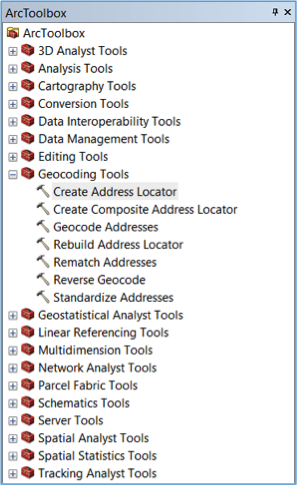
To create an address locator, use the “Create Address Locator” tool in ArcToolbox (see Figure 3.1).
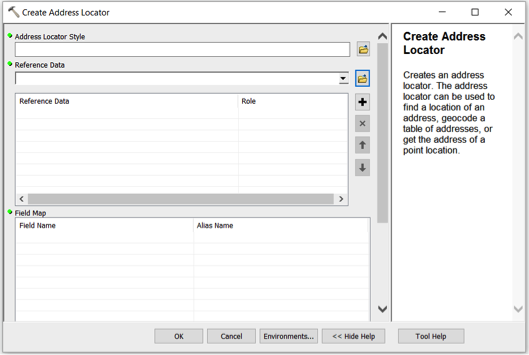
When you launch the tool, you are presented with the Address Locator dialog (see Figure 3.2).
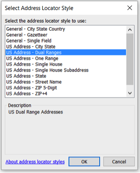
The first step in creating an address locator is selecting a locator style. The locator style which is most appropriate depends on the reference data you’re planning to use in addition to the format of the locations you’re trying to geocode. A commonly used address locator style is the U.S. Addresses – Dual Ranges (see Figure 3.3).
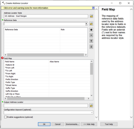
Once the locator style has been selected, the Field Map list in the bottom portion of the Address Locator dialog is automatically populated (see Figure 3.4). Fields with an asterisk are required by the locator style, and fields without an asterisk are optional. Once you have loaded a reference dataset, you can map these fields to the corresponding fields in the reference data.
The second step in creating an address locator is defining the reference dataset or datasets which will be used. As mentioned above, there are many reference data sources which can be used. For example, you can use a linear feature class based on roadway centerlines such as the “Address Range-Feature Shapefile” TIGER/Line shapefiles we reviewed in Lesson 2. Alternatively, you could use a polygon feature class based on parcel boundaries or zip code boundaries. Yet another option would be to use a point feature class based on address points.
Once you have selected the reference data, you can map the fields associated with the address locator style you have selected with the corresponding fields in the reference data (see Figure 3.5).
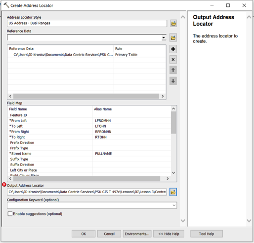
The final step is to save the address locator to a location you select. While you can store the locator in either a geodatabase or a file folder, ESRI recommends storing an address locator in a file folder for better performance.
Here is a link to an ESRI webpage where you can download a white paper [1] which tells you everything you’d ever want to know about address locators in ArcGIS.
Geocoding a List of Addresses (or other location descriptions)
To geocode a list of addresses, you should first add the table of addresses data to your map document in ArcGIS. The addresses to be geocoded can be prepared in any number of file formats including xlsx, xls, dbf, csv, and txt. Once the table of addresses has been added, you can right-click on the newly added table and select “Geocode Addresses” from the resulting context menu. At this point, you’ll be asked to select an address locator (see Figure 3.6).
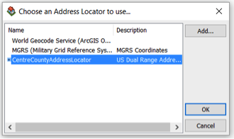
If the address locator you wish to use is not in the list, you can add it. Once you select an address locator and click “ok,” you will be presented with the “Geocode Addresses” dialog (see Figure 3.7).
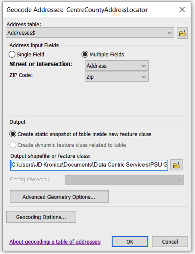
In the top portion of the dialog, you can map the fields in the input table to the corresponding fields in the address locator, if it isn’t done automatically, and define the location and name of the shapefile or feature class where the results of the geocoding process should be stored. You can also configure some parameters for the address locator by clicking the “Geocoding Options” button. The “Geocoding Options” dialog is then displayed (see Figure 3.8).
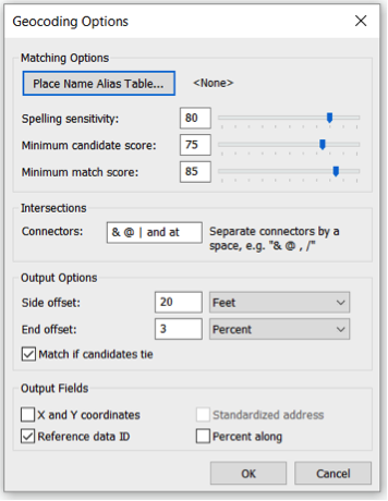
In the top portion of the dialog, you can exercise some control over how matching is performed. The spelling sensitivity level controls the extent to which misspellings will still be considered a match. The lower the score, the more tolerant the geocoding engine is for misspelled words. The minimum candidate score sets the threshold score for identifying candidates. The lower this score, the more candidates an address could have. Finally, the minimum match score establishes the threshold score for declaring a match for the address. Lowering the minimum match score will generally increase the match rate but will also tend to result in a higher rate of false positives.
The dialog can also be used to set other parameters for the geocoding engine such as offset positions for geocoded point features and some output data elements which can optionally be included as attributes in the resultant shapefile or feature class.
Once the geocoding options have been defined, the geocoding process can be initiated by clicking “Ok” on the “Geocode Addresses” dialog (see Figure 3.7). When the geocoding process is complete, a summary of the geocoding results is presented (see Figure 3.9).
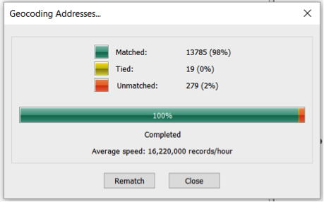
This summary shows the number of addresses which had candidates above the minimum match score (i.e., matches), the number of addresses which had multiple candidates which were above the minimum match score and had the same score (i.e., ties) and the number of addresses which did not produce any candidates above the minimum candidate score (i.e., unmatched).
From the results summary screen, a manual rematch process can be initiated by clicking the “Rematch” button. This brings up the “Interactive Rematch” screen (see Figure 3.10).
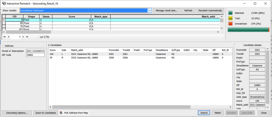
On this screen, unmatched addresses, ties, and matched addresses can be reviewed. Unmatched addresses generally result from either a problem with the address or a problem in the reference data. If a problem is observed with the address, it can be corrected and matched with the correct candidate directly on this screen. Often, however, it is unclear what the problem is with a particular address, and additional research is required to determine where the problem lies before it can be corrected.
3.2 Conflation
Conflation, in the context of GIS, is the process of combining two geospatial datasets so that the resultant dataset is superior to the input datasets. While conflation processes are used throughout GIS, they are of particular importance in GIS-T where roadway datasets of varying spatial quality and attribution are available from many different sources. The act of conflating datasets can often be a complex and time-consuming process. How complex and time-consuming the process is depends on a number of factors including the spatial extent of the datasets, the number of features present and the degree of spatial alignment between corresponding features. In some cases, it may be possible to automate a portion of the process but the success of these types of approaches depends on the quality of the initial datasets and the requirements for the final product.
Reference Dataset
When conflating two datasets, one of the datasets is generally considered to be the reference or target dataset. This is the dataset with the most spatially accurate features. The other dataset is sometimes referred to as the input or source dataset.
Conflation Workflow
While each conflation project can be unique, they all draw from a core set of activities. Some of the more common conflation activities include the following:
- Feature Matching: The objective here is to match corresponding features in the datasets. This process can be based on the spatial alignment of the features and/or certain attributes of the features.
- Feature Alignment: Once features are matched, they can be brought into spatial alignment with each other to establish proper topological relationships.
- Feature Addition: Features in the input dataset which are missing in the reference dataset can be added to the reference dataset.
- Attribute Transfer: Attributes information from the input dataset is added to the reference dataset.
The characteristics of the activities involved in a conflation project are largely dependent on the nature of the input datasets. There are three potentials scenarios:
- Vector - Vector
- Vector - Image/Raster
- Image/Raster - Image/Raster
In GIS-T, we are most commonly engaged in conflating two vector datasets (i.e., roadway data).
Horizontal Conflation vs. Vertical Conflation
Conflation can also be broadly categorized as horizontal conflation or vertical conflation based on the geographic relationship between the datasets. In horizontal conflation, the objective is to join two datasets which are spatially adjacent to each other. For example, perhaps you want to join roadway datasets from two adjacent counties or two adjacent states. In these cases, there is often some feature overlap near the dataset boundaries. In vertical conflation, the datasets being merged span the same geographic region or at least have substantial overlap. The objective is often to transfer a robust set of attribute data from one dataset, which may be of poor spatial accuracy, to a dataset which is poor in attribution but spatially accurate. Of course, in the real world, you may run across situations where the datasets partially overlap.
Conflation Tools
GIS software often has some built-in tools to at least assist with conflation needs. For example, in ArcMap 10.2.1, ESRI introduced a set of tools to help with conflation. The conflation toolset is found in the Editing Toolbox. ESRI also added a tool called Detect Feature Changes to the Data Comparison toolset in the Data Management Toolbox. Spend some time reviewing the help documentation for these tools.
3.3 Getting to Know a Transportation Organization
This week, we’ll take some time to explore Metropolitan Planning Organizations (MPOs) and Rural Planning Organizations (RPOs). MPOs were formed as part of 1962 Federal-Aid Highway Act and are required for any urbanized area with a population of more than 50,000. Congress recognized transportation planning is best done at a regional level since the nature of transportation systems and services often transcends an individual municipality, city, or county.
Watch the short video (11 minutes) below which discusses the purpose and structure of MPOs. There are more than 300 MPOs across the U.S., a listing of which is provided here [2].
Video: MPO Planning Process (11:27)
NARRATOR: Transportation is the backbone of our communities. We rely on it every day to get us to work, to get us to shopping and recreation, and to bring us goods and services. But who makes the decisions about our transportation system, and how are those decisions made? This video is an introduction to Metropolitan Transportation Planning and the role of metropolitan planning organizations.
Over the last 100 years or more, America's population and lines of commerce have expanded well beyond the boundaries of individual cities and towns. Today, networks of highways, transit services, freight carriers, and airports serve metropolitan areas that may include many cities, suburbs, towns, and counties. In today's urban areas, many transportation decisions are best handled at the regional level. A regional approach gives decision-makers a comprehensive understanding of transportation problems and the ability to develop comprehensive solutions.
Over the years, Congress has promoted a regional approach to urban transportation planning and decision-making. One of the most important advances came in the 1970s with legislation that required the creation of metropolitan planning organizations or MPOs in areas with a population of 50,000 or more. Now, there are over 300 MPOs across the country. An MPO may be a free-standing planning organization or an association of local governments, but every MPO is governed by a policy board of local elected officials. The Board may also include representatives from state transportation departments, mass transit operators, and others. The MPO is not alone in the decision-making process, but it's the engine that drives collaboration and cooperation among many participants. Local elected officials bring a unique perspective to the planning and decision-making process. They often face a challenging balancing act, making decisions that have the greatest regional benefit, while at the same time reflecting the concerns of the communities they represent.
MPOs and their partners produce three key documents: the Unified Planning Work Program, the Transportation Plan, and the Transportation Improvement Program. The Unified Planning Work Program (or UPWP) describes the planning studies that are being performed for the metropolitan area. The Transportation Plan identifies the region's transportation policies, strategies, and projects for the next twenty years or more. The Transportation Improvement Program (or TIP) is a short-range program of projects covering at least three years that directs available funds to those improvements that are the highest priority. The MPO Policy Board and its partners direct the development and content of the Plan, the TIP, and the UPWP. Both the Plan and the TIP must be fiscally constrained, in other words, consistent with available and expected funds. In areas with air quality problems, the Plan and the TIP must also help the region meet federal standards.
Let's now look at how the Plan and the TIP are prepared. Often the local planning participants start with a regional vision or a set of goals. This vision expresses what the region would like to become perhaps forty or fifty years in the future.
LES STERMAN: Well, important elements of a long-range plan are obviously a strong statement of goals and values, what is it that we're after, and transportation systems in the future.
NARRATOR: In developing a vision or goals, the MPO may consider many questions: What are the trends in regional growth, and are they desirable? How well is the transportation system performing? Do existing plans deal with current and expected problems? Can the transportation system support the kinds of future development that the region desires? When the vision and goals are in place, the MPO and its partners are better able to identify transportation problems and needs. These can include declining mobility, increasing congestion, poor access to jobs in neighborhoods, unhealthy air, or inconsistency with proposed economic development. An understanding of these problems allows the MPO and its partners to identify alternatives to improve transportation. Alternatives may include new policies, operational strategies, or capital projects. Some may help the existing system work better. Others may expand or build new transit lines, highways, and other facilities. Another round of questions is asked in assessing the impact of alternatives. How well does each alternative address the region's transportation problems? What are the likely impacts on neighborhoods and the environment? How much do the alternatives cost? Are the funds there, and is this the best use of available resources? The answers to these questions help the board choose the best alternatives. By adopting the Transportation Plan, the board establishes the policies, strategies, and projects that the region will pursue.
To develop the TIP, priority projects are drawn from the adopted Transportation Plan and matched with available funding. Once adopted by the MPO, the TIP is submitted to the state and becomes part of the statewide transportation improvement program, but the process doesn't end here. Projects and strategies in the plan and TIP undergo further development, often including engineering and environmental studies. Also, many MPOs monitor the implementation of the plan and TIP, study how well the plan is working, and make periodic adjustments. Federal rules require that the plan be updated and readopted every three to five years, and the TIP every two years.
RAE RUPP SRCH: Long-range planning, it is an ongoing process. It's not etched in stone, and many people don't realize that. New board members don't realize that either, that it's not a plan etched in stone. That, you know, it's constantly in an updating process.
NARRATOR: Agency and public involvement is a key activity in every step of the planning process. The public refers to a variety of individuals, agencies, and organizations each with different interests and levels of involvement. Many different approaches are used to inform and engage other agencies and the public.
CHARLES UKEGBU: Our public participation is not just at the MPO level, and that's one of the things we try to emphasize at the municipal level. It is not just the MPO calling a meeting, no, it is the MPO participating in other meetings and forums that may have been called by other, whether city or state agencies.
NARRATOR: Transportation planning continues to evolve. New issues are emerging that demand innovation and creativity from MPOs. Many MPOs today are working with other local and state agencies and the private sector to provide multi-modal systems that give people more choices. Transit, carpooling, bicycling, walking, better connections between highways, transit, airports, freight, and other modes of transportation can make the entire system work more efficiently.
DAVID PAMPU: We can't solve our transportation problem in key corridors just by widening the roads anymore. We have to provide some additional mobile opportunities for the traveling public. By focusing on rapid transit in conjunction with roadway improvements, we think we can add significant capacity for the traveling public.
NARRATOR: Coordinating transportation and land-use can be challenging. While transportation decisions are made at the state and regional levels, most land use decisions are made by local governments and private developers. The MPO may be the only place where officials from different jurisdictions can coordinate land use and transportation planning for the region as a whole. Many MPOs are partnering with state transportation departments, transit operators, and other agencies to preserve existing transportation assets and to squeeze more capacity out of their existing systems.
LES STERMAN: Probably for forty years, we chased congestion. Congestion was our number one goal, addressing congestion was our number one goal. But now we're recognizing that preserving existing system, our bridges and highways and our transit systems and the safety of that system are in fact more important goals, and we recognize them, and that's part of our vision. To create a system that's not only safe but is well maintained and preserved particularly in the core of our region.
NARRATOR: Planners are also making greater efforts to respond to the needs of all the users of transportation systems. People of every age, ethnic group, and income level because mobility is a link to opportunity and equality. For elected officials and citizens alike, Metropolitan Transportation Planning is a tremendous opportunity to build better communities.
JEFFREY SCHIELKE: I think I went into it not realizing, you know, that I was in a much wider, bigger area that had dramatic impacts until I got in the process and began to experience, you know, what other towns were going through and seeing and learning from their mistakes and learning their ideas. I think that's one of the rich rewards of the MPO process.
RAE RUPP SRCH: It's an exciting position to be in. You do have input, you're representing your communities. I think anybody that wants to get involved in this should.
JOHN MASON: It is basically a collaborative approach among the jurisdictions within a metropolitan region. There are some federal rules and laws that guide how we have to go through the process, but the real success of MPOs is based on the ability of the leaders of the jurisdictions to be able to collaborate to achieve a common goal.
Rural areas often have transportation needs that are very different from metropolitan areas. In rural regions, either the State DOT, a Rural Planning Organization (RPO), or a local government conducts transportation planning. While RPOs are not federally required, it is a requirement that if the state performs the planning function for rural regions, they need to coordinate with local officials.
In Pennsylvania, there are 15 MPOs and 8 RPOs. MPOs and RPOs often have strong GIS capabilities to support various planning studies.
3.4 Getting to Know Each Other
This week you’ll have a one-on-one chat with one of your classmates as per the schedule you were provided in Week 1. The discussion should be at least 30 minutes in length. If it’s the first time you’ve chatted with each other, spend the majority of time getting to know each other. Otherwise, focus on discussing the lesson content.
3.5 Webinar for Next Week
Speaker
Next week, our speaker will be Mr. Glenn McNichol. Glenn is a Senior GIS Specialist with the Delaware Valley Regional Planning Commission (DVRPC). He has been with the Commission for 23 years. As a member of DVRPC’s GIS unit, he supports the activities of the Commission’s planning staff through map production, data development, and GIS analysis. He also manages the Commission’s orthoimagery program.
Glenn holds a BA in Geography from Montclair State University. He also received a Professional Certificate in Geomatics from Cook College, Rutgers University.
The August 2016 edition of DVRPC News [4] featured a profile of Glenn (note: scroll to the bottom of the page to see the profile).
The Delaware Valley Regional Planning Commission (DVRPC)
DVRPC is a Municipal Planning Organization (MPO) responsible for 9 counties in the Philadelphia area, 6 of which are in Pennsylvania and 3 of which are in New Jersey.
DVRPC's stated vision and mission statements are shown below:
DVRPC’s vision for the Greater Philadelphia Region is a prosperous, innovative, equitable, resilient, and sustainable region that increases mobility choices by investing in a safe and modern transportation system; that protects and preserves our natural resources while creating healthy communities, and that fosters greater opportunities for all.
DVRPC’s mission is to achieve this vision by convening the widest array of partners to inform and facilitate data-driven decision-making. We are engaged across the region, and strive to be leaders and innovators, exploring new ideas and creating best practices.
DVRPC is engaged in many transportation projects [5]. Spend some time looking through a few of them.
3.6 Summary of Lesson 3
In this lesson, we discussed a number of geocoding techniques and considered the pros and cons of each. We also examined the properties of an address locator in ArcGIS and the role it plays in the geocoding process. You had the opportunity to construct your own address locator using TIGER/Line shapefiles and used it to geocode a series of addresses.
We also learned a bit about conflation especially in regards to roadway datasets. You then explored some of the tools in ArcGIS which can be used to conflate multiple datasets.
Our transportation organizations of the week were MPOs and RPOs. We learned about how they are structured and the responsibilities they have in the area of transportation planning.
In our weekly webinar, we had the opportunity to interact with Dr. Ira Beckerman, an archaeologist who leads PennDOT’s cultural resources group which is responsible for the Department’s compliance with Section 106 of the National Historic Preservation Act. We also had the opportunity to hear from Glenn McNichol, a Senior GIS Specialist with the Delaware Valley Regional Planning Commission (DVRPC).
In preparation for next week’s webinar, we took a look at DVRPC, a large MPO which handles the Philadelphia area, and explored the types of transportation projects they conduct.
Finally, you had the opportunity to get to know one of your classmates a little better and share some of your ideas and questions about this week’s lesson materials.
Questions and Comments
If there is anything in the Lesson 3 materials about which you would like to ask a question or provide a comment, submit a posting to the Lesson 3 Questions and Comments discussion. Also, review others’ postings to this discussion and respond if you have something to offer or if you are able to help.