Lesson 4: Transportation Networks
Learning Outcomes
What will we learn?
By the end of Lesson 4, you should be able to:
- describe the importance of a transportation network;
- characterize the data elements which go into a street network and evaluate street data sources to determine their suitability in serving as the basis of a network dataset;
- create a network dataset from street data;
- list the key functions of the Federal Highways Administration (FHWA);
- describe the composition and purpose of the National Highway System (NHS);
- discuss FHWA’s Geospatial Data Collaboration (GDC) initiative; and
- talk about the importance of addressing environmental and community considerations early in the transportation planning process and provide some examples of how GIS can be used to facilitate this process.
4.1 Transportation Networks
People and goods can move from one location to another by traversing a transportation network. There are many types of transportation networks including street networks, railroad networks, pedestrian walkway networks, river networks, utility networks, and pipeline networks. A geospatial model of a transportation network is comprised of linear features and the points of intersection between them. The modeling and analysis of networks has so many applications that there is an entire branch of mathematics devoted to it known as graph theory. In graph theory, linear segments of the network (e.g., road segments) are referred to as edges, and the points where the linear segments connect are called nodes.
Some transportation networks permit travel in both directions such as street networks and are referred to as undirected networks. Other networks generally limit travel to a single direction such as pipeline networks. These networks are referred to as directed networks. In ArcGIS, undirected networks are modeled with network datasets whereas directed networks are modeled as geometric networks. In this course, we will limit our study to street networks and the use of network datasets to model them.
Many transportation problems can be addressed through a network. A few examples are listed below:
- identifying the fastest, shortest, or most scenic path between two points on the network;
- determining the most efficient way for a delivery vehicle to visit a series of stops (also known as the traveling salesman problem);
- defining the service area around a given location;
- identifying an optimal store location.
We will take a detailed look at some of the more common network analyses in the next lesson. In this lesson, we will focus on the components of a transportation network model and the mechanics of creating one.
While a high-quality set of roadway centerline data is certainly a prerequisite to modeling a transportation network, it is by no means sufficient. Other important elements of a network model include the following:
-
Topology
The topology of a street network refers to the spatial arrangement and connectivity of the roads which comprise the network. Understanding how the road features relate and connect is critical to determining which paths or routes through the network are possible. Elevation is an important consideration in establishing network topology. Physical connections between streets require not only that they cross in the x-y plane but also that they cross at the same elevation. The picture below shows a complex interchange where many roads cross, but there are limited points of connectivity.
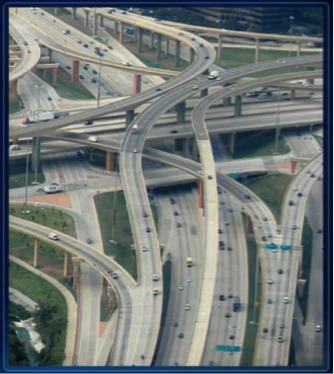 Figure 4.1: Complex Highway InterchangeCredit: ESRI 2010 User Conference Technical Workshop
 -
Cost Attributes
In order to select the “best” route between two points in a network, you need to define what you are trying to accomplish. Perhaps you’re interested in determining the shortest route. In this case, you would need to know the distance between all adjacent nodes in the network. Consequently, the edges would need to have an attribute which quantifies length. Alternatively, if you want to know the fastest route between two points, you need to know the time it takes to move between any two adjacent nodes. Consequently, to support the fastest route determination, the edges need to have an associated time attribute or a speed limit attribute, since time is a function of length and speed limit. Regardless of how you define “best,” you need to have a corresponding attribute or attributes which allow the cost of potential routes to be quantified and compared. For example, if you want to know the most scenic route between any two points in the network, you would need to have a scenic score attribute associated with each edge which quantifies its scenic value.
-
Turns
Turns also play a key role in modeling a street network. One fundamental consideration in regards to turns is whether they are permitted. Many road intersections do not permit U-turns, for example. A second consideration for turns is the length of time they take. Left turns generally take longer to complete than right turns, since you generally have to contend with oncoming traffic. In order to accurately estimate how long it would take to traverse a network along a specific route, turn delays need to be taken into account.
-
One-Way Restrictions
Another important data element for a street network relates to one-way roads. In order to ensure that only legitimate routes are considered, roads which limit travel to one direction need to be identified.
-
Traffic
We all know that traffic plays an important role in determining how long it takes to traverse a particular route. Consequently, historic traffic data, or better yet, live traffic data, can be extremely useful in a street network model.
-
Directions
Often one of the desired outputs of network analysis is a set of description directions. In order to support the production of meaningful directions, a variety of descriptive roadway attributes needs to be present. Signpost data can also provide a valuable source of information for the creation of meaningful directions.
As you can see, a lot of information is required beyond basic roadway centerline geometry in order to create a street network which can support network analysis and produce high-quality results.
4.2 Getting to Know a Transportation Organization
This week, you’ll take some time to get to know the Federal Highways Administration (FHWA), an important agency within the USDOT. The roots of the FHWA trace back to its first predecessor organization known as the Office of Road Inquiry (ORI) which was created by President Grover Cleveland in 1893. In the days before the automobile, interstate travel was dominated by railroad and it was actually a bicycle boom which was largely behind the initial interest in improving America’s roads. An interesting history of the FHWA can be found here [1]. A signature achievement in the advancement of America’s roads was the development of the Interstate system of roadways championed by President Dwight D. Eisenhower. Today, the Interstate system represents about 50,000 miles of highway and is responsible for about one-quarter of the vehicle miles traveled on America’s roadways.
The primary function of the FHWA is to assist states and local governments with the design, construction, and maintenance of roads and bridges and to ensure US roads and highways meet a high standard of safety and quality. The primary mechanism through which the FHWA supports states and local governments is the Federal Aid Program. This program looks to focus federal monies on the nation’s most important roadways.
The Intermodal Surface Transportation Efficiency Act of 1991 introduced the concept of the National Highway System, a system of roads and highways deemed critical to America’s economy, defense, and/or mobility. Through the efforts of FHWA working with other federal, state, and local partners, roughly 160,000 miles of roadway were identified for inclusion in the NHS. The National Highway System Designation Act of 1995 signed into law by President Bill Clinton officially designated these roadways as the NHS.
A brief but informative article on the NHS titled The National Highway System: A Commitment to America's Future [2] appeared in a 1996 edition of Public Roads, a bimonthly magazine published by FHWA.
One of the FHWA’s key objectives is to encourage innovation and to provide states and local governments with needed technical assistance. A recent FHWA initiative known as Geospatial Data Collaboration [3] (GDC) is aimed at promoting the use of GIS tools to facilitate data sharing and increased collaboration between transportation agencies and resource agencies, with the ultimate objective of more timely project delivery.
4.3 Getting to Know Each Other
There are no one-on-ones scheduled for this week.
4.4 Webinar for Next Week
Next week we'll hear from 2 speakers.
Speaker #1
Our first speaker will be Mr. Frank DeSendi. Frank is the Manager of PennDOT’s Geographic Information Division and is also a former Chair of the American Association of State Highway Transportation Officials’ GIS for Transportation (AASHTO GIS-T) Task Force. He began his career with PennDOT in 1989 and has been working in the geospatial field since 1995. Frank holds a Bachelor of Science in Geography from The Pennsylvania State University.
One interesting use of spatial technology which Frank’s group implemented a few years ago is called LPN which stands for Linking Planning and NEPA. PennDOT and its planning partners (i.e., the MPOs and RPOs) use the application to screen potential projects against more than forty environmental datasets which collectively address most NEPA concerns. Based on the proximity of a proposed transportation project to these resources, the application determines a score which can be used to compare various alternatives for the project. The user’s guide for the application is here [4].
Planning and Environmental Linkages (PEL)
In the past, transportation planning and the development of TIPs and STIPs occurred with little thought given to environmental and cultural resources and community concerns. Later in the project development process, when the design and construction of the project were imminent, the potential impacts to these resources were considered as is required by NEPA. If through this NEPA review process, the project was anticipated to have potential impacts on these resources, it often led to substantial delays in project delivery, unexpected increases in the project budget, and a less than ideal solution for all involved. Consequently, significant efforts have been made in the past 15 years to begin assessing potential impacts to resources early in the planning process and for transportation agencies to work more closely with resources agencies. Spatial technologies have played a large role in facilitating potential impact assessments, identifying alternatives that eliminate or minimize impacts and, when impacts are unavoidable, identifying mitigation strategies which can offset any negative impacts of the project.
In response to the need to more closely integrate transportation planning and environmental review, FHWA created the Planning and Environmental Linkages (PEL) program to help state DOTs, MPOs and RPOs revise their planning processes, improve their coordination with resource agencies and develop tools to streamline the entire process.
Watch the 2011 webinar (72 minutes) jointly sponsored by FHWA and AASHTO titled Linking Transportation and Natural Resource Planning through the use of Environmental GIS Tools [5].
Speaker #2
Our second speaker will be Mr. Greg Ulp. Greg is a Senior Project Manager with GeoDecisions, a division of Gannett Fleming specializing in GIS and IT. He has over 25 years of experience in applying spatial technologies to solve transportation problems and has worked with a number of state DOTs. Greg has worked extensively with the Pennsylvania Department of Transportation’s GIS Division. He was the technical architect for a GIS application called the Multimodal Project Management System Interactive Query (MPMS-IQ) which is used to access and visualize data for the Department’s highway and bridge projects. Greg holds a bachelor’s degree in computer science from The Pennsylvania State University.
Transportation Planning
There are a number of transportation plans that regional planning organizations (MPOs and RPOs) and state DOTs are federally required to prepare and periodically update. These include the following:
- Long Range Transportation Plan (LRTP)
An LRTP, also known as a Regional Transportation Plan (RTP), is a long-term plan which is prepared by an MPO. It typically has a 20 to 30-year horizon and is updated every 3 to 5 years. The LRTP establishes priorities and long-term objectives for the region. - Transportation Improvement Program (TIP)
The TIP is a short-term plan, at least 4 years in length, which aligns with the policies and objectives defined in the LRTP. Each MPO is federally mandated (49 U.S.C. 5303(j)) to develop a TIP which includes all federally funded projects in addition to non-federally funded projects which are consistent with the LRTP. The TIP is required to be in line with available funding (i.e., fiscally constrained). - Statewide Transportation Improvement Program (STIP)
The STIP is a statewide roll-up of each of the TIPs across the state and is maintained and updated by the state DOT. The STIP is also federally mandated (23 U.S. Code § 135). Each state’s STIP is subject to approval by both the Federal Highways Administration (FHWA) and the Federal Transit Administration (FTA) (two organizations we’ll take a look at in upcoming lessons).
Project Visualization Tools
In order to solicit feedback from the public on potential projects and to provide legislators and the public access to information on planned and active projects, state DOTs, Municipal Planning Organizations (MPOs) and Rural Planning Organizations (RPOs) sometimes use web-based GIS applications to enable people to visualize projects in a specific geographic area and get detailed information on a project of interest.
Watch this FHWA sponsored webcast on Visualizing TIPs and STIPs Using GIS [6] which was held on April 27, 2016. It is a little rough in spots but is very informative. The presentation doesn’t actually start until about 7 ½ minutes in, due to some technical difficulties. In the webcast, PennDOT discusses three separate GIS-based project visualization applications which are used to provide the public and state legislators access to planned and active projects. All three applications have a consistent user interface and differ only in the types of projects they show. The first application shows active projects under construction, the second shows Act 89 projects which are projects of particular interest to state legislators and the third shows planned projects (i.e., projects on the STIP and TYP). All three applications can be accessed here [7].
Another organization which participated in the webcast was the Delaware Valley Planning Commission (DVRPC). DVRPC is an MPO which spans 9 counties in 3 states (Pennsylvania, New Jersey, and Delaware). In the webcast, DVRPC discusses how they make project information available through a Google Maps-based GIS application. Take some time to explore the 2017 DVPC TIP Visualization tool [8]. In addition to using GIS to facilitate visualization of their transportation program, DVRPC also uses spatial technologies to evaluate potential projects for the TIP based on a variety of criteria they have developed.
MPMS-IQ
MPMS-IQ is a web-based GIS application developed for PennDOT which allows users to visualize projects and access a wide variety of project related information via a map interface. The projects which are available through MPMS-IQ include active construction projects in addition to projects on PennDOT’s Twelve Year Plan (TYP). Unlike the STIP, the TYP is not federally mandated. The STIP corresponds to the first 4 years of the TYP. Take some time to explore MPMS-IQ [9]. In particular, look at the methods by which users can search for projects, the information available for each project, and the additional layers and features the application provides.
Additional Learning
TELUS is a research and innovation program funded through a grant from the FHWA designed to create spatially-enabled tools to assist MPOs and state DOTs in preparing TIPs and performing other transportation planning functions. TELUS software is created and maintained by the New Jersey Institute of Technology (NJIT). Information about the tools, including demos and download links, can be found here. [10]
4.5 Summary of Lesson 4
In this lesson, we learned about transportation networks. Specifically, we examined the elements which comprise a network and the activities that go into creating one. You then had the opportunity to solidify this knowledge by modeling a transportation network in ArcGIS through the construction of a network dataset from roadway centerlines and other associated data.
Our transportation organization of the week was the FHWA. You learned a little about the history and key roles of the FHWA. We also took a look at NHS, a network of roadways deemed critical to the nation, and FHWA’s geospatial data initiative known as the GDC.
We also had the opportunity to hear from two speakers this week. Glenn McNichol, a Senior GIS Specialist with the Delaware Valley Regional Planning Commission (DVRPC) and Michael Ratcliffe, the Assistant Division Chief for Geographic Standards, Criteria, Research, and Quality in the Census Bureau’s Geography Division.
In preparation for next week’s webinars, we learned how transportation planning and the NEPA review processes which seek to assess and mitigate environmental impacts related to transportation projects have become more tightly integrated and about the role GIS has played in helping to bring the two together. We also took a look at some GIS applications used to visualize planned and active transportation projects.
Questions and Comments
If there is anything in the Lesson 4 materials about which you would like to ask a question or provide a comment, submit a posting to the Lesson 4 Questions and Comments discussion. Also, review others’ postings to this discussion and respond if you have something to offer or if you are able to help.