Lesson 1: The GPS Signal
The links below provide an outline of the material for this lesson. Be sure to carefully read through the entire lesson before returning to Canvas to submit your assignments.
Lesson 1 Overview
Overview
About 35 years ago, I read in a trade publication about an event that might have seemed unremarkable to many at the time. A company in the Northeast had agreed to sell the Macrometer to a company in Houston. I was exhilarated. I immediately wrote to the company in Houston and said, “Now that you have the Macrometer, you will undoubtedly need people to operate it. Virtually no one knows anything about it, including me. So you will have to train whomever you hire. How about training me?”
I will always be grateful that they agreed to do so. So, in a matter of months, I found myself leading a crew that did work around the world with the very first operational GPS receiver, the Macrometer.
The Macrometer was a codeless receiver. There are no receivers today that use that particular approach. Most utilize both the code and carrier from the GPS signal. Do the receivers you have used track both? Many consumer grade GPS receivers are code-phase only. Is that an advantage or a disadvantage when it comes to accuracy? You will learn the answers to these questions and many more in the first lesson of this course.
Objectives
At the successful completion of this lesson, students should be able to:
- demonstrate understanding of the basic GPS signal structure;
- discuss the similarities between GPS and trilateration;
- describe the pertinence of the navigation code;
- explain the structure of the P and C/A codes;
- define the creation of the GPS modulated carrier wave;
- identify the two GPS Observables;
- describe the role of autocorrelation and the lock and time shift associated with GPS pseudoranging;
- recognize the pseudorange equation (This is code phase);
- discuss the role of carrier phase ranging in high accuracy GPS.
Questions?
If you have any questions now or at any point during this week, please feel free to post them to the Lesson 1 Discussions Forum. (To access the forum, return to Canvas and navigate to the Lesson 1 Discussion Forum in the Lesson 1 module.) While you are there, feel free to post your own responses if you, too, are able to help out a classmate.
Checklist
Lesson 1 is one week in length. (See the Calendar in Canvas for specific due dates.) To finish this lesson, you must complete the activities listed below. You may find it useful to print this page out first so that you can follow along with the directions.
| Step | Activity | Access/Directions |
|---|---|---|
| 1 | Read the lesson Overview and Checklist. | You are in the Lesson 1 online content now. The Overview page is previous to this page, and you are on the Checklist page right now. |
| 2 | Read the lecture material for this lesson. | You are currently on the Checklist page. Click on the links at the bottom of the page to continue to the next page, to return to the previous page, or to go to the top of the lesson. You can also navigate the lecture material via the links in the Lessons menu. |
| 3 | Read Chapter 1 in GPS for Land Surveyors. | GPS for Land Surveyors is the required textbook. |
| 4 | Participate in the Discussion. | To participate in the discussion, please go to the Lesson 1 Discussion Forum in Canvas. (That forum can be accessed at any time by going to the GEOG 862 course in Canvas and then looking inside the Lesson 1 module.) |
| 5 | Read lesson Summary. | The lesson Summary is the last page in this lesson. |
Introduction
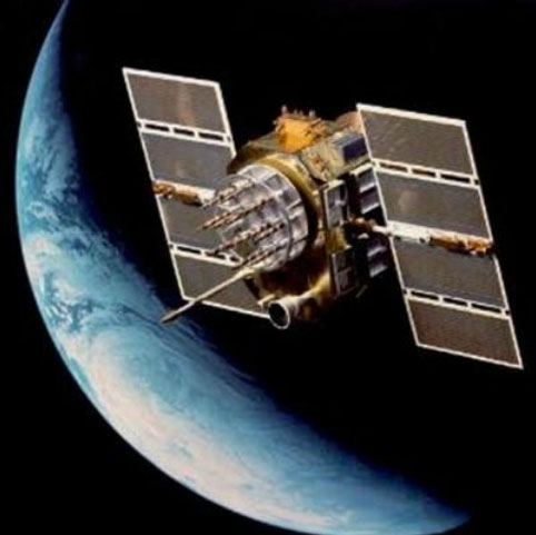
Hello, my name is Jan Van Sickle and I would like to welcome you to the GPS course. The first image here is a representation of the Block IIR/IIR-M/IIF satellites that make up the majority of the current constellation of GPS satellites. In this first lesson, we will be talking about the GPS signal. I think it is a good place to begin, because it gives you a general idea of how GPS functions, how positions are derived from the system. This capability, of course, is at the heart of the application of GPS to various components.
Trilateration
GPS can be compared to trilateration. Both techniques rely exclusively on the measurement of distances to fix positions. One of the differences between them, however, is that the distances, called ranges in GPS, are not measured to control points on the surface of the earth. Instead, they are measured to satellites orbiting in nearly circular orbits at a nominal altitude of about 20,183 km above the earth.
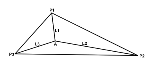
GPS is often compared to triangulation, which is actually not entirely correct. More correct would be trilateration. Trilateration is based upon distances rather than the intersection of lines based on angles. Now, in a terrestrial survey as indicated in this image here, there would probably be a minimum of three control stations, and from them would emanate three intersecting distances, i.e., L1, L2, and L3.
This is very similar to what's done with GPS, except instead of the control points being on the surface of the Earth, they are orbiting the Earth. The GPS satellites are the control points orbiting about 20,000 kilometers above the Earth. There's another difference; instead of there being three lines intersecting at the unknown point, there are four. Four are needed because there are four unknowns - X, Y, Z, and time - that need to be resolved.
There are also some similarities between this image of terrestrial surveying and the GPS solution. The distances need to be paired with their correct control points in both cases. Another is that the distances are measured electronically based upon the speed of electromagnetic radiation (i.e. light) and the amount of time that the signal takes to go from the control point to the unknown point, and back in some cases. Please note that in GPS that trip is one way. We'll talk more about that. There are other similarities too, but these ideas of distances being used, several simultaneous distances, being used to find the position of an unknown point is one of the fundamental ideas behind the functioning of GPS.
Unknowns
Time
Time measurement is essential to GPS surveying in several ways. For example, the determination of ranges, like distance measurement in a modern trilateration survey, is done electronically. In both cases, distance is a function of the speed of an electromagnetic signal of stable frequency and elapsed time.
Control
Both GPS surveys and trilateration surveys begin from control points. In GPS, the control points are the satellites themselves; therefore, knowledge of the satellite's position is critical.
A Passive System
The ranges are measured with signals that are broadcast from the GPS satellites to the GPS receivers in the microwave part of the electromagnetic spectrum; this is sometimes called a passive system. GPS is passive in the general sense that the satellites transmit signals; the users receive them. That situation at a GPS receiver is similar to a car radio receiver. It doesn't send and, in that sense, is passive.
I mentioned that time is one of the unknowns that needs to be resolved to provide a position on the Earth using GPS. The measurement of time is essential. For example, the time elapsed for the electromagnetic signal to travel from the satellite to the receiver is important. Moments of time are also important. There are several clocks (oscillators) associated with the systems, both in GPS satellites and in GPS receivers.
As mentioned earlier, both GPS and trilateration surveys, on the terrestrial side, have to have control points. In the image here, the satellites themselves are the control points, so it's important to know where the satellite is in the sky at the moment that a measurement is taken. This is the purpose of the ephemeris of the satellite.
One-way Ranging
A GPS signal must somehow communicate to its receiver:
- what time it is on the satellite,
- the instantaneous position of a moving satellite,
- some information about necessary atmospheric corrections, and
- some sort of satellite identification system to tell the receiver where it came from and where the receiver may find the other satellites.
If we are to measure distances from the satellite to the receiver, and that is the foundation of GPS survey, some information needs to be communicated from the satellite to the receiver and that information needs to come along with the signal from the satellite to the receiver.
One aspect is the time on the satellite, because, of course, the elapsed time that the signal spends going from one place to the other is the basis of the distance measurement - ranging. Therefore, it is important to know the time on the satellite the instant that the signal left.
Secondly, the position of the moving satellite at an instant is critical. The coordinate of the satellite at that moment of measurement is important so that it can be used to derive the position of the receiver. In a terrestrial survey, instantaneous position hardly comes into it because the instrument on the control point is stationary on the Earth's surface. Satellites, on the other hand, are moving at a pretty tremendous rate of speed relative to the GPS receiver, so the ephemeris needs to provide the coordinates of the satellites at an instant of time. This is another way that time is important.
Some information about the atmosphere needs to be communicated to the receiver, too. If you're familiar with electronic distance measurement (EDM) surveying, you know that when an electromagnetic signal goes through the atmosphere, it is attenuated by the humidity, the temperature, and the barometric pressure. Therefore, these data are introduced into the processing of the distances that are measured with EDM instruments.
The GPS signal is going through a good deal more of the atmosphere than even the longest EDM shot. The first component of the atmosphere that the GPS signal encounters is the ionosphere. The ionosphere has some characteristics that differ from the next atmospheric layer the signal encounters, the troposphere. In any case, the signal can be attenuated rather dramatically during its trip. It follows that it is important to have some representation of the atmosphere through which the signal is passing communicated to the GPS receiver from the satellite. This is so that the resultant delays can be introduced into the calculation of the GPS derived position of the receiver.
Some sort of satellite identification system is required, too. Each distance that the receiver measures from each satellite must be correlated to that satellite. Since the receiver will need to have at least four distances from at least four different satellites, it needs to be able to assign the appropriate range, the appropriate distance or length, to the correct satellite. It needs to identify the origin of each signal.
This is just some of the information that needs to come down on that signal from the satellite to the receiver. It's quite a list, and is actually even a little bit longer than this.
The Navigation Message
| Subframe | 1 word | 2 words | 3-10 words |
|---|---|---|---|
| 1 | TLM | How | Clock correction, GPS week, Satellite Health, etc. |
| 2 | TLM | How | Ephemeris |
| 3 | TLM | How | Ephemeris |
| 4 | TLM | How | Ionosphere, PRN 25-32 Satellite Almanac and Health, UTC, etc. (Subframe 4 contains 25 subcommutated pages) |
| 5 | TLM | How | PRN 1-24 Satellite Almanac and Health, etc. (Subframe 5 contains 25 subcommutated pages) |
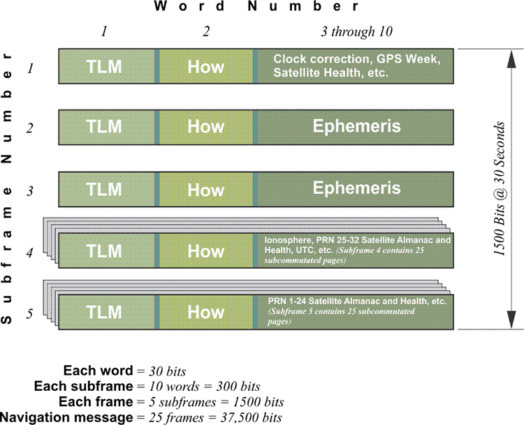
This is the primary vehicle for communicating the NAV message to GPS receivers. The NAV message is also known as the GPS message. It includes some of the information the receivers need to determine positions. Today, there are several NAV messages being broadcast by GPS satellites, but we will look at the oldest of them first. The legacy NAV (NAV) message continues to be one of the mainstays on which GPS relies. The NAV code is broadcast at a low frequency of 50 Hz on both the L1 and the L2 GPS carriers. It carries information about the location of the GPS satellites called the ephemeris and data used in both time conversions and offsets called clock corrections. Both GPS satellites and receivers have clocks on board. It also communicates the health of the satellites on orbit and information about the ionosphere. The ionosphere, along with the troposphere, is a layer of atmosphere through which the GPS signals must travel to get to the user. It includes data called almanacs that provide a GPS receiver with enough little snippets of ephemeris information to calculate the coordinates of all the satellites in the constellation with an approximate accuracy of a couple of kilometers. The Navigation code, or message, is the vehicle for telling the GPS receivers some of the most important things they need to know. Here are some of the parameters of its design.
The entire Navigation message, the Master Frame, contains 25 frames. Each frame is 1500 bits long and is divided into five subframes. Each subframe contains 10 words, and each word is comprised of 30 bits. Therefore, the entire Navigation message contains 37,500 bits and at a rate of 50 bits-per-second takes 12½ minutes to broadcast and to receive on a completely cold start. In other words, getting the whole thing is not instantaneous. It does take a bit of time for the receiver to update its Navigation Message.
In the five sub-frames of the legacy Navigation Message. TLM stands for telemetry. HOW stands for handover word. Over on the right-hand side in the illustration, you see the clock correction, GPS satellite health, et cetera, in sub frame one. Two and three are devoted to the ephemeris. In four and five, you see ionosphere, and then PRN (Pseudo Random Noise) satellite numbers and almanac are mentioned. The PRN term is used because the GPS signals that the receiver uses for positioning appear to be random noise, but in fact, the signal is pseudo (false) random noise because in truth, the signals are very carefully designed and consistent. They are not noise at all. They just seem to be irregular. The PRN numbers 25 to 32 in sub-frame number four mean that satellite's almanacs from number 25 to number 32 are to be found there. In subframe five the PRNs from 1 to 24, those satellites have their almanacs, in other words, a little bit of their ephemerides. You might wonder why they are there. This is that identification system. In other words, when a receiver acquires the Navigation Message from one satellite - embedded in that message - there's a bit of information, just a bit, that will tell the receiver where it can find the rest of the entire constellation in the sky. This helps it acquire the additional satellites after it's got the first one. That's what the satellite almanac does.
The essential point here is that this message is the fundamental vehicle for the satellite to communicate important information to the receiver. After the receiver has acquired the signal from that satellite, the NAV message tells the receiver where the satellite is. The ephemeris is the satellite coordinate system. It tells the receiver where the satellite is at an instant of time. The clock correction is one of the ways that the satellite can tell the receiver what time it is on-board the satellite. The ionosphere is that information that will allow the receiver to make some atmospheric corrections on the signal it receives from a particular satellite.
The Control Segment
Unfortunately, the accuracy of some aspects of the information included in the NAV message deteriorates with time. Translated into the rate of change in the three-dimensional position of a GPS receiver, it is about 4 cm per minute. Therefore, mechanisms are in place to prevent the message from getting too old. For example, every two hours, the data in subframes 1, 2 and 3, the ephemeris and clock's parameters, are updated. The data in subframes 4 and 5, the almanacs, are renewed every six days. These updates are provided by the government uploading facilities around the world which are known, along with their tracking and computing counterparts, as the Control Segment. The information sent to each satellite from the Control Segment makes its way through the satellites and back to the users in the NAV message.
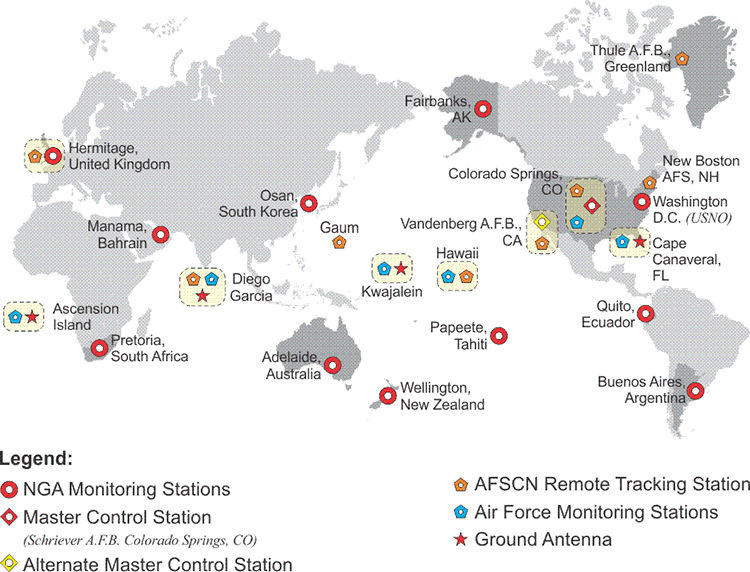
The question might arise in your mind, where does this Navigation Message and the information embedded there come from? It comes from the Control Segment. There are three segments in the GPS system: the User Segment, the Control Segment, and the Space Segment. The Space Segment is obviously the satellites themselves, the User Segment are all of us with our GPS receivers, and the Control Segment, well, here's an illustration that shows you the expanded Control Segment that is currently operational.
It's a good thing that we have the Control Segment a little bit modernized from what it once was. We'll talk more about that in the future, but here we have the stations, some of them monitor stations and then some of them actually have upload capability as well. In general, what happens is this. The GPS satellites are tracked by at least, now, three of these stations simultaneously all the time. Now, by tracking them, they are able to do several things. For example, since the stations already know their positions on the surface of the Earth, they are able to collect the signals from the satellites and know how much they have been delayed or attenuated by the atmosphere. They're also able to track the satellites and determine their path, their orbit. From this, their ephemerides can be calculated. The control station is also able to compare the signal coming from the satellite with the station's atomic clock, see the difference between the two, and then upload a clock correction to the satellite.
This is basically how the information is derived. It then goes from the tracking stations to the Master Control Station in Colorado Springs at Schriever Air Force Base, where calculations are done and the components that we've just seen in the Navigation Message are generated.
Those corrections go back to the upload stations with the ground antennas and are uploaded back to the satellites. That's where the information that is in the Navigation Message comes from. It's the control stations in the Control Segment on the surface of the Earth comparing the received signal from the satellite with their satellite clock, with their atomic clock and with their actual known position. This way, they can derive the corrections that go into the satellite's Navigation Message.
GPS Time
| local | 2020-09-09 14:37:04 | Wednesday | day 253 | timezone UTC-6 |
|---|---|---|---|---|
| UTC | 2020-09-09 20:37:04 | Wednesday | day 253 | MJD 59101.85907 |
| GPS | 2020-09-09 20:37:22 | week 2122 | 333442 s | cycle 2 week 0074 day 3 |
| Loran | 2020-09-09 20:37:31 | GRI 9940 | 47 s until | next TOC 20:37:51 UTC |
| TAI | 2020-09-09 20:37:41 | WEDNESDAY | day 253 | 37 leap seconds |
There is time-sensitive information in the NAV message in both subframe 1 and subframe 4. The information in subframe 4 helps a receiver relate two different time standards to one another. One of them is GPS Time and the other is Coordinated Universal Time (UTC).
GPS Time is the time standard of the GPS system. It is also known as GPS System Time (GPST). Coordinated Universal Time is the time standard for the world. The rates of these two standards are virtually the same. Specifically, the rate of GPS Time is kept within 1 microsecond, and usually less than 25 nanoseconds, of the rate of Coordinated Universal Time (UTC). The exact difference is in two constants, A0 and A1 in the NAV message, which give the time difference and rate of system time against UTC.
The rate of UTC itself is carefully determined. It is steered by about 65 timing laboratories and hundreds of atomic clocks around the world and is remarkable in its stability. In fact, it is more stable than the rotation of the earth itself, such that UTC and the rotation gradually get out of sync with one another. Therefore, in order to keep the discrepancy between UTC and the earth’s actual motion under 0.9 seconds, corrections of 1 second, called leap seconds, are periodically introduced into UTC. In other words, the rate of UTC is consistent and stable all the time, but the numbers denoting the moment of time changes whenever a 1-second leap second is introduced.
However, leap seconds are not used in GPS Time. It is a continuous timescale. Nevertheless, there was a moment when GPS Time was identical to UTC. It was midnight, January 6, 1980. Since then, many leap seconds have been added to UTC, but none have been added to GPS Time. So, even though their rates are virtually identical, the numbers expressing a particular instant in GPS Time are different by some seconds from the numbers expressing the same instant in UTC. For example, GPS time was 16 seconds ahead of UTC on July 1, 2012 and 18 seconds ahead of UTC on September 11, 2020
Information in subframe 4 of the NAV message includes the relationship between GPS time and UTC, and it also notes future scheduled leap seconds. In this area, subframe 4 can accommodate 8 bits, 255 leap seconds, which should suffice until about 2330. The NAV message also contains information the receiver needs to come close to correlating its clock with that of the clock on the satellite. But because the time relationships in GPS are changing constantly, they can only be partially defined in these subframes. It takes more than a portion of the NAV message to define those relationships to the necessary degree of accuracy.
The Control Segment keeps track of time and uploads clock corrections to the satellites. However, the oscillators (clocks) in satellites have a tendency to drift. They're not perfect timekeepers, and they're affected by several things, moving in and out of the shadow of the Earth, gravitational changes, and so on. These effects cause the satellite's clocks to not oscillate perfectly. Their rate can vary. Nevertheless, the Control Segment does not constantly tweak the clocks in the satellites to keep them perfectly on GPS time. They let them wander a little bit, but keep them within the limit of one millisecond of GPS Time. They find that by doing this, it keeps the clock in the satellites healthy longer. It extends their life. You will note that the first things to go on a satellite are its clocks. This is one reason that many of them have multiple oscillators.
So, the message is that the Control Segment introduces a clock correction into the Navigation Message that gives your receiver a way to correlate the drift of the oscillator(s) in the satellite with GPS time. This is one way to keep the time standard within limits.
Ephemerides
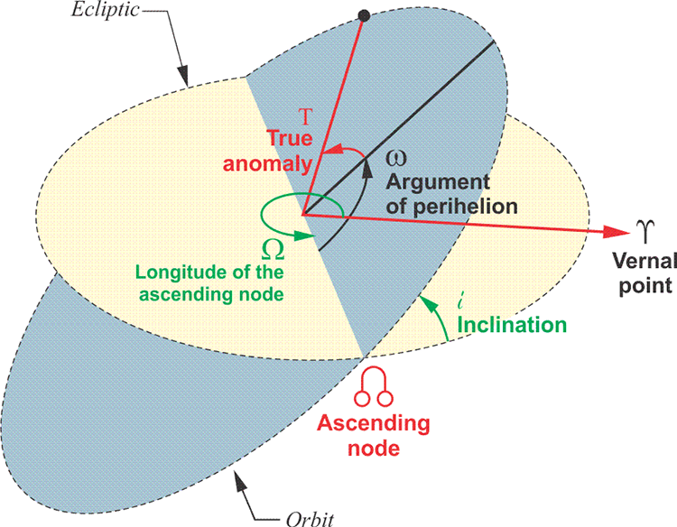
Another example of time-sensitive information is found in subframes 2 and 3 of the NAV Message. They contain information about the position of the satellite, with respect to time. This is called the satellite’s ephemeris. The ephemeris that each satellite broadcasts to the receivers provides information about its position relative to the earth. In other words, these are the coordinates of the satellite in space at the instant the Control Segment uploads the ephemerides to the Navigation Message for each individual satellite. Most particularly, it provides information about the position of the satellite antenna's phase center. The ephemeris is given in a right ascension (RA) system of coordinates. There are six orbital elements; among them are the size of the orbit, that is its semimajor axis, a, and its shape, that is the eccentricity, e. However, the orientation of the orbital plane in space is defined by other things, specifically the right ascension of its ascending node, Ω, and the inclination of its plane, i. These parameters along with the argument of the perigee, ω, and the description of the position of the satellite on the orbit, known as the true anomaly, provides all the information the user’s computer needs to calculate earth-centered, earth-fixed, World Geodetic System 1984, GPS Week 1762 (WGS84 [G1762]) coordinates of the satellite at any moment. Another example of time-sensitive information is found in subframes 2 and 3 of the Navigation message. They contain information about the position of the satellite, with respect to time. The broadcast ephemeris, however, is far from perfect. It is expressed in parameters named for the seventeenth century German astronomer Johann Kepler. The ephemerides may appear Keplerian, but in this case, the orbits of the GPS satellites deviate from nice smooth elliptical paths because they are unavoidably perturbed by gravitational and other forces. They are affected by lots of biases. Therefore, the orbits change with time so their actual paths through space are found in the result of least-squares, curve-fitting analysis. The accuracies of both the broadcast clock correction and the broadcast ephemeris deteriorate with time, so the ephemeris needs to be updated periodically to keep it within the accuracy required to get good positions on the Earth's surface. As a result, one of the most important parts of this portion of the NAV message is called IODE. IODE is an acronym that stands for Issue of Data Ephemeris, sort of a time stamp on the ephemeris that the receiver gets from the navigation message, and it appears in both subframes 2 and 3. Remember, the satellites are the control points from which the distances must be derived.
Atmospheric Correction
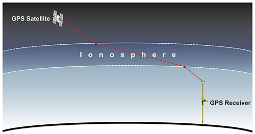
Subframe 4 addresses atmospheric correction. As with subframe 1, the data there offer only a partial solution to a problem. The Control Segment’s monitoring stations find the apparent delay of a GPS signal caused by its trip through the ionosphere through an analysis of the different propagation rates of the carrier frequencies broadcast by GPS satellites, L1, L2 and L5. These frequencies and the effects of the atmosphere on the GPS signal will be discussed later. For now, it is sufficient to say that a single-frequency receiver depends on the ionospheric correction in subframe 4 of the NAV message to help remove part of the error introduced by the atmosphere, whereas a receiver that can track more than one carrier has a bit of an advantage by comparing the differences in the frequency dependent propagation rates.
As the illustration indicates, the signal from the GPS satellite appears to slow down as it goes through the ionosphere. The atmospheric correction has been uploaded to the satellite from the Control Segment. The Control Segment can quantify the slowing because the tracking station is at a known point.
The ionosphere is dispersive. Since the GPS satellite broadcasts signals at different frequencies, it is important to understand that these frequencies are affected differently as they pass through the ionosphere. Their propagation rates are slowed differently in the ionosphere. They're not slowed at exactly the same rate. We'll talk more about that in a little bit.
For the moment, it's sufficient to say that a single frequency receiver, and there are such things, of course, a single frequency GPS receiver is somewhat handicapped by the fact that it cannot model the ionosphere. If the receiver has only one frequency to work with, it can't take advantage of the fact that it could quantify how much the signals have been affected by the ionosphere for itself, rather than relying exclusively on the Atmospheric Correction in the Navigation Message. A single frequency GPS receiver must rely almost completely on the Navigation Message Atmospheric Correction. This is a bit of a handicap. The atmosphere over Kwajalien in the Pacific might be quite different than the atmosphere above a single frequency GPS receiver in the continental US. This is one reason that the Navigation Message is not as perfect as we would like it to be.
The Almanac, Time to First Fix and Satellite Health
The Almanac
As mentioned briefly earlier, the information in the almanac in subframes 4 and 5 tells the receiver where to find all the GPS satellites. Subframe 4 contains the almanac data for satellites with pseudorandom noise (PRN) numbers from 25 through 32, and subframe 5 contains almanac data for satellites with PRN numbers from 1 through 24. The Control Segment generates and uploads a new almanac every day to each satellite, at least every six days, but typically on a daily basis.
While a GPS receiver must collect a complete ephemeris from each individual GPS satellite to know its correct orbital position, it is convenient for a receiver to be able to have some information about where all the satellites in the constellation are by reading the almanac from just one of them. The almanacs are much smaller than the ephemerides because they contain coarse orbital parameters and incomplete ephemerides, but they are still accurate enough for a receiver to generate a list of visible satellites at power-up. They, along with a stored position and time, allow a receiver to find its first satellite.
If a receiver has been in operation recently and has some leftover almanac and position data in its non-volatile memory from its last observations, it can begin its search with what is known as a warm start. A warm start is also known as a normal start. In this condition, the receiver might begin by knowing the time within about 20 seconds and its position within 100 km or so, and this approximate information helps the receiver estimate the range to satellites. For example, it will be able to restrict its search for satellites to those likely above its horizon, rather than wasting time on those below it. Limiting the range of the search decreases the time to first fix (TTFF). It can be as short as 30 seconds with a warm start.
On the other hand, if a receiver has no previous almanac or ephemeris data in its memory, it will have to perform a cold start, also known as a factory start. Without previous data to guide it, the receiver in a cold start must search for all the satellites without knowledge of its own position, velocity, or the time. When it does finally manage to acquire the signal from one, it gets some help and can begin to download an almanac. That almanac data will contain information about the approximate location of all the other satellites. The period needed to receive the full information is 12.5 minutes.
The time to first fix (TTFF) is longest at a cold start, less at warm, and least at hot. A receiver that has a current almanac, a current ephemeris, time and position can have a hot start. A hot start can take from 1/2 to 20 seconds.
Estimating how long each type of start will actually take is difficult; overhead obstructions interrupting the signal from the satellites, the GPS signals reflecting from nearby structures, etc., can delay the loading of the ephemeris necessary to lock onto the satellite's signals.
Satellite health
Subframe 1 contains information about the health of the satellite the receiver is tracking when it receives the NAV message and allows it to determine if the satellite is operating within normal parameters. Subframes 4 and 5 include health data all of the satellites, data that is periodically uploaded by the Control Segment. These subframes inform users of any satellite malfunctions before they try to use a particular signal. The codes in these bits may convey a variety of conditions. They may tell the receiver that all signals from the satellite are good and reliable, or that the receiver should not currently use the satellite because there may be tracking problems or other difficulties. They may even tell the receiver that the satellite will be out of commission in the future; perhaps it will be undergoing a scheduled orbit correction. GPS satellites' health is affected by a wide variety of breakdowns, particularly clock trouble. That is one reason they carry multiple clocks.
The almanac in sub frames four and five tell the receiver where to find the satellites. The little truncated ephemerides in the almanac help it do that. There is also information about the satellite health in the Navigation Message. GPS satellites operate in a rather hostile environment, and if they're having trouble, i.e., if some of the clocks are not operating within acceptable parameters, the health data allows the receiver to have that information. For example, a receiver might receive information that a satellite is unhealthy and shouldn't be used in the positioning.
Telemetry and Handover Words
| Subframe | 1 word | 2 words | 3-10 words |
|---|---|---|---|
| 1 | TLM | How | Clock correction, GPS week, Satellite Health, etc. |
| 2 | TLM | How | Ephemeris |
| 3 | TLM | How | Ephemeris |
| 4 | TLM | How | Ionosphere, PRN 25-32 Satellite Almanac and Health, UTC, etc. (Subframe 4 contains 25 subcommutated pages) |
| 5 | TLM | How | PRN 1-24 Satellite Almanac and Health, etc. (Subframe 5 contains 25 subcommutated pages) |
Each of these five subframes begins with the same two words: the telemetry word (TLM) and the handover word (HOW). Unlike nearly everything else in the NAV message, these two words are generated by the satellite itself. As shown in the column headed Seconds of the Week at Midnight on that Day in Table 1.1, GPS time restarts each Sunday at midnight (0:00 o’clock). These data contain the time since last restart of GPS time on the previous Sunday, 0:00 o’clock.
The TLM is the first word in each subframe. It indicates the status of uploading from the Control Segment while it is in progress and contains information about the age of the ephemeris data. It also has a constant unchanging 8-bit preamble of 10001011, and a string helps the receiver reliably find the beginning of each subframe.
The HOW provides the receiver information on the time of the GPS week (TOW) and the number of the subframe, among other things. For example, the HOW’s Z count (an internally derived 1.5 second epoch) tells the receiver exactly where the satellite stands in the generation of positioning codes.
The telemetry word indicates the status of uploading the control segment, if it's in process or not. This allows your receiver to know that.
Also, it allows you to know the beginning of each word from the data string. The handover word is useful in a couple of ways, but probably most importantly to tell your receiver where the satellite is in its broadcast of the codes. There are several codes in GPS. We will talk more about those.
The P and C/A Codes
The P and C/A codes are complicated, so complicated that they appear to be noise at first. In fact, they are known as pseudorandom noise, or PRN, codes. Actually, they are carefully designed. They have to be. They must be capable of repetition and replication. However, unlike the Navigation Message, the P and C/A codes are not vehicles for broadcasting information that has been uploaded by the Control Segment. They carry the raw data from which GPS receivers derive their time and distance measurements.
P Code
The P code is called the Precise code. It is a particular series of ones and zeroes generated at a rate of 10.23 million bits per second. It is carried on both L1 and L2, and it is very long, 37 weeks (2x1014 bits in code). Each GPS satellite is assigned a part of the P code all its own, and then repeats its portion every 7 days. This assignment of one particular week of the 37-week-long P code to each satellite helps a GPS receiver distinguish one satellite’s transmission from another. For example, if a satellite is broadcasting the fourteenth week of the P code, it must be Space Vehicle 14 (SV 14). The encrypted P code is called the P(Y) code.
There is a flag in subframe 4 of the NAV message that tells a receiver when the P code is encrypted into the P(Y) code. This security system has been activated by the Control Segment since January 1994. It is done to prevent spoofing. Spoofing is generation of false transmissions masquerading as the Precise Code. This countermeasure called Antispoofing (AS) is accomplished by the modulation of a W-Code to generate the more secure Y-Code that replaces the P code. Commercial GPS receiver manufacturers are not authorized to use the P(Y) code directly. Therefore, most have developed proprietary techniques both for carrier wave and pseudorange measurements on L2 indirectly. There is now a civilian code on L2 (L2C). There is also now a military code known as the M code. We will discuss both of these later.
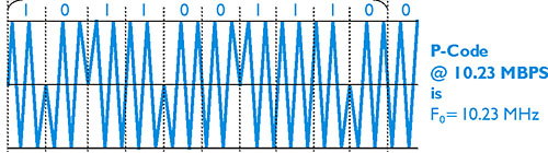
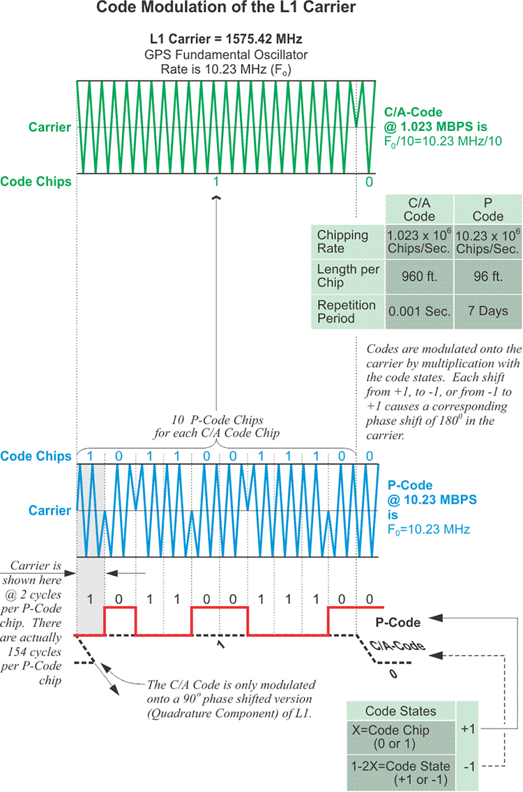
The Navigation Message can be thought of as the NAV Code, but there are others. Positioning, one of the primary objectives of GPS, is really the office of the P-Code, the C/A Code and some others that are newer than these legacy codes. The P code is the Precise code, The C/A code is the Civilian Access code. They're modulated onto carrier waves. For example, when you listen to a radio in your car and the announcer says you're listening to, let's say, 760 megahertz... well, of course, you're not listening to 760 megahertz. You can't hear that. Human hearing tops out at about 0.02 megahertz. What you hear is the modulation of speech and music onto the 760 megahertz carrier. The same idea is used in GPS. But with a radio, of course, the modulation is typically a frequency modulation or an amplitude modulation for FM and AM, respectively. In GPS, the modulation is done differently. Phase modulation is used. The image here is intending to show that. The P code in the image is a sine wave. It has particularly sharp peaks, but it is still a sine wave. Please note that up at the top of the blue line, there's a sequence of 1's and 0's. These indicate code chips of a binary code.
Please notice the way these code chips transition from 1 to 0 and back to 1. At those instances the sine wave, the blue line, does not go all the way to the top or bottom. When there is a transition from a 1 to a 0 or from a 0 to a 1, the blue line stops in the middle and reverses direction. However, when the code chip just goes from a 1 to a 1, or from a 0 to a 0, there is no interruption of the normal sine wave path. In those cases, the blue line does go all the way up to the top, and it goes all the way down to the bottom.
This technique is called phase modulation.
The C/A Code
The C/A code is also a particular series of ones and zeroes, but the rate at which it is generated is 10 times slower than the P(Y) code. The C/A code rate is 1.023 million bits per second. Here, satellite identification is quite straightforward. Not only does each GPS satellite broadcast its own completely unique 1023 bit C/A code, it repeats its C/A code every millisecond. The legacy C/A code is broadcast on L1 only. It used to be the only civilian GPS code, but no longer; it has been joined by a new civilian signal known as L2C that is carried on L2.
SPS and PPS
Still, the C/A code is the vehicle for the Standard Positioning Service, SPS, which is used for most civilian surveying applications. The P(Y) code on the other hand provides the same service for the precise positioning servicer, PPS. The idea of SPS and PPS was developed by the Department of Defense many years ago. SPS was designed to provide a minimum level of positioning capability considered consistent with national security, ±100m, 95% of the time, when intentionally degraded through Selective Availability (SA).
Selective Availability, the intentional dithering of the satellite clocks by the Department of Defense was instituted in 1989, because the accuracy of the C/A point positioning as originally rolled out was too good! As mentioned above, the accuracy was supposed to be ±100 meters horizontally, 95% of the time, with a vertical accuracy of about ±175 meters. But, in fact, it turned out that the C/A-code point positioning gave civilians access to accuracy of about ±20 meters to ±40 meters. That was not according to plan, so the satellite clocks’ accuracy was degraded on the C/A code. The good news is that the intentional error source called SA is gone. It was switched off on May 2, 2000 by presidential order. The intentional degradation of the satellite clocks is a thing of the past. Actually, Selective Availability never did hinder the surveying applications of GPS. We will delve into the reason a bit later. In any case, satellite clock errors, the unintentional kind, still contribute error to GPS positioning.
PPS is designed for higher positioning accuracy and was originally available only to users authorized by the Department of Defense; that has changed somewhat, more about that later in this chapter. It used to be that the P(Y) code was the only military code. That is no longer the case. It has been joined by a new military signal called the M-code.
The C/A Code or Civilian Acquisition or Access Code is generated 10 times slower than the P-Code. The GPS fundamental clock rate is 10.23 megahertz, but C/A Code is generated at 1.023 megabits per second.
The C/A Code is modulated onto the carrier by phase modulation, too.
The image shows a green line, a sine wave that only transitions when it reaches that center line and reverses direction. That is a phase shift, and then the code, it goes from the 1 to the 0 or from the 0 to the 1.
Modulation of Carrier Wave
All the codes mentioned come to a GPS receiver on a modulated carrier; therefore, it is important to understand how a modulated carrier is generated. The signal created by an electronic distance measuring (EDM) device in a total station is a good example of a modulated carrier.
EDM Ranging
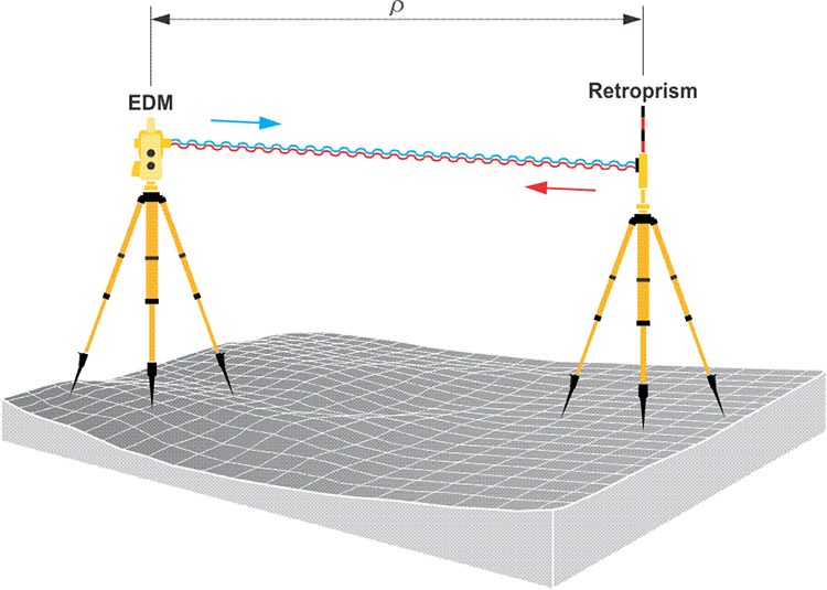
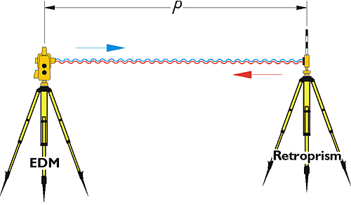
Distance measurement in modern surveying is done electronically. Distance is measured as a function of the speed of light, an electromagnetic signal of stable frequency and elapsed time. Frequencies generated within an electronic distance measuring device (EDM) can be used to determine the elapsed travel time of its signal, because the signal bounces off a reflector (aka corner cube) and returns to where it started. An EDM only needs one oscillator at the point of origin, because its electromagnetic wave travels to a retroprism and is reflected back to its origination. It is a two-way system, but the EDM is both the transmitter and the receiver of the signal. On the signal's return, the EDM can analyze it and determine the distance. In general terms, the instrument can take half the time elapsed between the moment of transmission and the moment of reception, multiply by the speed of light, and find the distance between itself and the retroprism (Distance = Elapsed Time x Rate).
The fundamental elements of the calculation of the distance measured by an EDM, ρ, are the time elapsed between transmission and reception of the signal, Δt, and the speed of light, c.
Distance = ρ
Elapsed Time = Δt
Rate = c
GPS Ranging
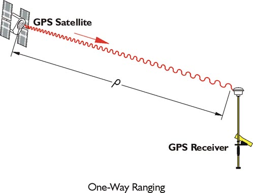
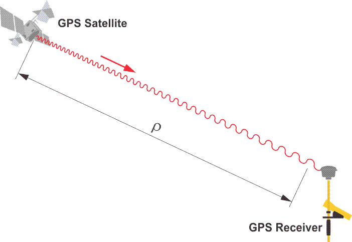
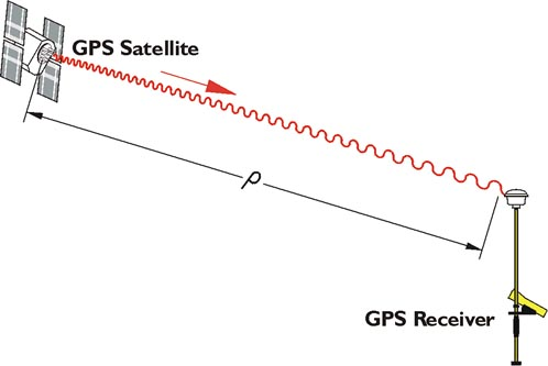
The one-way ranging used in GPS is more complicated. The broadcast signals from the satellites are collected by the receiver, not reflected. Nevertheless, the same measurement concept is used. In general terms, the full time elapsed between the instant a GPS signal leaves a satellite and arrives at a receiver, multiplied by the speed of light, is the distance between them. Unlike the wave generated by an EDM, a GPS signal cannot be analyzed at its point of origin. The measurement of the elapsed time between the signal’s transmission by the satellite and its arrival at the receiver requires two clocks (aka oscillators), one in the satellite and one in the receiver. This complication is compounded because these two clocks would need to be perfectly synchronized with one another to calculate the elapsed time, and hence the distance, between them exactly. Since such perfect synchronization is impossible, the problem is addressed mathematically.
In the image, the basis of the calculation of a range measured from a GPS receiver to the satellite, ρ, is the multiplication of the time elapsed between a signal’s transmission and reception, Δt, by the speed of light, c. A discrepancy of 1 microsecond, 1 millionth of a second, from perfect synchronization, between the clock aboard the GPS satellite and the clock in the receiver can create a range error of 299.79 meters, far beyond the acceptable limits for nearly all surveying work.
So, since perfect synchronization is not in the cards, we have to solve for time.
Phase Angles
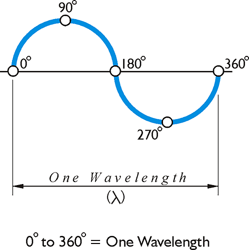
Here's a sine wave illustrating a single wavelength of 1 Hertz, that is a wavelength that takes 1 second to cycle through 360 degrees. The 0°, 90°, 180°, 270° and 360° are known as phase angles. They are important to the modulation of the carrier by phase and that is the method of attaching the codes to the GPS carriers.
The time measurement devices used in both EDM and GPS measurements are clocks only in the most general sense. They are more correctly called oscillators, or frequency standards. In other words, rather than producing a steady series of ticks, they keep time by chopping a continuous beam of electromagnetic energy at extremely regular intervals. The result is a steady series of wavelengths and the foundation of the modulated carrier. As long as the rate of an oscillator’s operation is very stable, both the length and elapsed time between the beginning and end of every wavelength of the modulation will be the same. Therefore, the phase angles will also occur at definite and constant distances.
Phase Shift
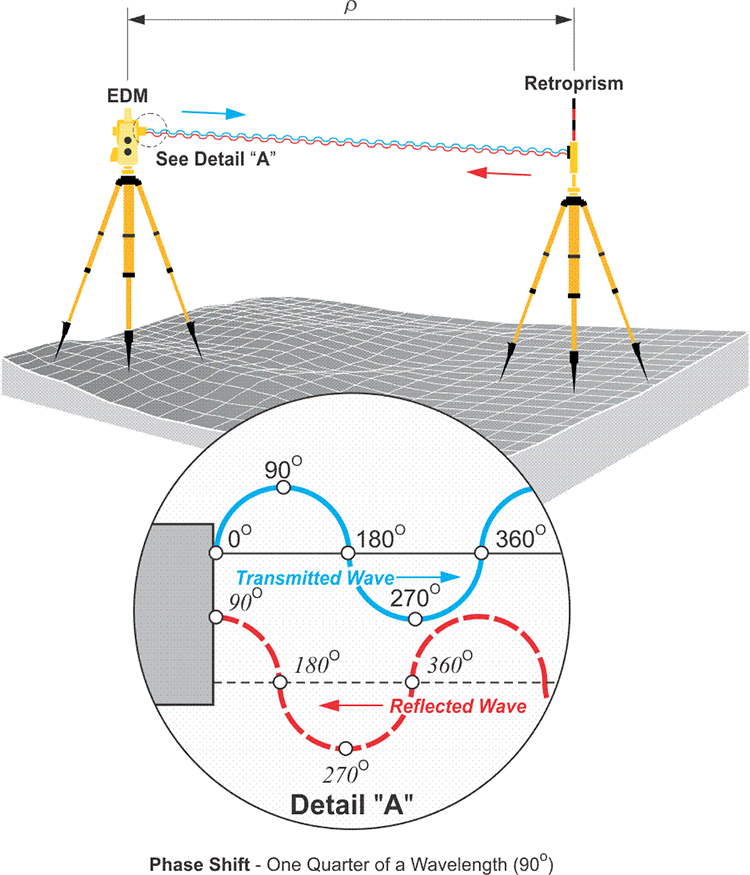
Phase Shift
The image shows again the EDM sending out the transmitted wave in blue, with the phase angles indicated as before. The signal goes to the retro prism and returns. When it returns, shown in the dashed red line, notice the phase angles. It is clear that the return signal does not come back exactly in phase with the transmitted wave. In other words, the phase angles on the reflected wave do not match those on the transmitted wave. The key element here is that the EDM generates another wave that is exactly the same as the wave it transmitted. However, it keeps the additional wave (the blue one) at home so that when the reflected wave returns, it can be compared with it. By comparing the returned wave—the one here in the dashed red line—with the exact replica of the transmitted wave, the EDM can determine how much the returned wave is phase shifted, that is out of phase, with the original transmitted wave.
Since all measurements will not neatly fit complete wavelengths, the EDM finds the fractional part of its measurement electronically. It does a comparison. It compares the phase angle of the returning signal to that of a replica of the transmitted signal that it keeps inside to determine the phase shift. That phase shift represents the fractional part of the measurement.
How does it work? First, it is important to remember that points on a modulated carrier are defined by phase angles, such as 0°, 90°, 180°, 270° and 360°. When two modulated carrier waves reach exactly the same phase angle at exactly the same time, they are said to be in phase, coherent, or phase locked. However, when two waves reach a phase angle at different times, they are out of phase or phase shifted. For example, in the image, the sine wave shown by the dashed red line has returned to an EDM from a reflector. Compared with the sine wave shown by the solid blue line, it is out of phase by one-quarter of a wavelength. The distance between the EDM and the reflector, ρ, is then:
where:
N = the number of full wavelengths the modulated carrier has completed
d = the fractional part of a wavelength at the end that completes the doubled distance.
In this example, d is three-quarters of a wavelength because it lacks its last quarter.
Both EDM and GPS ranging use the method represented in this illustration. In GPS, the measurement of the difference in the phase of the incoming signal and the phase of the internal oscillator in the receiver reveals the small distance at the end of a range. In GPS, the process is called carrier phase ranging, as the name implies, the observable is the carrier wave itself in that case.
The Integer Ambiguity Problem
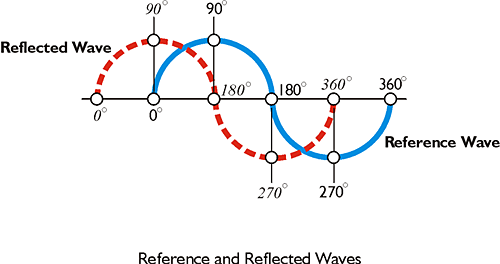
Both EDM and GPS ranging use the method represented in this illustration. In GPS, the measurement of the difference in the phase of the incoming signal and the phase of the internal oscillator in the receiver reveals the small distance at the end of a range.
By comparing the phase of the signal returned from the reflector with the reference wave it kept at home, an EDM can measure how much the two are out of phase with one another. However, this measurement can only be used to calculate a small part of the overall distance. It only discloses the length of a fractional part of a wavelength used. This leaves a big unknown, namely the number of full wavelengths of the EDM’s modulated carrier between the transmitter and the receiver at the instant of the measurement. This cycle ambiguity is symbolized by N. Fortunately, the cycle ambiguity can be solved in the EDM measurement process. The key is using carriers with progressively longer wavelengths. For example, the submeter portion of the overall distance can be resolved using a carrier with the wavelength of a meter. This can be followed by a carrier with a wavelength of 10 meters, which provides the basis for resolving the meter aspect of a measured distance. This procedure may be followed by the resolution of the tens of meters using a wavelength of 100 meters. The hundreds of meters can then be resolved with a wavelength of 1000 meters, and so on.
Here is that comparison, the reference wave in blue with the reflected wave with the dashed red line. The reflected wave came back out of phase by a quarter of a wavelength. With an EDM, wavelengths of varying length can be sent out. For example, if the EDM sends out a wavelength of 100 meters, then by looking at the fractional part of that 100-meter wavelength, it would be possible to determine the tens of meters in the distance. The hundreds of meters of the overall distance could be resolved by sending out a wavelength of 1,000 meters and looking at the fractional part (by phase comparison). This method depends on the fact that the EDM survey can send out waves of different wavelengths and have them return to where they came from. That makes comparison of the returned wave with the reference wave possible. By comparing phase angles, the fractional part of the wavelength that went out can be determined. The components of the total distance are built up by sending on wavelengths of different size; first the thousands of feet, then the hundreds of feet, then the single feet, and finally the decimals of feet. However, this whole method is not possible in GPS surveying. There are only three carriers; L1, L2, and L5. They have constant wavelengths. Therefore, while it's possible to determine the fractional part of the wavelength, that one small component of the distance, from a single measurement, knowing the number of full wavelengths between the receiver and satellite is more difficult. This is known as the integer ambiguity problem.
A Different Strategy
Unlike an EDM measurement, the wavelengths of GPS carriers cannot be periodically changed to resolve the cycle ambiguity problem. GPS needs a different strategy. The satellites broadcast only three carriers, L1, L2 and L5. They have constant wavelengths and only propagate from the satellites to the receivers, one direction. Still, the carrier phase measurements remain an important observable in GPS ranging.
Two Types of Observables

The word observable is used throughout GPS literature to indicate the signals whose measurement yields the range or distance between the satellite and the receiver. The word is used to draw a distinction between the thing being measured, "the observable" and the measurement, "the observation." In GPS, there are two types of observables. The codes are one type of observable. We've talked about how that is modulated onto the carrier. There's another type of observable. That's the carrier itself without the codes. The carrier is the basis of the techniques used for high-precision GPS surveys. In the upper image, you see the pseudorange code observable illustrated as square waves of code states, and in the lower image, you see the carrier wave observable, which is just a constant sine wave, not modulated. The code solution provides a pseudorange. The pseudorange can serve applications when virtually instantaneous point positions are required or relatively low accuracy will suffice. These basic observables can also be combined in various ways to generate additional measurements that have certain advantages. It is in this latter context that pseudoranges are used in many GPS receivers as a preliminary step toward the final determination of position by a carrier phase measurement. Many GPS receivers use the pseudorange code observable as sort of the front door, a way to begin the determination of a position, and then, frequently, they switch to the carrier to refine that position. The foundation of pseudoranges is the correlation of code carried on a modulated carrier wave received from a GPS satellite with a replica of that same code generated in the receiver. Most of the GPS receivers used for surveying applications are capable of code correlation. That is, they can determine pseudoranges. These same receivers are usually capable of determining ranges using the unmodulated carrier, as well. However, first let us concentrate on the pseudorange.
Spread Spectrum and Code Modulation of L1 GPS Carrier
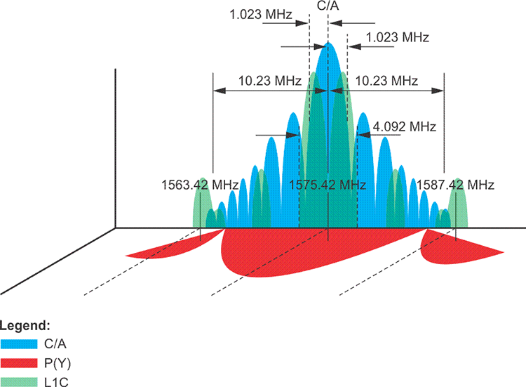
A carrier wave can be modulated in various ways. Radio stations use modulated carrier waves. The radio signals are AM, amplitude modulated or FM, frequency modulated. When your radio is tuned to 105 FM, you are not actually listening to 105 MHz; despite the announcer’s assurances, it is well above the range of human hearing. 105 MHz is just the frequency of the carrier wave that is being modulated. It is those modulations that occur that make the speech and music intelligible. They come to you at a much slower frequency than does the carrier wave. The GPS carriers L1, L2, and L5 could have been modulated in a variety of ways to carry the binary codes, the 0s and 1s, that are the codes. Neither amplitude nor frequency modulation are used in GPS. It is the alteration of the phases of the carrier waves that encodes them. It is phase modulation that allows them to carry the codes from the satellites to the receivers. One consequence of this method of modulation is that the signal can occupy a broader bandwidth than would otherwise be possible. The GPS signal is said to have a spread spectrum because of its intentionally increased bandwidth. In other words, the overall bandwidth of the GPS signal is much wider than the bandwidth of the information it is carrying. In other words, while L1 is centered on 1575.42 MHz, L2 is centered on 1227.60 MHz, and L5 on 1176.45 MHz, but the width of these signals takes up a good deal more space on each side of these frequencies than might be expected. For example, the C/A code signal is spread over a width of 2.046 MHz or so, the P(Y) code signal is spread over a width about 20.46 MHz on L1 and the coming L1C signal will be spread over 4.092 MHz as shown in the image above.
This characteristic offers several advantages. It affords better signal to noise ratio, more accurate ranging, less interference, and increased security. However, spreading the spectral density of the signal also reduces its power. The weakness of the signal makes it difficult to receive undercover.
In any case, the most commonly used spread spectrum modulation technique is known as binary phase shift keying (BPSK). This is the technique used to create the NAV Message, the P(Y) code and the C/A code. The binary biphase modulation is the switching from 0 to 1 and from 1 to 0 accomplished by phase changes of 180º in the carrier wave. Put another way, at the moments when the value of the code must change from 0 to 1, or from 1 to 0, the change is accomplished by an instantaneous reverse of the phase of the carrier wave. It is flipped 180º. And each one of these flips occurs when the phase of the carrier is at the zero-crossing (the gray centerline inthe middle of the sine wave illustrations above). Each 0 and 1 of the binary code is known as a code chip. 0 represents the normal state, and 1 represents the mirror image state.
The rate of all of the components of GPS signals are multiples of the standard rate of the oscillators. The standard rate is 10.23 MHz. It is known as the fundamental clock rate and is symbolized Fo For example, the GPS carriers are 154 times Fo, or 1575.42 MHz, 120 times Fo, or 1227.60 MHZ, and 115 times Fo, or 1176.45 MHZ. These represent L1, L2, and L5 respectively. The codes are also based on Fo. 10.23 code chips of the P(Y) code, 0s or 1s, occur every microsecond. In other words, the chipping rate of the P(Y) code is 10.23 million bits per second (Mbps), exactly the same as Fo, 10.23 MHZ. The chipping rate of the C/A code is 10 times slower than the P(Y) code. It is one tenth of Fo, 1.023 Mbps. Ten P(Y) code chips occur in the time it takes to generate one C/A code chip. This is a reason why a P(Y) code derived pseudorange is more precise than a C/A code pseudorange.
More About Code Chips
Up at the top is the C/A Code in the green and the P-Code is in the blue below it. There are several pieces of information here. One of the things you might notice right away is the red square wave from 1 to 0 and 0 to 1 indicated down at the bottom.
For each 180-degree phase shift, there's this shift from the 1 to the 0 and back to 1, and this is represented by this red square wave. See that the C/A Code is also represented by the dashed black square wave that is turned 90 degrees or in quadrature to the P-Code.
If there were no shift in the phase of the carriers, they would not be modulated and would not be carrying the codes.
The codes chipping rates are shown on the right-hand side. Please notice that the C/A Code chipping rate is 10 times slower than the P-Code.
L1 is broadcast at 1575.42 megahertz. Its rate is a multiple of the fundamental clock rate of 10.23 megahertz.
The length of a C/A Code is 960 feet, whereas, the length of a P-Code, 10 times shorter, because the P-Code is 10 times faster, is 96 feet, and also notice the repetition period. You see here, also, the 10 P-Codes per each C/A Code chip, which is exactly as you would expect.
The C/A Code is repeated very quickly; whereas the P-Code does not repeat for seven days, making it more secure as would be expected with a classified precise code.
Code Correlation
Strictly speaking, a pseudorange observable is based on a time shift. This time shift can be symbolized by dτ, d tau, and is the time elapsed between the instant a GPS signal leaves a satellite and the instant it arrives at a receiver. The concept can be illustrated by the process of setting a watch from a time signal heard over a telephone.
Propagation Delay
Imagine that a recorded voice said, “The time at the tone is 3 hours and 59 minutes.” If a watch was set at the instant the tone was heard, the watch would be wrong. Supposing that the moment the tone was broadcast was indeed 3 hours and 59 minutes, the moment the tone is heard must be a bit later. It is later because it includes the time it took the tone to travel through the telephone lines from the point of broadcast to the point of reception. This elapsed time would be approximately equal to the length of the circuitry traveled by the tone divided by the speed of the electricity, which is the same as the speed of all electromagnetic energy, including light and radio signals. In fact, it is possible to imagine measuring the actual length of that circuitry by doing the division.
In GPS, that elapsed time is known as the propagation delay, and it is used to measure length. The measurement is accomplished by a combination of codes. The idea is somewhat similar to the strategy used in EDMs. But where an EDM generates an internal replica of its carrier wave to correlate with the signal it receives by reflection, a pseudorange is measured by a GPS receiver using a replica of a portion of the code that is modulated onto the carrier wave. The GPS receiver generates this replica itself and it is used to compare with the code that is coming in from the satellite.
Code Correlation
To conceptualize the process, one can imagine two codes generated at precisely the same time and identical in every regard: one in the satellite and one in the receiver. The satellite sends its code to the receiver but, on its arrival, the codes do not line up even though they are identical. They do not correlate, that is, until the replica code in the receiver is time shifted a little bit. Once that is done, the receiver generated replica code fits the received satellite code. It is this time shift that reveals the propagation delay. The propagation delay is the time it took the signal to make the trip from the satellite to the receiver, dτ. It is the same idea described above as the time it took the tone to travel through the telephone lines, except the GPS code is traveling through space and atmosphere. Once the time shift of the replica code is accomplished, the two codes match perfectly and the time the satellite signal spends in transit has been measured, well, almost. It would be wonderful if that time shift could simply be divided by the speed of light and yield the true distance between the satellite and the receiver at that instant, and it is close, but there are physical limitations on the process that prevent such a perfect relationship.
Autocorrelation
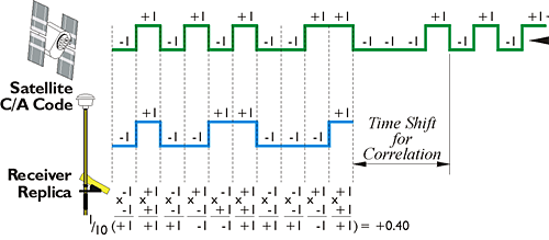
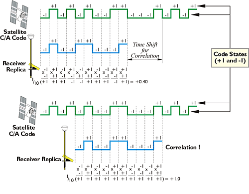
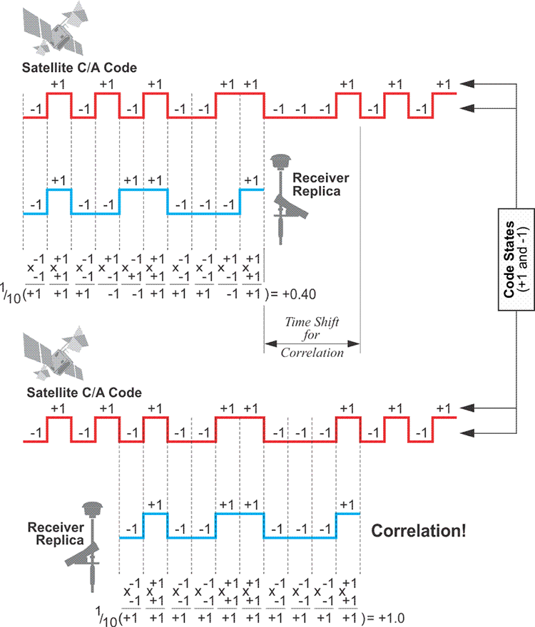
As mentioned earlier, the almanac information from the NAV message of the first satellite a GPS receiver acquires tells it which satellites can be expected to come into view. With this information, the receiver can load up pieces of the C/A codes for each of those satellites. Then the receiver tries to line up the replica C/A codes with the signals it is actually receiving from the satellites. Actually lining up the code from the satellite with the replica in the GPS receiver is called autocorrelation, and depends on the transformation of code chips into code states. The formula used to derive code states (+1 and -1) from code chips (0 and 1) is:
code state = 1-2x
where x is the code chip value. For example, a normal code state is +1, and corresponds to a code chip value of 0. A mirror code state is -1, and corresponds to a code chip value of 1.
The function of these code states can be illustrated by asking three questions: First, if a tracking loop of code states generated in a receiver does not match code states received from the satellite, how does the receiver know? In that case, for example, the sum of the products of each of the receiver’s 10 code states, with each of the code states from the satellite, when divided by 10, does not equal 1. In the example in the illustration, the result is 0.40. Second, what does the receiver do when the code states in the receiver do not match the code states received from the satellite? It shifts the frequency of its search a little bit from the center of the L1 1575.42 MHZ. This is done to accommodate the inevitable Doppler shift of the incoming signal, since the satellite is always either moving toward or away from the receiver. The receiver also shifts its piece of code in time. These iterative small shifts in both time and frequency continue until the receiver code states do in fact match the signal from the satellite. Third, how does the receiver know when a tracking loop of replica code states does match code states from the satellite? In the case illustrated in the image, the sum of the products of each code state of the receiver’s replica 10, with each of the 10 from the satellite, divided by 10, is exactly 1. This is shown in the illustration at "Correlation!" where the receiver’s replica code fits the code from the satellite like a key fits a lock.
The interesting thing is that that time shift for correlation gives the receiver approximately the amount of elapsed time that it took the signal to come from the satellite to the receiver. Obviously, if the receiver knows the elapsed time, and it knows the frequency of the signal, it then knows the distance (the range) between itself and the satellite. This is how the pseudorange works. If this were the whole story, we'd be done, and of course, it isn't the whole story.
The Delay Lock Loop
Once correlation of the two codes is achieved with a delay lock loop (DLL), it is maintained by a correlation channel within the GPS receiver, and the receiver is sometimes said to have achieved lock or to be locked on to the satellites. The receiver can continue to log the signal from the satellite and stay correlated unless it is somehow interrupted by a cycle slip or an obstruction. If that happens, the receiver is said to have lost lock. However, as long as the lock is present, the NAV message is available to the receiver. Remember that one of its elements is the broadcast clock correction that relates the satellite's on board clock to GPS time, and a limitation of the pseudorange process comes up.
Imperfect Oscillators and Clock Corrections
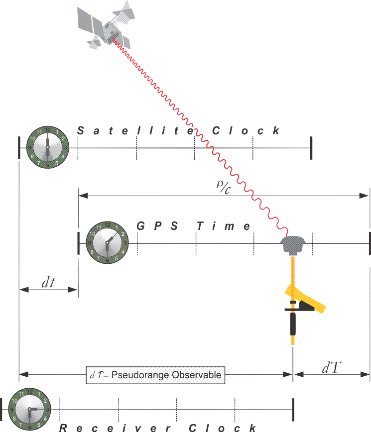
One reason the time shift, dτ (d tau), found in autocorrelation cannot quite reveal the true range, ρ, of the satellite at a particular instant is the lack of perfect synchronization between the clock in the satellite and the clock in the receiver. Recall that the two compared codes are generated directly from the fundamental rate, Fo, of those clocks. And since these widely separated clocks, one on Earth and one in space, cannot be in perfect lockstep with one another, the codes they generate cannot be in perfect sync either. Therefore, a part of the observed time shift, dτ (d tau), must always include the disagreement between these two clocks. In other words, the time shift not only contains the signal’s transit time from the satellite to the receiver, it contains clock errors, and other errors too. In fact, whenever satellite clocks and receiver clocks are checked against the carefully controlled GPS time, they are found to be drifting a bit. Their oscillators are imperfect. It is not surprising that they are not quite as stable as the atomic clocks around the world that are used to define the rate of GPS time. They are subject to the destabilizing effects of temperature, acceleration, radiation, and other inconsistencies. In other words, clock offsets bias every satellite to receiver pseudorange observable. The difference between the satellite clock's time and GPS time is shown in dt (d small t) in the illustration. The difference in the receiver's clock from GPS time is shown in dT (d capital T) in the illustration. While the pseudorange observable shown here in dτ (d tau) is intended to be the amount of time that it took the signal to reach the receiver from the satellite, there are some difficulties. Among them are the fact that the receiver's clock is probably a quartz oscillator, and it's not terribly stable, and the clock correction in the Navigation Message which was uploaded some time before it is received isn't exactly right either. Such discrepancies are important when a nanosecond, a billionth of a second, is approximately a foot. Therefore, the pseudorange has some errors that are difficult to remove. The pseudorange, by itself, while it has the virtue of being approximately correct, is certainly not at the level of accuracy that we have come to expect from GPS. That is one reason it is called a pseudorange (i.e. false range)
The Pseudorange Equation

Clock offsets are only one of the errors in pseudoranges. Please note that the pseudorange, p, and the true range, ρ, cannot be made equivalent without consideration of clock offsets, atmospheric effects and other biases that are inevitably present.
Some of those errors are shown in this equation. On the left-hand side, the pseudorange measurement equals rho, the true range, plus all of these other factors. If it were correct initially, if the pseudorange was good and complete by itself, these other factors would not need to be considered. The pseudorange, p, would be equal to the true range, rho. But, in fact, there are satellite orbital errors because the orbits of the satellites are affected by many factors including the variations in gravity, drag, and tidal forces from the sun, the moon, etc. The speed of light is constant in a vacuum, but it has to be multiplied times the satellite clock offset from GPS time minus the receiver clock offset from GPS time, because of propagation delay and imperfect oscillators among other things. While the satellite clock offset from GPS time is somewhat known from the Navigation Message, it's not perfectly known. The receiver clock offset from GPS time is not well known at all. Then, there is the ionospheric delay to be considered. There's also a bit of tropospheric delay. The troposphere includes the atmospheric layers below the ionosphere.
Then, on top of that, there's something known as multipath. Multipath means that the signal from the GPS satellite bounces off of something before it gets into the receiver. Obviously, if you're measuring distances to determine your position, that bounce creates a difficulty. There is receiver noise as a bias in the system. This is like the static that can appear on your car radio.
In short, all these biases contaminate the pseudorange position. So, while the pseudorange is a good way to get started with a GPS position, it isn't the full answer.
The One-percent Rule of Thumb

Here is convenient approximation. The maximum resolution available in a pseudorange is about 1 percent of the chipping rate of the code used. It offers a basis to evaluate pseudoranging in general and compare the potentials of P(Y) code and C/A code pseudoranging in particular. A P(Y) code chip occurs every 0.0978 of a microsecond. In other words, there is a P(Y) code chip about every tenth of a microsecond. That’s one code chip every 100 nanoseconds. Therefore, a P(Y) code based measurement can have a maximum precision of about 1 percent of 100 nanoseconds, or 1 nanosecond. What is the length of 1 nanosecond? Well, multiplied by the speed of light, it's approximately 30 centimeters, or about a foot. So, just about the very best you can do with a P(Y) pseudorange is a foot or so. Because its chipping rate is 10 times slower, the C/A code based pseudorange is 10 times less precise. Therefore, one percent of the length of a C/A code chip is 10 times 30 centimeters, or 3 meters. Using the rule of thumb, the resolution of a C/A code pseudorange is nearly 10 feet.
You might ask, at this point, if the pseudorange isn't the full answer, then how do we get the extraordinary accuracies that we depend upon GPS to produce?
The Carrier Phase Observable
This same 1 percent rule of thumb can illustrate the increased precision of the carrier phase observable over the pseudorange. First, the length of a single wavelength of each carrier is calculated using this formula
where:
= the length of each complete wavelength in meters;
= the speed of light corrected for atmospheric effects;
= the frequency in hertz.
L1 – 1575.42 MHz carrier transmitted by GPS satellites has a wavelength of approximately 19 cm
L2 – 1227.60 MHz carrier transmitted by GPS satellites has a wavelength of approximately 24 cm
The resolution available from a signal is approximately 1% of its wavelength. 1% of these wavelengths is approximately 2mm.
Carrier phase observations are certainly the preferred method for the higher precision work most have come to expect from GPS.
Discussion
Discussion Instructions
To begin the discussion sparked by the material in this lesson, I would like to pose this question:
There are both similarities and differences between a GPS carrier phase observation and a distance measurement by an EDM. Can you describe a few of each?
To participate in the discussion, please go to the Lesson 1 Discussion Forum in Canvas. (That forum can be accessed at any time by going to the GEOG 862 course in Canvas and then looking inside the Lesson 1 module.)
Summary
Now that you have some ideas about how the GPS signal carries information from the satellites to the receivers, you can delve into the errors that affect that information. The complete carrier phase observable equation can be stated as:
On the left side of the equation is the complete raw range measurement from the satellite to the receiver. On the right side is the correct range between the two and several errors known as biases.
The next lesson will give you an idea of both the origins and magnitudes of those biases.
Before you go on to Lesson 2, double-check the Lesson 1 Checklist to make sure you have completed all of the activities listed there.