Lesson 6: State Plane Coordinates and Heights
The links below provide an outline of the material for this lesson. Be sure to carefully read through the entire lesson before returning to Canvas to submit your assignments.
Lesson 6 Overview
Overview
In the opening sentence of my book Basic GIS Coordinates, “Coordinates are slippery devils. A stake driven into the ground holds a clear position, but it is awfully hard for its coordinates to be so certain, even if the figures are precise.” I try to give the sense that coordinate systems must and do evolve as measurement technology improves. That has certainly been the case with the advent of GPS/GNSS. That is reflected in the commonly used systems of State Plane Coordinates and also in heights. It may come as a bit of surprise, but the height, or elevation, that is most easily derived from satellite positioning is almost certainly not the sort of height you are after. Also, did you know that the string of a plumb bob is actually very slightly curved? We will discuss these issues and the concepts at their foundation.
Objectives
At the successful completion of this lesson, students should be able to:
- explain the basics of State Plane Coordinates;
- describe NAD83 positions and plane coordinates;
- identify map projections;
- define map distortion;
- differentiate between SPCS27 and SPCS83;
- describe scale and distance in State Plane Coordinates;
- explain the basics of heights;
- identify ellipsoidal heights;
- recognize orthometric heights;
- discuss the evolution of the vertical datum in North America; and
- recognize the geoid.
Questions?
If you have any questions now or at any point during this week, please feel free to post them to the Lesson 6 Discussion Forum. (To access the forum, return to Canvas and navigate to the Lesson 6 Discussion Forum in the Lesson 6 module.) While you are there, feel free to post your own responses if you, too, are able to help out a classmate.
Checklist
Lesson 6 is one week in length. (See the Calendar in Canvas for specific due dates.) To finish this lesson, you must complete the activities listed below. You may find it useful to print this page out first so that you can follow along with the directions.
| Step | Activity | Access/Directions |
|---|---|---|
| 1 | Read the lesson Overview and Checklist. | You are in the Lesson 6 online content now. The Overview page is previous to this page, and you are on the Checklist page right now. |
| 2 | Read "State Plane Coordinates" and "Heights" in Chapter 5- pages 140 to 170 in GPS for Land Surveyors. | Text |
| 3 | Read the lecture material for this lesson. | You are currently on the Checklist page. Click on the links at the bottom of the page to continue to the next page, to return to the previous page, or to go to the top of the lesson. You can also navigate the lecture material via the links in the Lessons menu. |
| 4 | Participate in the Discussion. | To participate in the discussion, please go to the Lesson 6 Discussion Forum in Canvas. (That forum can be accessed at any time by going to the GEOG 862 course in Canvas and then looking inside the Lesson 6 module.) |
| 5 | Take the Lesson 6 Quiz (this quiz will cover Lessons 1, 2, 3, 4, 5, and 6). | The Lesson 6 Quiz is located in the Lesson 6 module in Canvas. |
| 6 | Read lesson Summary. | You are in the Lesson 6 online content now. Click on the "Next Page" link to access the Summary. |
State Plane Coordinates
Welcome to Lesson Six of this GPS/GNSS course. And this time, we'll be talking about two coordinate systems. And I have a little bit of discussion concerning heights. We've touched on that a little bit. Now these coordinate systems that we're going to discuss are plane coordinate systems based upon the fiction that the earth is flat, which, of course, immediately introduces distortion. However, much of GIS work—and GPS/GNSS work as well—is done based upon this presumption. So, it is worthwhile to spend some time discussing how the distortions are handled and some of the elements. So, we will be talking about State Plane coordinates and Universal Transverse Mercator coordinates, both plane coordinate systems. And we'll be discussing ellipsoidal heights, and geoidal heights, and orthometric heights.
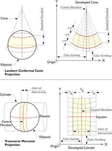
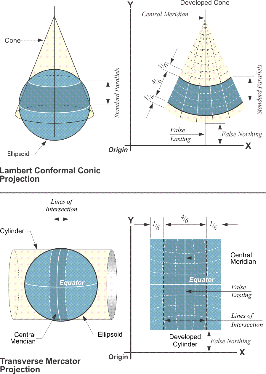
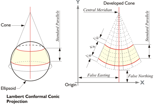
In the illustration, the Lambert conformal conic projection is on the top and the Transverse Mercator projection is on the bottom.
These plane coordinates, both State Plane and UTM, are far from an anachronism. The UTM projection has been adopted by the IUGG, the same organization that reached the international agreement to use GRS80 as the reference ellipsoid for the modern geocentric datum. NATO and other military and civilian organizations worldwide also use UTM coordinates for various mapping needs. UTM coordinates are often useful to those planning work that embraces large areas. In the United States, State Plane systems based on the Transverse Mercator projection, an Oblique Mercator projection, and the Lambert Conic map projection, grid every state, Puerto Rico, and the U.S. Virgin Islands into their own plane rectangular coordinate system. And GPS/GNSS surveys performed for local projects and mapping are frequently reported in the plane coordinates of one of these systems. State Plane Coordinates rely on an imaginary flat reference surface with Cartesian axes. They describe measured positions by ordered pairs, expressed in northings and eastings, or y- and x- coordinates. The y coordinate is the northing and the x coordinate is the easting. Despite the fact that the assumption of a flat Earth is fundamentally wrong, calculation of areas, angles and lengths using latitude and longitude can be complicated, so plane coordinates persist because they are convenient. The calculations can be done with plane trigonometry. GIS coordinate systems typically are plane. As long as the extent of the coverage of the coordinate system is limited, the curvature aspect—while it leads to distortion—can be managed. It's when the flat map, the flat coordinate system, extends beyond a limited area that the distortion can get out of hand. Therefore, the projection of points from the Earth’s surface onto a reference ellipsoid and finally onto flat maps is still viable.
Map Projection
State Plane Coordinate Systems are built on map projections. Map projection means representing a portion of the actual Earth on a plane. Done for hundreds of years to create paper maps, it continues, but map projection today is most often really a mathematical procedure done in a computer. Nevertheless, even in an electronic world, it cannot be done without distortion.

Orange Peel
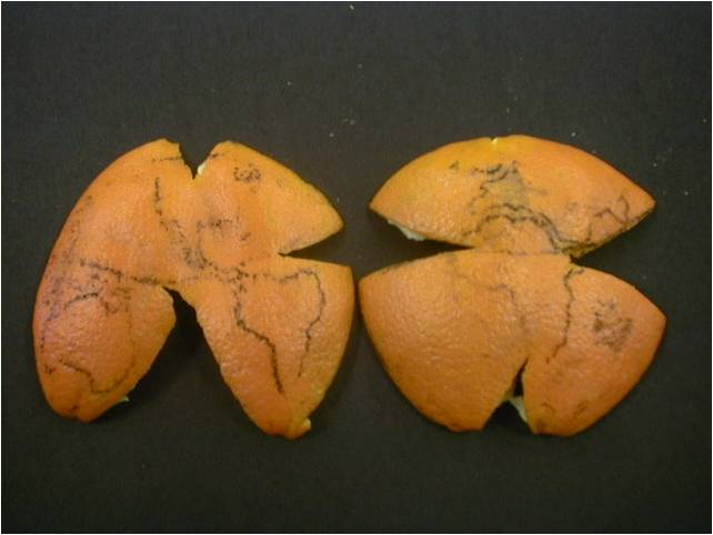
The problem is often illustrated by trying to flatten part of an orange peel. The orange peel stands in for the surface of the earth. A small part can be pushed flat without much noticeable deformation.
Distortion
However, when the portion of the orange peel gets larger, problems appear. Suppose the whole orange peel is involved; as the center is pushed down, the edges tear or stretch, or both. And if the peel gets even bigger, the tearing gets more severe. So, if a map is drawn on the orange before it is peeled, the map gets distorted in unpredictable ways when it is flattened. And it is difficult to relate a point on one torn piece with a point on another in any meaningful way.
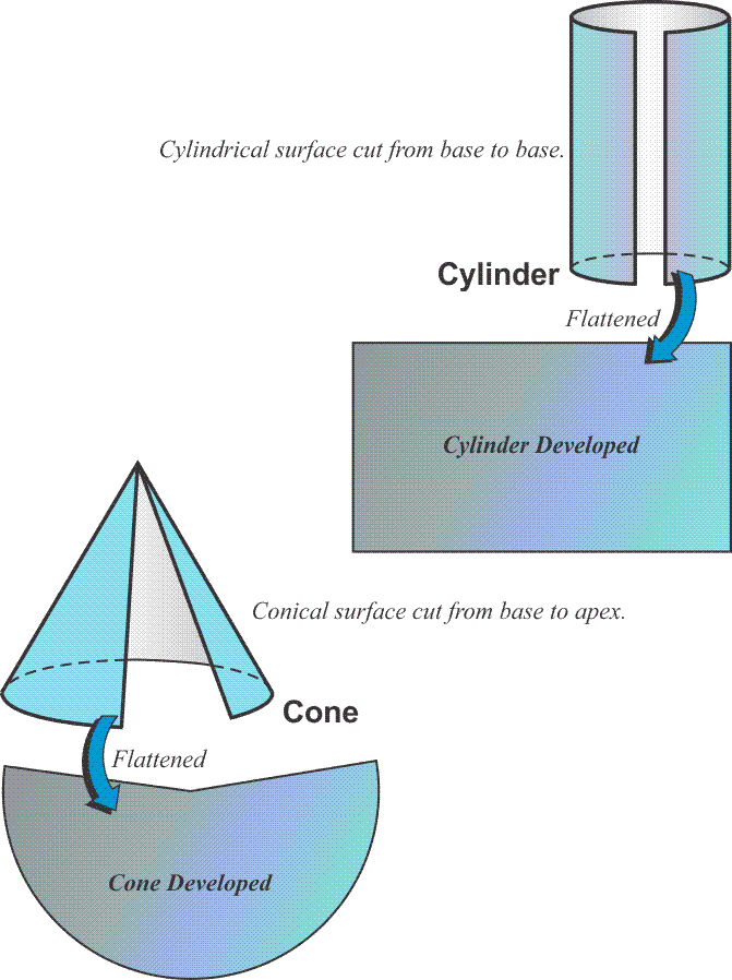
These are the problems that a map projection needs to solve to be useful. The first problem is the surface of an ellipsoid, like the orange peel, is non-developable. In other words, flattening it inevitably leads to distortion. So, a useful map projection ought to start with a surface that is developable, a surface that may be flattened without all that unpredictable deformation. It happens that a paper cone or cylinder both illustrate this idea nicely. They are illustrations only, models for thinking about the issues involved. If a right circular cone is cut perpendicularly from the base to its apex, the cone can then be made completely flat without trouble. The same may be said of a cylinder cut perpendicularly from base to base. A developable surface can be split up an element and flattened as you see in the two illustrated developable surfaces, a cylinder and a cone shown in the figure above. The cylinder is used in Mercator and Transverse Mercator map projections, and the cone is used in Lambert Conic map projections. These include the two that are most common in State Plate coordinate systems. There is one oblique portion of State Planes along the panhandle of Alaska. The right circular cone, if cut up one of its elements that is perpendicular from the base to the apex, can be completely flattened without trouble. And the same can be said of a cylinder cut up perpendicular from base to base.
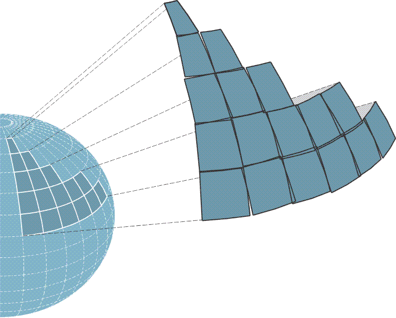
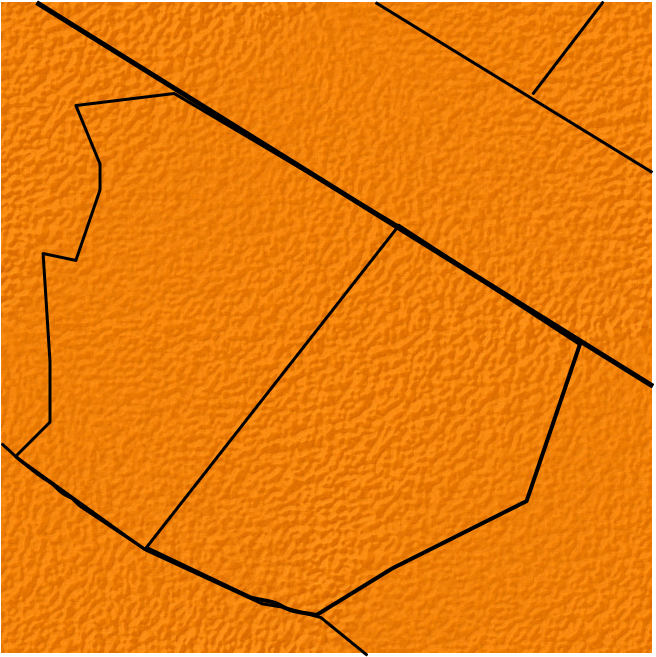
Or one could use the simplest case, a surface that is already developed. A flat piece of paper is an example. If the center of a flat plane is brought tangent to the earth, a portion of the planet can be mapped on it, that is, it can be projected directly onto the flat plane. In fact, this is the typical method for establishing an independent local coordinate system. These simple Cartesian systems are convenient and satisfy the needs of small projects. The method of projection, onto a simple flat plane, is based on the idea that a small section of the earth, as with a small section of the orange mentioned previously, conforms so nearly to a plane that distortion on such a system is negligible. Subsequently, local tangent planes have been long used. Such systems demand little if any manipulation of the field observations, and the approach has merit as long as the extent of the work is small. It's convenient. It's easy. It can satisfy small projects fairly well, but the larger each of the planes grows, the more untenable it becomes. Another difficulty arises when the local coordinate systems are brought together—as you see in this image—they simply don't match. There are overlaps, there are gaps. The scale of each of the local systems are not the same, nor is their orientation. In other words, a local tangent coordinate system can be useful in a very limited extent, as long as one stays within the zone that it intends to cover. When you bring in another coordinate system from another direction, trouble ensues. So as the area being mapped grows, the reduction of observations becomes more complicated and must take account of the actual shape of the earth. This usually involves the ellipsoid, the geoid, and geographical coordinates, latitude and longitude. At that point, surveyors and engineers rely on map projections to mitigate the situation and limit the now troublesome distortion. This is one of the reasons State Plane coordinate systems were devised. A well-designed map projection can offer the convenience of working in plane Cartesian coordinates and while not eliminating the inevitable distortion keep it at manageable levels. They cover an entire state or a fairly good portion of the state with a zone or zones.
Distortion
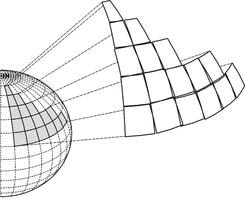
Here is a bit more on that idea. The design of local tangent plane projections must accommodate some awkward facts. For example, while it would be possible to imagine mapping a considerable portion of the earth using a large number of small individual planes, like facets of a gem, it is seldom done because when these planes are brought together they cannot be edge-matched accurately. They cannot be joined properly along their borders. And the problem is unavoidable because the planes, tangent at their centers, inevitably depart more and more from the reference ellipsoid at their edges, and the greater the distance between the ellipsoidal surface and the surface of the map on which it is represented, the greater the distortion on the resulting flat map. This is true of all methods of map projection. Therefore, one is faced with the daunting task of joining together a mosaic of individual maps along their edges where the accuracy of the representation is at its worst, and even if one could overcome the problem by making the distortion, however large, the same on two adjoining maps, another difficulty would remain. Typically, each of these planes has a unique coordinate system. The orientation of the axes, the scale, and the rotation of each one of these individual local systems will not be the same as those elements of its neighbor’s coordinate system. Subsequently, there are gaps and overlaps between adjacent maps, and their attendant coordinate systems, because there is no common reference system. Even if it was possible to accommodate, let's say, a GIS coordinate system with a local coordinate system, it wouldn't be terribly desirable because of the problems of scale and distortion as mentioned but also all problems of direction. Obviously, north changes as one goes from meridian to meridian around the earth. This must be accommodated by any plane coordinate system. So, the idea of a self-consistent, local map projection based on small, flat planes tangent to the earth, or tangent to the reference ellipsoid, is convenient, but only for small projects that have no need to be related to adjoining work. In that case there is no need to venture outside the bounds of a particular local system, it can be entirely adequate. But if a significant area needs coverage, another strategy is needed.
Decreasing Distortion
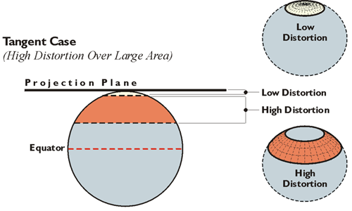
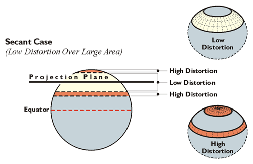
Decreasing distortion is a constant and elusive goal in map projection. It can be done in several ways. Most involve reducing the distance between the map projection surface and the ellipsoidal surface. One way this is done is to move the mapping surface from tangency with the ellipsoid and make it actually cut through it. This strategy produces what is known as a secant projection. A secant projection is one way to shrink the distance between the map projection surface and the ellipsoid. Thereby, the area where distortion is in an acceptable range on the map can be effectively increased. The illustrations here are intended to show how the tangent case distorts a larger area than does the secant case. The tangent on the top shows a flat projection plane touching the Earth at one point. This is the approach used in polar protections (North Pole, South Pole). The area in orange has high distortion. The low distortion, the area in the light beige, is much smaller. However, if the projection plane cuts the Earth rather than just touching it at one point, there's a larger area of relatively low distortion. The less the distance between the plane and the Earth, the less the distortion. (The areas on the Earth closest to the plane have less distortion than the areas farther away from the plane.) The secant case has lower distortion over a larger area than does the tangent case. This is why State Plane coordinate systems in the United States use secant projections. In the case of Lambert projection, there are two parallels of latitude where the mapping plane cuts the Earth. In the case of Transverse Mercator, there are two approximately north-south lines that are not meridian of longitude. In both cases, these are lines of exact scale.
Both cones and cylinders have an advantage over a flat map projection plane. They are curved in one direction and can be designed to follow the curvature of the area to be mapped in that direction. Also, if a large portion of the ellipsoid is to be mapped, several cones or several cylinders may be used together in the same system to further limit distortion. In that case, each cone or cylinder defines a zone in a larger coverage. This is the approach used in State Plane Coordinate systems. Generally, one cone or one cylinder is not sufficient to cover an entire state (though there are exceptions). Usually a collection of cones or cylinders, one for each zone, is used. That's the approach that was used in the original design of most State Plane coordinate systems in this country.
Secant Projections
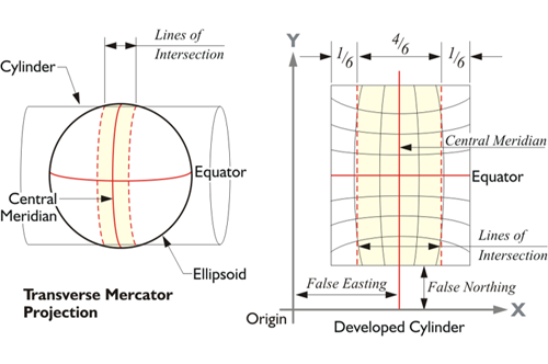
As mentioned, when a conic or a cylindrical map projection surface is made secant, it intersects the ellipsoid, and the map is brought close to its surface. For example, the conic and cylindrical projections shown in the illustration cut through the ellipsoid. The map is projected both inward and outward onto it and there is no distortion on the two lines of exact scale, standard lines. They are created along the small circles where the cone and the cylinder intersect the ellipsoid. They are called small circles because they do not describe a plane that goes through the center of the Earth, as do the previously mentioned great circles. Between the standard lines, the map is under the ellipsoid, and outside of the standard lines, the map is above it. That means that between the standard lines, a distance from one point to another is actually longer on the ellipsoid than it is shown on the map, and outside the standard lines, a distance on the ellipsoid is shorter than it is on the map. Any length that is measured along a standard line is the same on the ellipsoid and on the map, which is why another name for standard parallels is lines of exact scale. They are called standard parallels in the case of a Lambert projection that is illustrated at the top here. The lower picture is Transverse Mercator projection and the lines of exact scale neither meridians of longitude nor parallels of latitude, but are rather complex curves,
Conformal
Ultimately, the goal is very straightforward relating each position on one surface, the reference ellipsoid, to a corresponding position on another surface as faithfully as possible and then flattening that second surface to accommodate Cartesian coordinates. In fact, the whole procedure is in the service of moving from geographic to Cartesian coordinates and back again. These days, the complexities of the mathematics are handled with computers. Of course, that was not always the case. Map projections in which shape is preserved are known as conformal or orthomorphic. Orthomorphic means right shape. In a conformal projection, the angles between intersecting lines and curves retain their original form on the map. In other words, between short lines, meaning lines under about 10 miles, a 45º angle on the ellipsoid is a 45º angle on the map. It also means that the scale is the same in all directions from a point; in fact, it is this characteristic that preserves the angles. These aspects were certainly a boon for all State Plane Coordinate users. On long lines, angles on the ellipsoid are not exactly the same on the map projection. Nevertheless, the change is small and systematic. Actually, all three of the projections that were used in the designs of the original State Plane Coordinate Systems were conformal. Each system was originally based on the North American Datum 1927, NAD27. Along with the Oblique Mercator projection, which was used on the panhandle of Alaska, the two primary projections were the Lambert Conic Conformal Projection and the Transverse Mercator projection. Today, they're in North American Datum of 1983, NAD83 2011 (2010.0).
Projection Design
In 1932, two engineers in North Carolina’s highway department, O.B. Bester and George F. Syme, appealed to the then Coast & Geodetic Survey (C&GS, now NGS) for help. They had found that the stretching and compression inevitable in the representation of the curved earth on a plane was so severe over long route surveys that they could not check into the C&GS geodetic control stations across a state within reasonable limits. The engineers suggested that a plane coordinate grid system be developed that was mathematically related to the reference ellipsoid, but could be utilized using plane trigonometry rather than laborious geodetic calculations because in those days such calculations required sharp pencils, logarithmic tables and lots of midnight oil. Dr. Oscar Adams of the Division of Geodesy, assisted by Charles Claire, designed the first State Plane Coordinate System to mediate the problem. It was based on a map projection called the Lambert Conformal Conic Projection. Adams realized that it was possible to use this map projection and allow one of the four elements of area, shape, scale, or direction to remain virtually unchanged from its actual value on the earth, but not all four. On a perfect map projection, all distances, directions, and areas could be conserved. They would be the same on the ellipsoid and on the map. Unfortunately, it is not possible to satisfy all of these specifications simultaneously, at least not completely. There are inevitable choices. It must be decided which characteristic will be shown the most correctly, but it will be done at the expense of the others. And there is no universal best decision. Still, a solution that gives the most satisfactory results for a particular mapping problem is always available.
On the Lambert Conformal Conic Projection, parallels of latitude are arcs of concentric circles, and meridians of longitude are equally spaced straight radial lines, and the meridians and parallels intersect at right angles. The axis of the cone is imagined to be a prolongation of the polar axis. The parallels are not equally spaced because the scale varies as you move north and south along a meridian of longitude. Adams decided to use this map projection in which shape is preserved based on a developable cone. The Transverse Mercator projection is based on a cylindrical mapping surface much like that illustrated here. However, the axis of the cylinder is rotated so that it is perpendicular with the polar axis of the ellipsoid. Unlike the Lambert Conic projection, the Transverse Mercator represents meridians of longitude as curves rather than straight lines on the developed grid. The Transverse Mercator projection is not the same thing as the Universal Transverse Mercator system (UTM). UTM was originally a military system that covers the entire earth and differs significantly from the Transverse Mercator system used in State Plane Coordinates.
In using these projections as the foundation of the State Plane Coordinate systems, Adams wanted to have the advantage of conformality and also cover each state with as few zones as possible. A zone in this context is a belt across the state that has one Cartesian coordinate grid with one origin and is projected onto one mapping surface. One strategy that played a significant role in achieving that end was Adams’s use of secant projections in both the Lambert and Transverse Mercator systems. Using a single secant cone in the Lambert projection and limiting the extent of a zone, or belt, across a state to about 158 miles, approximately 254 km, Dr. Adams limited the distortion of the length of lines. Not only were angles preserved in the final product, but also there were no radical differences between the length of a measured line on the Earth’s surface and the length of the same line on the map projection. In other words, the scale of the distortion was small.
He placed 4/6th of the map projection plane between the standard lines, 1/6th outside at each extremity. The distortion was held to 1 part in 10,000. A maximum distortion in the lengths of lines of 1 part in 10,000 means that the difference between the length of a 2-mile line on the ellipsoid and its representation on the map would be about 1 foot. State Plane Coordinates were created to be the basis of a method that approximates geodetic accuracy more closely than the then commonly used methods of small-scale plane surveying. Today, surveying methods can easily achieve accuracies far beyond those prevalent in those days, but the State Plane Coordinate systems were designed in a time of generally lower accuracy and efficiency in surveying measurement.
The original State Plane Coordinate System (SPCS) was so successful in North Carolina, similar systems were devised for all the states in the Union within a year or so. The system was successful because, among other things, it overcame some of the limitations of mapping on a horizontal plane while avoiding the imposition of strict geodetic methods and calculations. It managed to keep the distortion of the scale ratio under 1 part in 10,000 and preserved conformality. It did not disturb the familiar system of ordered pairs of Cartesian coordinates, and it covered each state with as few zones as possible whose boundaries were constructed to follow county lines. County lines were generally used, so that those relying on State Plane Coordinates could work in one zone throughout a jurisdiction.
State Plane Coordinate Zones 1983, False Eastings and Scale

In several instances, the boundaries of State Plane Coordinate Zones today, SPCS83, the State Plane Coordinate System based on NAD83 2011 (2010.0) and its reference ellipsoid GRS80, differ from the original zone boundaries. The foundation of the original State Plane Coordinate System, SPCS27 was NAD27 and its reference ellipsoid Clarke 1866. As mentioned earlier, NAD27 geographical coordinates, latitudes and longitudes, differ significantly from those in NAD83 2011 (2010.0). In fact, conversion from geographic coordinates, latitude and longitude, to grid coordinates, y and x, and back is one of the three fundamental conversions in the State Plane Coordinate system. It is important because the whole objective of the SPCS is to allow the user to work in plane coordinates, but still have the option of expressing any of the points under consideration in either latitude and longitude or State Plane Coordinates without significant loss of accuracy. Therefore, when geodetic control was migrated from NAD27 to NAD83 2011 (2010.0), the State Plane Coordinate System had to go along. When the migration was undertaken in the 1970s, it presented an opportunity for an overhaul of the system. Many options were considered, but in the end, just a few changes were made. One of the reasons for the conservative approach was the fact that 37 states had passed legislation supporting the use of State Plane Coordinates. Nevertheless, some zones got new numbers, and some of the zones changed. The zones are numbered in the SPCS83 system known as FIPS. FIPS stands for Federal Information Processing Standard, and each SPCS83 zone has been given a FIPS number. These days, the zones are often known as FIPS zones. SPCS27 zones did not have these FIPS numbers. As mentioned earlier, the original goal was to keep each zone small enough to ensure that the scale distortion was 1 part in 10,000 or less, but when the SPCS83 was designed, that scale was not maintained in some states. In five states, some SPCS27 zones were eliminated altogether and the areas they had covered were consolidated into one zone or added to adjoining zones. In three of those states, the result was one single large zone. Those states are South Carolina, Montana, and Nebraska. In SPCS27, South Carolina and Nebraska had two zones; in SPCS83, they have just one, FIPS zone 3900 and FIPS zone 2600, respectively. Montana previously had three zones. It has one, FIPS zone 2500. Therefore, because the area covered by these single zones has become so large, they are not limited by the 1 part in 10,000 standard. California eliminated zone 7 and added that area to FIPS zone 0405, formerly zone 5. Two zones previously covered Puerto Rico and the Virgin Islands. They have one. It is FIPS zone 5200. In Michigan, three Transverse Mercator zones were entirely eliminated.
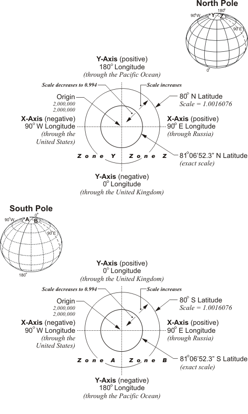
In both the Transverse Mercator and the Lambert Conic projection, the positions of the axes are similar in all SPCS zones. As you can see in the illustration, each zone has a central meridian. These central meridians are true meridians of longitude near the geometric center of the zone. Please note that the central meridian is not the y-axis. If it were the y-axis negative coordinates would result. To avoid them, the actual y-axis is moved far to the west of the zone itself. In the old SPCS27 arrangement, the y-axis was 2,000,000 feet west from the central meridian in the Lambert Conic projection and 500,000 feet in the Transverse Mercator projection. In the SPCS83 design, those constants have been changed. The most common values are 600,000 meters for the Lambert Conic and 200,000 meters for the Transverse Mercator. However, there is a good deal of variation in these numbers from state to state and zone to zone. In all cases, however, the y-axis is still far to the west of the zone and there are no negative State Plane Coordinates. No negative coordinates, because the x-axis, also known as the baseline, is far to the south of the zone. Where the x-axis and y-axis intersect is the origin of the zone, and that is always south and west of the zone itself. This configuration of the axes ensures that all State Plane Coordinates occur in the first quadrant and are, therefore, always positive.
It is important to note that the fundamental unit for SPCS27 was the U.S. survey foot, but "the U.S. survey foot will be phased out as part of the modernization of the National Spatial Reference System (NSRS). From this point forward, the international foot will be simply called the foot." https://www.nist.gov/pml/us-surveyfoot. The fundamental unit for SPCS83, it is the meter.
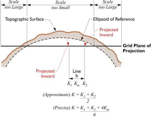
This brings us to the scale factor, also known as the K factor and the projection factor. It was this factor that the original design of the State Plane Coordinate system sought to limit to 1 part in 10,000. As implied by that effort, scale factors are ratios that can be used as multipliers to convert ellipsoidal lengths, also known as geodetic distances, to lengths on the map projection surface, also known as grid distances, and vice versa. Please notice that the geodetic distance is the distance on the ellipsoid of reference, not the distance measured on the surface of the earth. So, the geodetic length of a line, on the ellipsoid, multiplied by the appropriate scale factor will give you the grid length of that line on the state plane (the map). And the grid length multiplied by the inverse of that same scale factor would bring you back to the geodetic length again. There's another factor that will get you from topographic surface of the earth —where the measurement was made— down to the ellipsoid. However, at the moment we're talking about the scale factor. Here in this image, you see a state plane, and a horizontal line is indicated between the bases of the red arrows. Please notice that between the standard lines, the scale is too small on the state plane. And outside the standard lines, the scale is too large on the state plane. So, the line between the bases of those two red arrows on the ellipsoid of reference will be projected inward from the ellipsoid to the state plane. As it's projected inward —the line shortens. That means that between the intersection of standard lines, the grid (state plane) is under the ellipsoid. In that area, a distance from one point to another is longer on the ellipsoid than on the state plane. This means that right in the middle of the State Plane coordinate systems zone, the scale is at its minimum. In the middle, a typical minimum State Plane coordinate scale factor is not less than 0.9999. Outside of the standard lines, the grid (state plane) is above the ellipsoid where the distance from one point to another is shorter on the ellipsoid than it is on the state plane. There, at the edge of the zone, a maximum typical State Plane coordinate system scale factor is generally not more than 1.0001.
The projection used most on states that are longest from east to west is the Lambert Conic. In this projection, the scale factor for east-west lines is constant. In other words, the scale factor is the same all along the line. One way to think about this is to recall that the distance between the ellipsoid and the map projection surface does not change east to west in that projection. On the other hand, along a north-south line, the scale factor is constantly changing on the Lambert Conic. And it is no surprise then to see that the distance between the ellipsoid and the map projection surface is always changing along the north to south line in that projection. But looking at the Transverse Mercator projection, the projection used most on states longest north to south, the situation is exactly reversed. In that case, the scale factor is the same all along a north-south line, and changes constantly along an east-west line.
Both the Transverse Mercator and the Lambert Conic used a secant projection surface and originally restricted the width to 158 miles. These were two strategies used to limit scale factors when the State Plane Coordinate systems were designed. Where that was not optimum, the width was sometimes made smaller, which means the distortion was lessened. As the belt of the ellipsoid projected onto the map narrows, the distortion gets smaller. For example, Connecticut is less than 80 miles wide north to south. It has only one zone. Along its northern and southern boundaries, outside of the standard parallels, the scale factor is 1 part in 40,000, a fourfold improvement over 1 part in 10,000. And in the middle of the state, the scale factor is 1 part in 79,000, nearly an eightfold increase. On the other hand, the scale factor was allowed to get a little bit smaller than 1 part in 10,000 in Texas. By doing that, the state was covered completely with five zones. And among the guiding principles in 1933 was covering the states with as few zones as possible and having zone boundaries follow county lines. Still it requires ten zones and all three projections to cover Alaska.
When SPCS 27 was current, scale factors were interpolated from tables published for each state. In the tables for states in which the Lambert Conic projection was used, scale factors change north–south with the changes in latitude. In the tables for states in which the Transverse Mercator projection was used, scale factors change east-west with the changes in x-coordinate. Today, scale factors are not interpolated from tables for SPCS83. For both the Transverse Mercator and the Lambert Conic projections, they are calculated directly from equations. There are also several software applications that can be used to automatically calculate scale factors for particular stations. They can be used to convert latitudes and longitudes to State Plane Coordinates. Given the latitude and longitude of the stations under consideration, part of the available output from these programs is typically the scale factors for those stations. To illustrate the use of these factors, consider a line with a length on the ellipsoid of 130,210.44 feet, a bit over 24 miles. That would be its geodetic distance. Suppose that the scale factor for that line was 0.9999536, then the grid distance along the line would be:
Geodetic Distance * Scale Factor = Grid Distance
130,210.44 ft. * 0.999953617 = 130,204.40 ft.
The difference between the longer geodetic distance and the shorter grid distance here is a little more than 6 feet. That is actually better than 1 part in 20,000; please recall that the 1 part in 10,000 ratio was originally considered the maximum. Distortion lessens, and the scale factor approaches 1 as a line nears a standard parallel. Please also recall that on the Lambert projection, an east–west line, that is a line that follows a parallel of latitude, has the same scale factor at both ends and throughout. However, a line that bears in any other direction will have a different scale factor at each end. A north–south line will have a great difference in the scale factor at its north end compared with the scale factor of its south end.
Where K is the scale factor for a line, K1 is the scale factor at one end of the line and K2 is the scale factor at the other end of the line. Scale factor varies with the latitude in the Lambert projection. For example, suppose the point at the north end of the 24-mile line is called Stormy and has a geographic coordinate of:
37º46’00.7225”
103º46’35.3195”
and at the south end the point is known as Seven with a geographic coordinate of:
37º30’43.5867”
104º05’26.5420”
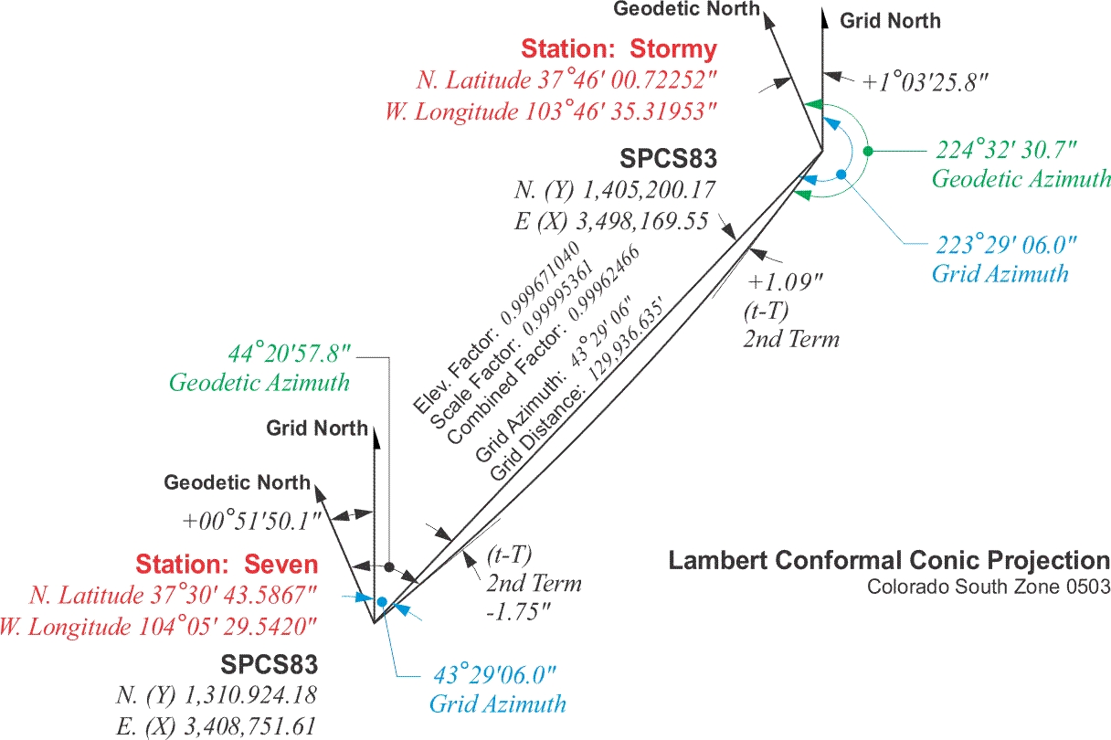
The scale factor for point Seven is 0.99996113 and the scale factor for point Stormy is 0.99994609. It happens that point Seven is further south and closer to the standard parallel than is point Stormy, and it therefore follows that the scale factor at Seven is closer to 1. It would be exactly 1 if it were on the standard parallel, which is why the standard parallels are called lines of exact scale. The typical scale factor for the line is the average of the scale factors at the two end points:
Deriving the scale factor at each end and averaging them is the usual method for calculating the scale factor of a line. The average of the two is sometimes called Km.
However, it can also be done by the precise method K = K1 + K2 + 4Km/6
Elevation Factor
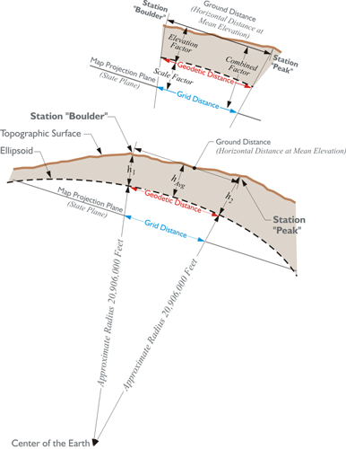
But, that is not the whole story when it comes to reducing distance to the State Plane Coordinate grid. Measurement of lines must always be done on the topographic surface of the Earth, and not on the ellipsoid. Therefore, the first step in deriving a grid distance must be moving a measured line from the Earth to the ellipsoid. The scale factor moves us from the ellipsoid to the state plane (aka grid). However, as mentioned here, the measurements are not made on the ellipsoid. They are made on the surface of the Earth. If we're going to measure the line from one point to another — from station Boulder to station Peak as shown in the illustration— that distance would be measured on the surface of the Earth. To move from the surface of the Earth down to the ellipsoid, we need to have what's known as an elevation factor. Typically, the elevation factor for a line is the average of the elevation factors at each end of the line. For example, the average of the elevation factor at station Boulder (h1), and the elevation factor at station Peak (h2) is the elevation factor for the line (hAvg). That would give the elevation factor for the line Boulder-Peak. Once the elevation factor is available, it is multiplied with the scale factor. The result is known as the combined factor. The combined factor will move the line from the topographic surface of the Earth to the state plane (aka grid).
In the illustration, you may have noticed the approximate radius of the Earth, 20,906,000 feet. It is shown from the center of mass of the Earth up to the ellipsoid. It is an approximation used in creating this elevation factor.
In other words, converting a distance measured on the topographic surface to a geodetic distance on the reference ellipsoid is done with another ratio that is also used as a multiplier. Originally, this factor had a rather unfortunate name. It used to be known as the sea level factor in SPCS27. It was given that name because as you may recall that when NAD27 was established using the Clarke 1866 reference ellipsoid, the distance between the ellipsoid and the geoid was declared to be zero at Meades Ranch in Kansas. That meant that in the middle of the country the sea level surface, the geoid, and the ellipsoid were coincident by definition. And since the Clarke 1866 ellipsoid fit the United States quite well, the separation between the two surfaces, the ellipsoid and geoid, only grew to about 12 meters anywhere in the country. With such a small distance between them, many practitioners at the time took the point of view that, for all practical purposes, the ellipsoid and the geoid were in the same place. And that place was called sea level. Hence, reducing a distance measure on the surface of the Earth to the ellipsoid was said to be reducing it to sea level.
Today, that idea and that name for the factor are misleading because, of course, the GRS80 ellipsoid on which NAD83 is based is certainly not the same as Mean Sea Level. The separation between the geoid and ellipsoid can grow as large as 53 meters. And technology by which lines are measured has improved dramatically. Therefore, in SPCS83, the factor for reducing a measured distance to the ellipsoid is known as the ellipsoid factor. In any case, both the old and the new name can be covered under the name the elevation factor. Regardless of the name applied to the factor, it is a ratio. The ratio is the relationship between an approximation of the Earth’s radius and that same approximation with the mean ellipsoidal height of the measured line added to it. For example, consider station Boulder and station Peak illustrated in the figure above.
Boulder
- N39º59’29.1299”
- W105º15’39.6758”
Peak
- N40º01’19.1582”
- W105º30’55.1283”
The distance between these two stations is 72,126.21 feet. This distance is sometimes called the ground distance, or the horizontal distance at mean elevation. In other words, it is not the slope distance but rather the distance between them corrected to an averaged horizontal plane, as is common practice. For practical purposes, then, this is the distance between the two stations on the topographic surface of the Earth. On the way to finding the grid distance Boulder to Peak, there is the interim step, calculating the geodetic distance between them, that is the distance on the ellipsoid. We need the elevation factor, and here is how it is determined.
The ellipsoidal height of Boulder, h1, is 5,437 feet. The ellipsoidal height of Peak, h2, is 9,099 feet. The approximate radius of the Earth, traditionally used in this work, is 20,906,000 feet. The elevation factor is calculated:
This factor then is the ratio used to move the ground distance down to the ellipsoid, down to the geodetic distance.
It is possible to refine the calculation of the elevation factor by using an average of the actual radial distances from the center of the ellipsoid to the end points of the line, rather than the approximate 20,906,000 feet. In the area of stations Boulder and Peak, the average ellipsoidal radius is actually a bit longer, but it is worth noting that within the continental United States such variation will not cause a calculated geodetic distance to differ significantly.
Grid and Geodetic Azimuths

You will find that every zone in a State Plane coordinate system has a central meridian. In Colorado, the central meridian is 105 degrees, 30 minutes West Longitude, as shown here, on the left you have station D266 and on the right, station Fink. Notice that, in both cases, that grid north is exactly parallel with the central meridian. This is the convention for any plane coordinate system, so that north is always up, and always the same direction. All the norths are parallel in the plane systems; this is, of course, unrealistic. Meridians converge on the surface of the Earth. Therefore, there is a value, shown here in blue, called convergence. Convergence is the difference between geodetic north and grid north. You see over here on the right at station Fink, the convergence is plus 17.2 arcseconds. All the convergence angles east of the Central Meridian are positive. On the left, at station D266, the convergence is minus 40.0 arcseconds. All the convergence angles west of the Central Meridian are negative.
Please note that the sum of the grid azimuths (in red) at station Fink and station D266 is 360 degrees. This is a direct result of the grid north lines being parallel with each other. However, the sum of the geodetic azimuths (in green) at station Fink and station D266 is not 360 degrees. This is a direct result of the geodetic north lines converging. On the Earth they are not parallel with each other. The bottom line is this. On the State Plane coordinate grid, north is always parallel with the central meridian, but at the points on the Earth, north is along the meridian that passes through them. They are certainly not parallel with one another and certainly not parallel with the central meridian.
Universal Transverse Mercator
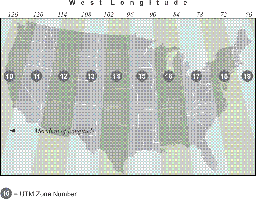
A plane coordinate system that is convenient for GIS work over large areas is the Universal Transverse Mercator (UTM) system. UTM with the Universal Polar Stereographic system covers the world in one consistent system. It is four times less precise than typical State Plane Coordinate systems, with a scale factor that reaches 0.9996. A Universal Transverse Mercator zone embraces a much larger portion of the earth than does a state plane coordinate zone. When you get a larger bite, a larger portion of the earth, the scale factor is less attractive. Yet, the ease of using UTM and its worldwide coverage makes it very attractive for work that would otherwise have to cross many different SPCS zones. For example, nearly all National Geospatial-Intelligence Agency (NGA) topographic maps, U.S. Geological Survey (USGS) quad sheets, and many aeronautical charts show the UTM grid lines. It is often said that UTM is a military system created by the U.S. Army; but several nations, and the North Atlantic Treaty Organization (NATO), played roles in its creation after World War II. At that time, the goal was to design a consistent coordinate system that could promote cooperation between the military organizations of several nations. Before the introduction of UTM, allies found that their differing systems hindered the synchronization of military operations. Conferences were held on the subject from 1945 to 1951, with representatives from Belgium, Portugal, France, and Britain, and the outlines of the present UTM system were developed. By 1951, the U.S. Army introduced a system that was very similar to that currently used. The UTM projection divides the world into 60 zones that begin at longitude 180º, the International Date Line. Zone 1 is from 180° to the 174° W longitude. The conterminous United States is within UTM zones 10 to 19. Here is a convenient way to find the zone number for a particular longitude. Consider west longitude negative and east longitude positive, add 180° and divide by 6. Any answer greater than an integer is rounded to the next highest integer, and you have the zone. For example, Denver, Colorado is near 105° W. Longitude, –105°.
–105° + 180° = 75°
75 °/ 6 = 12.50<
Round up to 13
Therefore, Denver, Colorado, is in UTM Zone 13.
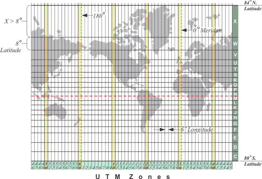
All UTM zones have a width of 6° of longitude. From north to south, the zones extend from 84° N latitude to 80° S latitude. Originally the northern limit was at 80° N latitude and the southern 80° S latitude. On the south, the latitude is a small circle that conveniently traverses the ocean well south of Africa, Australia, and South America. However, 80° N latitude was found to exclude parts of Russia and Greenland and was extended to 84° N latitude. You will notice letters of the alphabet along the right edge of the illustration. There are a few letters missing. You see C,D,E, F, G,H —but there is no I, because it's too close to the number 1 and could be confused— J,K, L, M, N —but there is no O, it could be confused for the number zero— P,Q, R, S,T U, V, W, X, there is no Y, — and finally there is Z. I point this out because there are GPS/GNSS systems that use these letter designations along with the number of the UTM zone to identify a particular quadrangle. For example, C21 would be the square that you see just immediately above 21 in the Southern Hemisphere. This is a useful method of referring to a particular quadrangle in a particular UTM zone. The designations are also used by the military.
Unlike any of the systems previously discussed, every coordinate in a UTM zone occurs twice, once in the Northern Hemisphere and once in the Southern Hemisphere. This is a consequence of the fact that there are two origins in each UTM zone. The origin for the portion of the zone north of the equator is moved 500 km west of the intersection of the zone’s central meridian and the equator. This arrangement ensures that all of the coordinates for that zone in the Northern Hemisphere will be positive. The origin for the coordinates in the Southern Hemisphere for the same zone is 500 km west of the central meridian, as well. But in the Southern Hemisphere, the origin is not on the equator, it is 10,000 km south of it, close to the South Pole. This orientation of the origin guarantees that all of the coordinates in the Southern Hemisphere are in the first quadrant and are positive. In other words, the intersection of each zone’s central meridian with the equator defines its origin of coordinates. In the southern hemisphere, each origin is given the coordinates:
easting = X0 = 500, 000 meters, and northing = Y0 = 10,000,000 meters
In the northern hemisphere, the values are:
easting = X0 = 500, 000 meters, and northing = Y0 = 0 meters, at the origin
The UTM zones nearly cover the earth, except the Polar Regions, which are covered by two azimuthal polar zones called the Universal Polar Stereographic (UPS) projection.
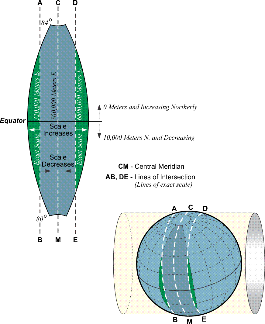
The foundation of the 60 UTM zones is a secant Transverse Mercator projection, very similar to those used in some State Plane Coordinate systems. The central meridian of the zones is exactly in the middle. For example, in Zone 1, from 180° W to the 174° W longitude, the central meridian is 177° W longitude, so each zone extends 3 degrees east and west from its central meridian. The UTM secant projection gives approximately 180 kilometers between the lines of exact scale where the cylinder intersects the ellipsoid. The scale factor grows from 0.9996 along the central meridian of a UTM zone to 1.00000 at 180 km to the east and west. Please recall that SPCS zones are usually more limited in width, ~158 miles, and, therefore, have a smaller range of scale factors than do the UTM zones. In State Plane coordinates, the scale factor is usually no more than 1 part in 10,000. In UTM coordinates, it can be as large as 1 part in 2500. The reference ellipsoids for UTM coordinates vary.
Heights
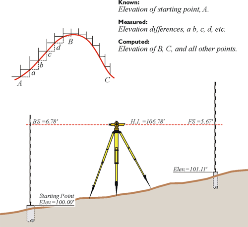
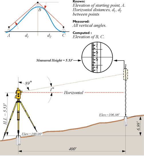
A point on the earth’s surface is not completely defined by its latitude and longitude. In such a context, there is, of course, a third element, that of height. Surveyors have traditionally referred to this component of a position as its elevation. One classical method of determining elevations is spirit leveling. A level, correctly oriented at a point on the surface of the earth, defines a line parallel to the geoid at that point. Therefore, the elevations determined by level circuits are orthometric; that is, they are defined by their vertical distance above the geoid as it would be measured along a plumb line. However, orthometric elevations are not directly available from the geocentric position vectors derived from GPS/GNSS measurements. In a normal course of things, a coordinate —YX, or northing easting, or latitude and longitude— is not fully a definition of a position. We've discussed also Earth-Centered, Earth-Fixed XYZ coordinates, but it is typical for a horizontal coordinate to be given a height, or elevation. This third element, was most often originally determined by spirit leveling or, in some cases, by a technique known as trigonometric leveling. Despite the surveying method that was used in the past, it was based on optical instruments oriented to gravity, therefore oriented to the geoid. Therefore, the heights were based upon gravity. There is a long legacy of benchmarks, recorded heights, and archives that are based upon this sort of methodology of determining heights. And so, this is what it follows that these values are generally what we think of as elevations —we think of orthometric heights based upon gravity.
Ellipsoidal Heights
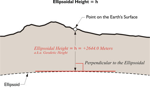
As mentioned before, modern geodetic datums rely on the surfaces of geocentric ellipsoids to approximate the surface of the Earth. But the actual surface of the Earth does not coincide with these nice smooth surfaces, even though that is where the points represented by the coordinate pairs lay. Abstract points may be on the ellipsoid, but the physical features those coordinates intend to represent are on the Earth. Though the intention is for the Earth and the ellipsoid to have the same center, the surfaces of the two figures are certainly not in the same place. There is a distance between them. The distance represented by a coordinate pair on the reference ellipsoid to the point on the surface of the Earth can be measured along a line perpendicular to the ellipsoid - which differs from the direction of gravity. This distance is known by more than one name. It is called the ellipsoidal height, and it is also called the geodetic height and is usually symbolized by h. In the illustration, you see an ellipsoidal height of +2,644 meters. The concept is straightforward. A reference ellipsoid may be above or below the surface of the Earth at a particular place. If the ellipsoid’s surface is below the surface of the Earth at the point, the ellipsoidal height has a positive sign; if the ellipsoid’s surface is above the surface of the Earth at the point, the ellipsoidal height has a negative sign.
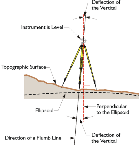
It is quite impossible to actually set up an instrument on the ellipsoid. That makes it tough to measure ellipsoidal height using surveying instruments. In other words, ellipsoidal height is not what most people think of as an elevation. Said another way, an ellipsoidal height is not measured in the direction of gravity. It is not measured in the conventional sense of down or up. In the illustration, there is an instrument level on the topographic surface of the Earth. The direction of gravity does not coincide with the perpendicular to the ellipsoid.
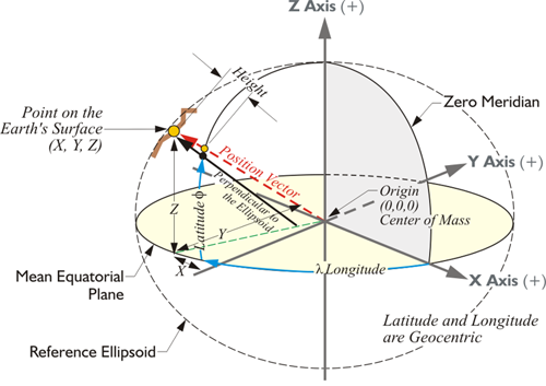
Nevertheless, the ellipsoidal height of a point is readily determined using a GPS/GNSS receiver. GPS/GNSS can be used to discover the distance from the geocenter of the Earth to any point on the Earth, or above it for that matter. In other words, it has the capability of determining three-dimensional coordinates of a point in a short time. It can provide latitude and longitude, and if the system has the parameters of the reference ellipsoid in its software, it can calculate the ellipsoidal height. The relationship between points can be further expressed in the ECEF coordinates, X, Y, and Z, or in a Local Geodetic Horizon System (LHGS) of north, east, and up. Actually, in a manner of speaking, ellipsoidal heights are new, at least in common usage, since they could not be easily determined until GPS/GNSS became a practical tool in the 1980s.
You may wonder why in the world spend any time at all on this bizarre idea of an ellipsoid height. Since you can't measure it directly, you can't set up on the ellipsoid, what's the point? Well, here's the point. As you see in this image, the ellipsoid height, not the orthometric height, is what is determined directly from a GPS/GNSS measurement. The GPS/GNSS satellites orbit around the center of mass of the Earth. They have no concept of where the surface of the Earth is. Your receiver, which is on the surface of the Earth, of course, could just as well be in outer space as far as the GPS/GNSS coordinate or Earth-Centered-Earth-Fixed XYZ is concerned. Starting from the 3D Cartesian coordinate and given a particular ellipsoid on which to work, it is possible for the computer in your GPS/GNSS receiver to calculate a latitude and longitude. It will base that latitude and longitude on the ellipsoidal parameters in its microcomputer. It follows that the height that is determined up to the station that you're interested in will also be based upon the ellipsoid.
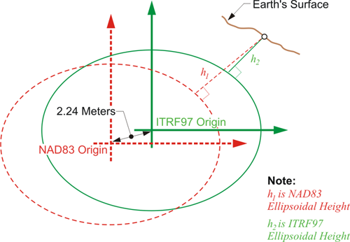
However, ellipsoidal heights are not all the same, because reference ellipsoids, or sometimes just their origins, can differ. For example, an ellipsoidal height expressed in ITRF might be based on an ellipsoid with exactly the same shape as the NAD83 ellipsoid, GRS80. Nevertheless, the heights would be different because the origin has a different relationship with the Earth’s surface. It's worthwhile to note that ellipsoidal heights vary as the ellipsoid changes. As the reference frame (datum) changes, the ellipsoid height changes. And that's what this image here is intended to represent. There is an approximately 2.24 meter separation between the origin of NAD83, the GRS80 ellipsoid, the ITRF ellipsoid. Therefore, the heights —the small h, the ellipsoid height— derived from each of these would be different.
The Geoid
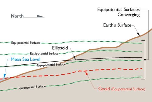
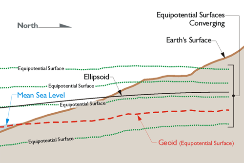
Any object in the earth’s gravitational field has potential energy derived from being pulled toward the Earth. Quantifying this potential energy is one way to talk about height, because the amount of potential energy an object derives from the force of gravity is related to its height. There are an infinite number of points where the potential of gravity is always the same. They are known as equipotential surfaces. Mean Sea Level itself is not an equipotential surface at all, of course. Forces other than gravity affect it, forces such as temperature, salinity, currents, wind, and so forth. The geoid, on the other hand, is defined by gravity alone. The geoid is the particular equipotential surface arranged to fit Mean Sea Level as well as possible, in at least squares sense. The geoid and the ellipsoid are not the same. Remember that the legacy heights determined by optical instruments in the past were always relative to the geoid, because, of course, the instruments were oriented to gravity. However, GPS/GNSS heights are related directly at least to the ellipsoid —two different surfaces.
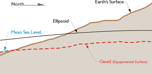
So, while there is a relationship between Mean Sea Level and the geoid, they are not the same. They could be the same if the oceans of the world could be utterly still, completely free of currents, tides, friction, variations in temperature, and all other physical forces, except gravity. However, these unavoidable forces actually cause Mean Sea Level to deviate up to 1, even 2, meters from the geoid.
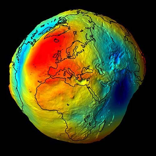
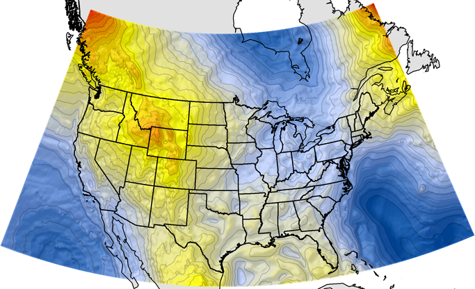
The geoid is completely is not smooth and continuous. It is lumpy, because gravity is not consistent across the surface of the earth. At every point, gravity has a magnitude and a direction, but these vectors do not all have the same direction or magnitude. Some parts of the earth are denser than others. Where the earth is denser, there is more gravity, and the fact that the earth is not a sphere also affects gravity. The geoid undulates with the uneven distribution of the mass of the earth and has all the irregularity that the attendant variation in gravity implies. In fact, the separation between the lumpy surface of the geoid and the smooth GRS80 ellipsoid worldwide varies from about +85 meters west of Ireland to about -106 meters, the latter in the area south of India near Ceylon.
In the conterminous United States, sometimes-abbreviated CONUS, the distances between the geoid and the GRS80 ellipsoid, known as geoid heights, are less. They vary from about –8 meters to about –53 meters.
Height Conversion
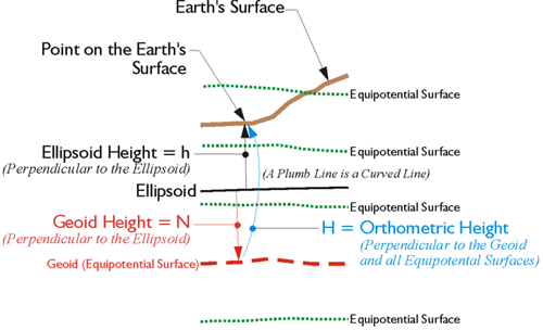
A geoidal height is the distance measured along a line perpendicular to the ellipsoid of reference to the geoid. Also, as you can see in the illustration, these geoid heights are negative. They are usually symbolized, N. If the geoid is above the ellipsoid, N is positive; if the geoid is below the ellipsoid, N is negative. It is negative here because the geoid is underneath the ellipsoid throughout the conterminous United States. In Alaska, it is the other way around; the ellipsoid is underneath the geoid and N is positive.
Please recall that an ellipsoid height is symbolized, h. The ellipsoid height is also measured along a line perpendicular to the ellipsoid of reference, but to a point on the surface of the Earth.
However, an orthometric height, symbolized, H, is measured along a plumb line from the geoid to a point on the surface of the Earth. By using the formula,
H = h – N
one can convert an ellipsoidal height, h, derived say from a GPS/GNSS observation, into an orthometric height, H, by knowing the extent of geoid-ellipsoid separation, also known as the geoidal height, N, at that point. The ellipsoid height of a particular point is actually smaller than the orthometric height throughout the conterminous United States.
The formula H = h – N does not account for the fact that the plumb line along which an orthometric height is measured is curved, as you see in the figure above. Curved, because it is perpendicular with each and every equipotential surface through which it passes. The equipotential surfaces are not parallel with each other. They converge toward the pole because the Earth is oblate therefore, the plumb line must curve to maintain perpendicularity with them all. This deviation of a plumb line from the perpendicular to the ellipsoid reaches about 1 minute of arc in only the most extreme cases. Therefore, any height difference that is caused by the curvature is negligible. It would take a height of over 6 miles for the curvature to amount to even 1 mm of difference in height.
Geoidal Models
Major improvements have been made over the past quarter-century or so in mapping the geoid on both national and global scales. And because there are large complex variations in the geoid related to both the density and relief of the earth, geoid models and interpolation software have been developed to support the conversion of GPS elevations to orthometric elevations. For example, in early 1991, NGS presented a program known as GEOID90. This program allowed a user to find N, the geoidal height, in meters for any NAD83 latitude and longitude in the United States.
The GEOID90 model was computed at the end of 1990, using over a million gravity observations. It was followed by the GEOID93 model. It was computed at the beginning of 1993, using more than 5 times the number of gravity values used to create GEOID90. Both provided a grid of geoid height values in 3 minutes of latitude by 3 minutes of longitude grid with an accuracy of about 10 cm. Next, the GEOID96 model resulted in a gravimetric geoid height grid in a 2 minutes of latitude by 2 minutes of longitude grid.
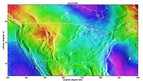
GEOID99 covered the conterminous United States, and it includes U.S. Virgin Islands, Puerto Rico, Hawaii, and Alaska. The grid is 1 degree of latitude by 1 degree of longitude, and it is the first to combine gravity values with GPS ellipsoid heights on previously leveled benchmarks. According to NGS, “When comparing the GEOID99 model with GPS ellipsoid heights in the NAD 83 reference frame and leveling in the NAVD 88 datum, it is seen that GEOID99 has roughly a 4.6 cm absolute accuracy (one sigma) in the region of GPS on benchmark coverage. GEOID03 superseded the previous models for the continental United States. It was followed by GEOID09, and the current geoid model in place is known as GEOID18.
NGS has an ongoing project known gravity mapping project known as GRAV-D, "The gravity-based vertical datum resulting from this project will be accurate at the 2 cm level where possible for much of the country. The proposal is official policy for NGS and is included in the NGS 10 year plan. The project is currently underway and actively collecting gravity data across the United States and its holdings." https://geodesy.noaa.gov/GRAV-D/
Discussion
Discussion Instructions
To continue the discussion begun by this lesson, I would like to pose this question:
If you were building a GIS at an intercontinental scale, what coordinate system would you use? Why? If you were building a GIS at a continental scale, what coordinate system would you use? Why? If you were building a GIS at a county scale, what coordinate system would you use? Why? And how would you store GPS derived heights in your database?
To participate in the discussion, please go to the Lesson 6 Discussion Forum in Canvas. (That forum can be accessed at any time by going to the GEOG 862 course in Canvas and then looking inside the Lesson 6 module.)
Summary
Despite the fact that the assumption of a flat earth is fundamentally wrong, calculation of areas, angles, and lengths using latitude and longitude can be complicated, so plane coordinates persist. Therefore, the projection of points from the Earth’s surface onto a reference ellipsoid and finally onto flat maps is still viable.
Heights, orthometric, ellipsoidal and dynamic, may appear, at first, to be simple. However, understanding them in a world of satellite positioning requires knowledge of the surfaces to which they refer and the methods by which they are derived. Perhaps this lesson has provided some of that understanding.
Next, we will delve a little deeper into the details of the most commonly used GPS techniques; Static, DGPS and RTK. At this point, we are really beginning to get into some of the most immediately applicable aspects of new developments in the field.
Before you go on to Lesson 7, double-check the Lesson 6 Checklist to make sure you have completed all of the activities listed there.