Lesson 4: Receivers and Methods
The links below provide an outline of the material for this lesson. Be sure to carefully read through the entire lesson before returning to Canvas to submit your assignments.
Lesson 4 Overview
Overview
The characteristics and capabilities of GPS receivers influence the techniques available to the user throughout the work, from the initial planning to processing. There are literally hundreds of different GPS receivers on the market. Aside from recreational receivers, all are generally capable of accuracies from sub‑meter to sub‑centimeter. They are capable of differential GPS, DGPS, real-time GPS, static GPS and other hybrid techniques. They usually are accompanied by post‑processing software and network adjustment software. And many are equipped with capacity for extra batteries, external data collectors, external antennas, and tripod mounting hardware. Just as there are many types of GPS receivers, there are many ways to apply them in obtaining GPS positions. Each of these several very different techniques makes unique demands on the receivers used to support it.
This lesson is about those techniques and the fundamentals of GPS receivers.
Objectives
At the successful completion of this lesson, students should be able to:
- recognize the basic functions of the common features of GPS receivers, the antenna, the preamplifier, the RF section, the microprocessor, the CDU, the storage and the power;
- recognize some of the important issues in choosing a GPS receiver;
- discuss some of the trends in receiver development;
- explain some GPS surveying methods;
- demonstrate static;
- explain differential GPS. DGPS;
- explain kinematic;
- describe pseudokinematic;
- identify rapid-static;
- define on-the-fly; and
- recognize real-time-kinematic.
Questions?
If you have any questions now or at any point during this week, please feel free to post them to the Lesson 4 Discussion Forum. (To access the forum, return to Canvas and navigate to the Lesson 4 Discussion Forum in the Lesson 4 module.) While you are there, feel free to post your own responses if you, too, are able to help out a classmate.
Checklist
Lesson 4 is one week in length. (See the Calendar in Canvas for specific due dates.) To finish this lesson, you must complete the activities listed below. You may find it useful to print this page out first so that you can follow along with the directions.
| Step | Activity | Access/Directions |
|---|---|---|
| 1 | Read the lesson Overview and Checklist. | You are in the Lesson 4 online content now. The Overview page is previous to this page, and you are on the Checklist page right now. |
| 2 | Read Chapter 4 in GPS for Land Surveyors. | Text |
| 3 | Read the lecture material for this lesson. | You are currently on the Checklist page. Click on the links at the bottom of the page to continue to the next page, to return to the previous page, or to go to the top of the lesson. You can also navigate the lecture material via the links in the Lessons menu. |
| 4 | Participate in the Discussion. | To participate in the discussion, please go to the Lesson 4 Discussion Forum in Canvas. (That forum can be accessed at any time by going to the GEOG 862 course in Canvas and then looking inside the Lesson 4 module.) |
| 5 | Read lesson Summary. | You are in the Lesson 4 online content now. Click on the "Next Page" link to access the Summary. |
Common Features of GPS Receivers
Welcome to the next increment of the GPS course. This is Lesson Four, and we will be discussing GPS receivers, some of their common characteristics, and some of the methods used in GPS surveying.
Receivers for GPS Surveying
The receivers are the most important hardware in a GPS surveying operation. Their characteristics and capabilities influence the techniques available to the user throughout the work. There are many different GPS receivers on the market. Some of them are appropriate for surveying, and they share some fundamental elements. Though no level of accuracy is ever guaranteed, with proper procedures and data handling they are generally capable of accuracies from sub meter to centimeters. Most are also capable of performing differential GPS, real-time GPS, static GPS, etc., and are usually accompanied by processing and network adjustment software and so on.
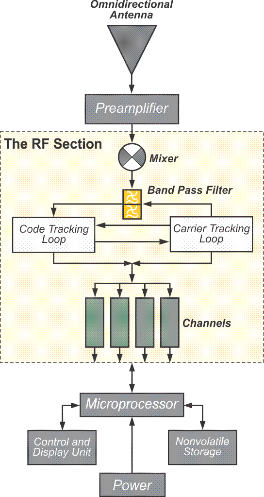
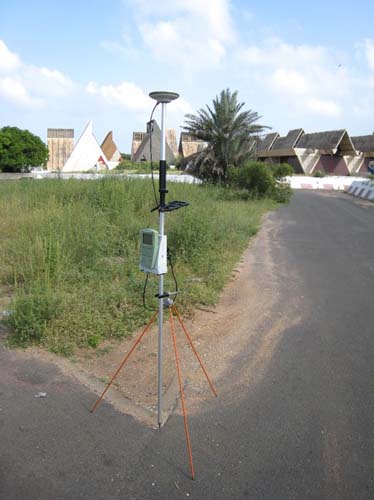
GPS receivers come in a variety of shapes and sizes. Some have external batteries, data collectors. Some are tripod mounted. Some are hand-held and have all components built in, and some can be used in both ways, with externals and without. Nevertheless, most have similar characteristics. Here is a schematic drawing of a GPS receiver. It includes some of the common components.
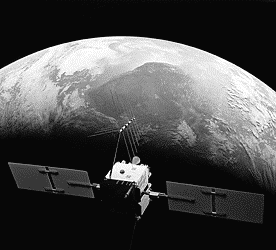
A GPS receiver must collect and then convert signals from GPS satellites into measurements of position, velocity, and time. There is a challenge in that the GPS signal has low power. An orbiting GPS satellite broadcasts its signal across a cone of approximately 28º of arc. From the satellite’s point of view, about 11,000 miles up, that cone covers a substantial portion of the whole planet. It is instructive to contrast this arrangement with a typical communication satellite that not only has much more power, but also broadcasts a very directional signal. Its signals are usually collected by a large dish antenna, but the typical GPS receiver has a small, relatively non-directional antenna. Stated another way, a GPS satellite spreads a low power signal over a large area rather than directing a high power signal at a very specific area. Fortunately, antennas used for GPS receivers do not have to be pointed directly at the signal source. The GPS signal also intentionally occupies a broader bandwidth than it must, to carry its information. This characteristic is used to prevent jamming and mitigate multipath but, most importantly, the GPS signal itself would be completely obscured by the variety of electromagnetic noise that surrounds us if it were not a spread spectrum coded signal. In fact, when a GPS signal reaches a receiver, its power is actually less than the receiver's noise level; fortunately, the receiver can still extract the signal and achieve unambiguous satellite tracking using the correlation techniques described earlier. To do this job, the elements of a GPS receiver function cooperatively and iteratively. That means that the data stream is repeatedly refined by the several components of the device working together as it makes its way through the receiver.
The Antenna and The Right Hand Circular Polarized Signal

The antenna, radio frequency (RF) section, filtering and intermediate frequency elements are in the front of a GPS receiver. The antenna collects the satellite’s signals and converts the incoming electromagnetic waves into electric currents sensible to the RF section of the receiver. Several antenna designs are possible in GPS, but the satellite’s signal has such a low power density, especially after propagating through the atmosphere, that antenna efficiency is critical. Therefore, GPS antennas must have high sensitivity, also known as high gain. They can be designed to collect only the L1 frequency, L1 and L2, or all signals, including L5. In all cases, they must be Right Hand Circular Polarized, (RHCP), as are the GPS signals broadcast from the satellites.
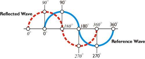
Polarized waves oscillate in more than one direction. The electrical field vectors of the GPS Signal have a constant magnitude, but their direction rotates so that the electrical field vector of the wave describes a helix in the direction of propagation. Said another way, circularly polarized waves are those where the angle of the electric vector rotates around an imaginary line traveling in the direction of the propagation of the wave. The rotation may be either to the right or left. The GPS signal is a Right-Hand Circularly Polarized (RHCP) wave. You can illustrate it this way. With your right hand, give the thumbs up signal. Now, instead of pointing your thumb up, point it in the direction that the GPS signal is propagating. Your curling fingers show you the direction of the rotation of the field.
The Antenna
Bottom left: Dipole antenna, Bottom right: Helix antenna
Top right: LEA
Bottom left: http://www.sciperio.com/antenna/antenna-design.asp
Bottom right: www.professionalwireless.com/helical/index.aspx
The illustration shows antenna types. They are not specifically GPS antennas.
Most receivers have an antenna built in, but many can accommodate a separate tripod-mounted or range pole-mounted antenna as well. These separate antennas sometimes require connecting coaxial cables. The cables are an important detail. The longer the cable, the more of the GPS signal is lost traveling through it. They are usually in standard lengths to make sure that the impedance of the trip through the cable can be calibrated.
As mentioned earlier, the wavelengths of the GPS carriers are 19 cm (L1), 24 cm (L2) and 25 cm (L5), and antennas that are a quarter or half wavelength tend to be the most practical and efficient, so GPS antenna elements can be as small as 4 or 5 cm. Most of the receiver manufacturers use a microstrip antenna. These are also known as patch antennas. The microstrip may have a patch for each frequency, so it can receive one or all of the GPS carriers. Microstrip antennas are durable, compact, have a simple construction and a low profile. The next most commonly used antenna is known as a dipole. You may recall that this is the kind of antenna that was used with the Macrometer, the first commercial GPS receiver. A dipole antenna has a stable phase center and simple construction, but needs a good ground plane. A ground plane also facilitates the use of a microstrip antenna where it not only ameliorates multipath, but also tends to increase the antenna’s zenith gain-- in other words, the gain of the antenna straight up. A quadrifilar antenna is a single frequency antenna that has two orthogonal bifilar helical loops on a common axis. Quadrifilar antennas perform better than a microstrip on crafts that pitch and roll, like boats and airplanes. They are also used in many recreational handheld GPS receivers. Such antennas have a good gain pattern, do not require a ground plane, but are not azimuthally symmetric. The least common design is the helix antenna. A helix is a dual frequency antenna. It has a good gain pattern, but a high profile.
Bandwidth
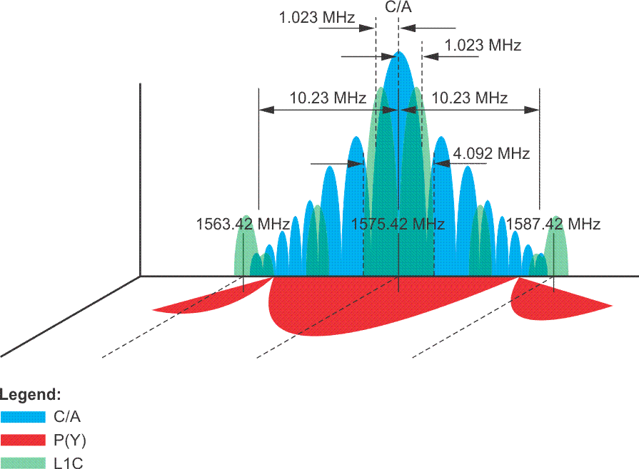
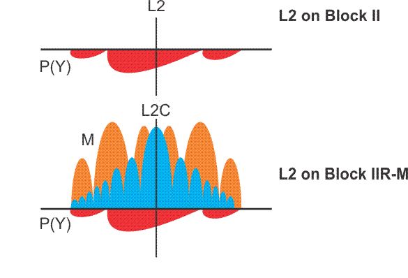
An antenna ought to have a bandwidth commensurate with its application. In general, the larger the bandwidth, the better the performance; however, there is downside. Increased bandwidth degrades the signal-to-noise ratio by including more interference. These PSD diagrams illustrate the C/A and P code signals power per bandwidth in Watts per Hertz as a function of frequency. GPS microstrip antennas usually operate in a range from about 2 to 20 MHz, which corresponds with the null-to-null bandwidth of the GPS signals. For example, the L2C signal, like the C/A, has the span of 2.046 megahertz. You can see it in the highest portion or the central lobe of the diagram. L5, like the P code, has a bandwidth of 20.46 megahertz, as you see in red. So an antenna on the front end of the receiver has to be able to accommodate that bandwidth of 20.46 megahertz if it is to track all of these signals. If the system's tracking C/A code or the L2C only, it could have a narrower bandwidth. It would need 2.046 MHz for the central lobe of the C/A code, or if it were designed to track the L1C signal, its bandwidth would need to be 4.092 MHz. A dual frequency microstrip antenna would likely operate in a bandwidth from 10 to 20 MHz.
Nearly Hemispheric Coverage
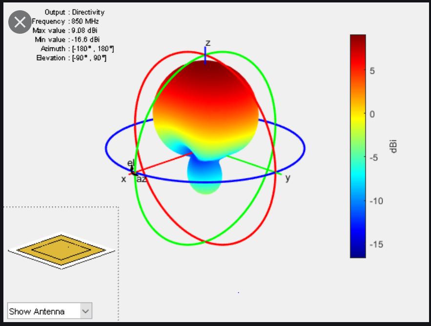
Since a GPS antenna is designed to be omnidirectional, its gain pattern, that is the change in gain over a range of azimuths and elevations, ought to be nearly a full hemisphere, but not perfectly hemispheric. For example, most surveying applications filter the signals from very low elevations to reduce the effects of multipath and atmospheric delays. A portion of the GPS signal may come into the antenna from below the mask angle; therefore, the antenna’s gain pattern is specifically designed to reject such signals. Second, the contours of equal phase around the antenna’s electronic center, that is, the phase center, are not themselves perfectly spherical.
The gain, or gain pattern, describes the success of a GPS antenna in collecting more energy from above the mask angle, and less from below the mask angle. A gain of about 3 to 5 decibels (dB) is typical for a GPS antenna. Just a brief description of a decibel-- we'll be seeing a little bit more of it. The decibel is a tenth of a bell, which was named for Alexander Graham Bell. It is a logarithmic dimensionless unit used to make a comparison. In this case, the gain of a real GPS antenna is compared to a theoretical lossless antenna that has perfectly equal capabilities in all directions. This imaginary perfection is known as an isotropic antenna. By the way a 3 decibel increase indicates a doubling of signal strength, and a 3 decibel decrease indicates a halving of signal strength so a typical omnidirectional GPS antenna with a gain of about 3 dB (decibels) has about 50% of the capability of that perfect isotropic antenna.
A decibel watt, dbW, indicates the actual power of a signal compared to a reference of one watt, The minimum power received from the C/A code on L1 is about -160dBW, -160 decibel Watts and the minimum power received from the P code on L2 is even less at -166 dBW. It is important that the GPS receiver antennas and pre-amplifiers be as efficient as possible, because the power received from the GPS satellites is low.
Antenna Orientation
In a perfect GPS antenna, the phase center of the gain pattern would be exactly coincident with its actual, physical, center. If such a thing were possible, the centering of the antenna over a point on the earth would ensure its electronic centering as well. But that absolute certainty remains elusive for several reasons.
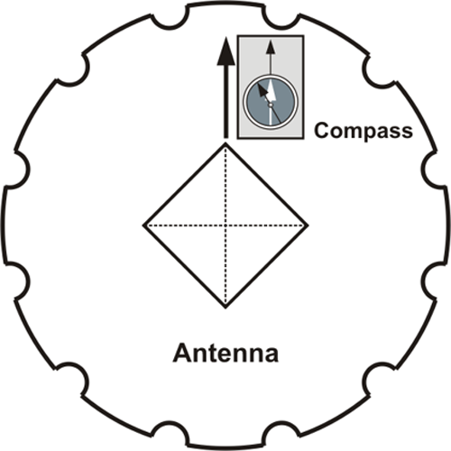
It is important to remember that the position at each end of a GPS baseline is the position of the phase center of the antenna at each end, not their physical centers, and the phase center is not an immovable point. The location of the phase center actually changes slightly with the satellite’s signal. For example, it is different for the L2 than for L1 or L5. In addition, as the azimuth, intensity, and elevation of the received signal changes, so does the difference between the phase center and the physical center. Small azimuthal effects can also be brought on by the local environment around the antenna. But most phase center variation is attributable to changes in satellite elevation. In the end, the physical center and the phase center of an antenna may be as much as a couple of centimeters from one another. On the other hand, with today’s patch antennas, it can be as little as a few millimeters. It is fortunate that the shifts are systematic. To compensate for some of this offset error, most receiver manufacturers recommend users make sure their antennas are all oriented in the same direction when making simultaneous observations on a network of points. Several manufacturers provide reference marks on the antenna, so that each one may be rotated to the same azimuth, usually north, to maintain the same relative position between their physical and phase, electronic, centers. By orienting all the antennas in the same direction, the offset between the phase center and the physical center is in the same direction at each point. Therefore, the baselines come out exactly as if the physical and the phase center were coincident.
It's only when we're talking about control work, work that needs to be quite accurate, that all of the antennas need to be oriented to the same direction.
Height of Instrument
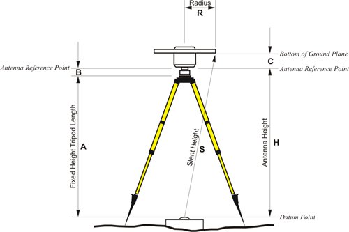
The antenna's configuration also affects another measurement critical to successful GPS work - the height of the instrument. An incorrect height of instrument is one of the most easily avoided errors. The measurement is normally made to some reference mark on the antenna. In this diagram, you see many ways of measuring that height. It can be measured at slant height or measured with a tape, usually to the antenna reference point. The ARP, or the antenna reference point, is frequently the bottom of the mount of the antenna. There's usually a correction to be added to actually bring that measurement up to the phase center of the antenna. This also becomes part of the necessary information when one is using continuously operating reference stations. We talked earlier about the fact that it is possible to take the downloads from NGS managed Continuously Operating Reference Station (CORS) stations that are available on the Internet and post-process the observations taken with a roving GPS receiver. If you are doing so, it is also necessary to know the height of the antenna at the CORS. Of course, that is not an antenna that you would've set up, but that information is available along with the files from the base station.
The RF Section
The pre-amplifier is necessary, because the signal coming in from the GPS satellite is weak. The preamplifier increases the signal’s power, but it is important that the gain in the signal coming out of the preamplifier is considerably higher than the noise. Noise is always part of the signal. Since signal processing is easier if the signals arriving from the antenna are in a common frequency band, the incoming frequency is combined with a signal at a harmonic frequency. This latter, pure sinusoidal signal is the previously mentioned reference signal generated by the receiver’s oscillator. The two frequencies are multiplied together in a device known as a mixer. Two frequencies emerge: one of them is the sum of the two that went in, and the other is the difference between them. The sum and difference frequencies then go through a bandpass filter, an electronic filter that removes the unwanted high frequencies and selects the lower of the two. It also eliminates some of the noise from the signal. For tracking the P(Y)-code, this filter will have a bandwidth of about 20 MHz, but it will be around 2 MHz if the C/A code is required. In any case, the signal that results is known as the intermediate frequency (IF), or beat frequency signal. This beat frequency is the difference between the Doppler-shifted carrier frequency that came from the satellite and the frequency generated by the receiver’s own oscillator. In fact, to make sure that it embraces the full range of the Doppler effect on the signals coming in from the GPS satellites, the bandwidth of the IF itself can vary from 5 to 10 kHz Doppler. That spread is typically lessened after tracking is achieved.
As mentioned before, a replica of the C/A or P(Y) code is generated by the receiver’s oscillator and that is correlated with the IF signal. It is at this point that the pseudorange is measured. Remember, the pseudorange is the time shift required to align the internally generated code with the IF signal, multiplied by the speed of light. The receiver also generates another replica, this time a replica of the carrier. That carrier is correlated with the IF signal and the shift in phase can be measured. The continuous phase observable, or observed cycle count, is obtained by counting the elapsed cycles since lock-on and by measuring the fractional part of the phase of the receiver generated carrier.
Channels
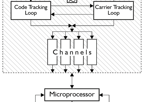
We're not talking about just receiving one signal from one satellite but rather a minimum of four, and perhaps many more, from four to more satellites and the antenna itself does not sort the information it gathers. The signals from several satellites enter the receiver simultaneously. But in the channels of the RF section, the undifferentiated signals are identified and segregated from one another. There are usually several IF stages before the copies are sent into the separate channels, each of which extract the code and carrier information from a particular satellite. A channel in a continuous tracking GPS receiver is not unlike a channel in a television set. It is hardware, or a combination of hardware and software, designed to separate one signal from all the others. A receiver may have 6 channels, 12 channels, or hundreds of channels. At any given moment, one frequency from one satellite can have its own dedicated channel, and the channels operate in parallel. This approach allows the receiver to maintain accuracy when it is on a moving platform; it provides anti-jamming capability and shortens the time to first fix (TTFF). Each channel typically operates in one of two ways; working to acquire the signal or to track it. Once the signal is acquired, it is continuously tracked unless lock is lost. If that happens, the channel goes back to acquisition mode and the process is repeated.
While a parallel receiver has dedicated separate channels to receive the signals from each satellite that it needs for a solution, a multiplexing (aka muxing) receiver gathers some data from one satellite and then switches to another satellite and gathers more data and so on. Such a receiver can usually perform this switching quickly enough that it appears to be tracking all of the satellites simultaneously. A multiplexing receiver must still dedicate one frequency from one satellite to one channel at a time; it just makes that time very short. It typically switches at a rapid pace, i.e., 50 Hz. Even though multiplexing is generally less expensive, this strategy of switching channels is now little used. There are several reasons. While a parallel receiver does not necessarily offer more accurate results, parallel receivers with dedicated channels are faster; a parallel receiver has a more certain phase lock; and there is redundancy if a channel fails and they possess a superior signal-to-noise ratio (SNR). A multiplexing receiver also has a lower resistance to jamming and interference compared to continuous tracking receivers. Whether continuous or switching channels are used, a receiver must be able to discriminate between the incoming signals. They may be differentiated by their unique C/A codes on L1, their Doppler shifts, or some other method, but, in the end, each signal is assigned to its own channel.
Tracking Loops
There are code tracking loops, the delay lock loops (DLL) and carrier tracking loops, and the phase locking loops (PLL) in the receiver. Typically, both the code and the carrier are being tracked in phase lock. The tracking loops connected to each of the receiver’s channels also work cooperatively with each other. As mentioned, dual frequency receivers have dedicated channels and tracking loops for each frequency.
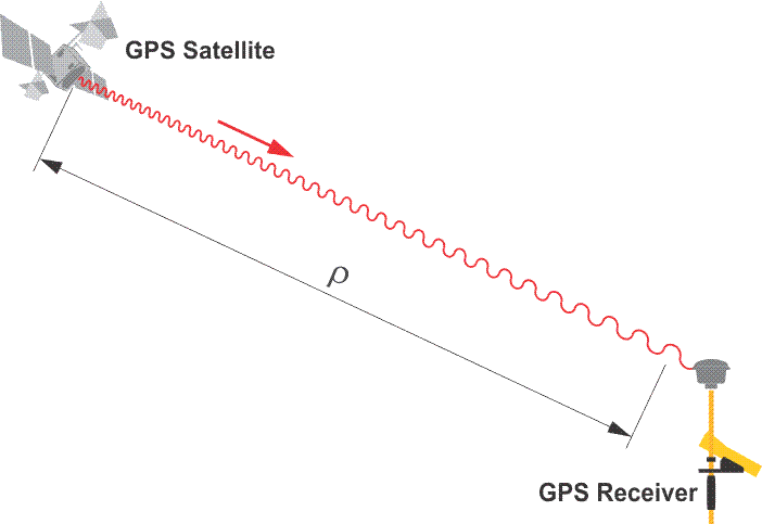
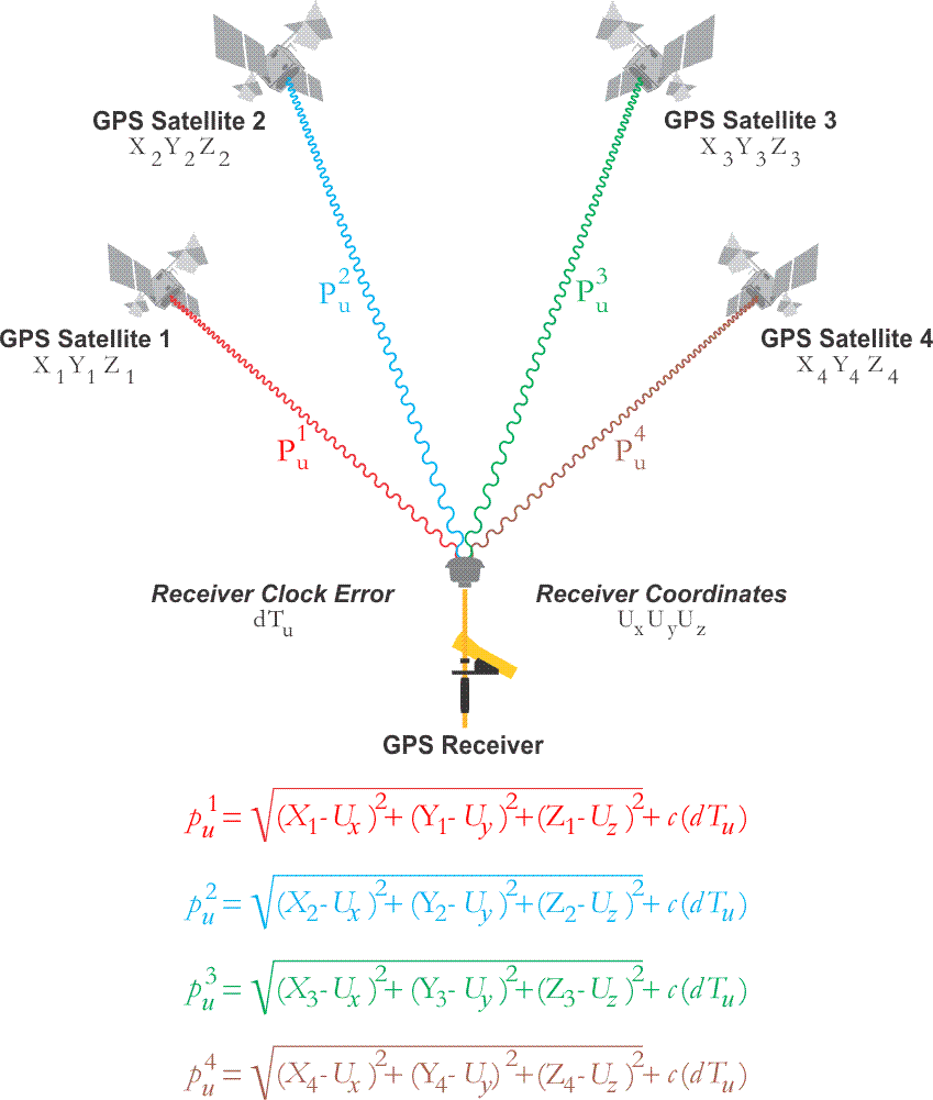
Pseudoranging
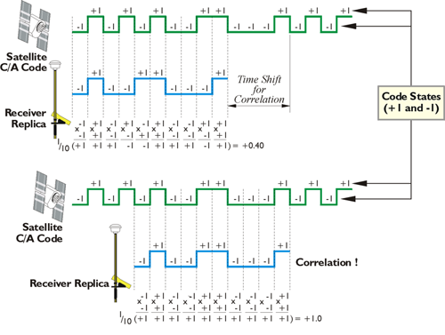
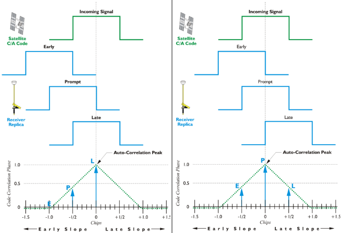
In most receivers, the first procedure in processing an incoming satellite signal is synchronization of the C/A code from the satellite’s L1 broadcast, with a replica C/A code generated by the receiver itself, i.e., the code-phase measurement. When there is no initial match between the satellite’s code and the receiver’s replica, the receiver time shifts, or slews, the code it is generating until the optimum correlation is found. Then a code tracking loop, the delay lock loop, keeps them aligned. The time shift discovered in that process is a measure of the signal’s travel time from the satellite to the phase center of the receiver’s antenna. Multiplying this time delay by the speed of light gives a range. But it is called a pseudorange in recognition of the fact that it is contaminated by the errors and biases set out in Lesson 2. The tracking loops that we see in the schematic diagram at the top are the code tracking loops.
Tracking loops are connected to each of the receiver's channels and also work cooperatively with each other. Multiple frequency receivers have dedicated channels and tracking loops for each frequency. Most receivers use the pseudorange range (the C/A code, on the L1) as the front door, so to speak, for the incoming satellite's synchronization. As we've discussed, the replica code is used to accomplish correlation. As you see in the diagram, the incoming signal is in the green at the top. The receiver replica is in blue. There is illustration of the replica as early, prompt, and late. When it is prompt, the replica and the incoming signal are correlated.
Carrier Phase Measurement
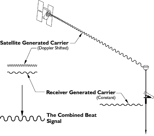
Once the receiver acquires the C/A code, it has access to the NAV message, or the newer navigation messages such as CNAV. It can read the ephemeris and the almanac information, use GPS time. But the code’s pseudoranges, alone, are not adequate for the majority of applications. Therefore, the next step in signal processing for most receivers involves the carrier phase observable. As stated earlier, just as they produce a replica of the incoming code, receivers also produce a replica of the incoming carrier wave. And the foundation of carrier phase measurement is the combination of these two frequencies. Remember, the incoming signal from the satellite is subject to an ever-changing Doppler shift, while the replica within the receiver is nominally constant.
Carrier Tracking Loop
The process begins after the PRN code has done its job and the code tracking loop is locked. By mixing the satellite’s signal with the replica carrier, this process eliminates all the phase modulations, strips the codes from the incoming carrier, and simultaneously creates two intermediate or beat-frequencies—one is the sum of the combined frequencies, and the other is the difference. The receiver selects the latter, the difference, with a bandpass filter. Then, this signal is sent on to the carrier tracking loop also known as the phase locking loop, PLL, where the voltage-controlled oscillator is continuously adjusted to follow the beat frequency exactly. This is basically how a GPS receiver locks on to that carrier and stays locked unless there is a loss of signal or a cycle slip.
Doppler Shift
We've talked about the Doppler shift in several different contexts. One was the original transit system, NNSS system, that operated on the Doppler shift. As the satellite passes overhead, the range between the receiver and the satellite changes; that steady change is reflected in a smooth and continuous movement of the phase of the signal coming into the receiver. GPS uses the Doppler shift as an observable. It has broad applications in signal processing. It can be used to discriminate between the signals from various GPS satellites, to determine integer ambiguities in kinematic surveying, as a help in the detection of cycle slips, and as an additional independent observable for autonomous point positioning. But perhaps the most important application of Doppler data is the determination of the range rate between a receiver and a satellite. Range rate is a term used to mean the rate at which the range between a satellite and a receiver changes over a particular period of time.
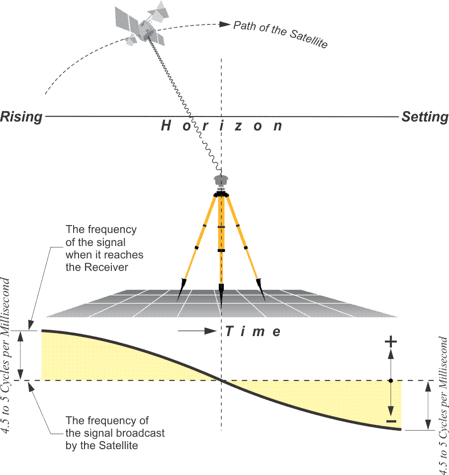
Typical Change in the Doppler Shift
This graphic shows the typical rate of change in the Doppler shift with regard to a stationary, static, GPS receiver. The signal received would have its maximum Doppler shift, +4 1/2 to 5 cycles per millisecond, when the satellite is at its maximum range, just as it is rising or setting. The Doppler shift continuously changes throughout the overhead pass. Immediately after the satellite rises, relative to a particular receiver, its Doppler shift gets smaller and smaller, until the satellite reaches its closest approach, at zenith. At that moment its radial velocity with respect to the receiver is zero, the Doppler shift of the signal is zero as well. But as the satellite recedes, it grows again, negatively, until the Doppler shift once again reaches its maximum extent just as the satellite sets, -4 1/2 to 5 cycles per millisecond. It is very predictable. That predictability, the constant variation of the signal's Doppler shift, makes it a good observable. If the receiver's oscillator frequency is adjusted to match these variations exactly, as they're happening, it will duplicate the incoming signal's shift and phase. This strategy of making measurements using the carrier beat phase observable is a matter of counting the elapsed cycles and adding the fractional phase of the receiver's own oscillator. This is one way that the phase lock loop maintains its lock on the signal as the Doppler shift occurs with each of the satellites that it is tracking.
With respect to the receiver, the satellite is always in motion even if the receiver is static. But the receiver may be in motion in another sense, as it is in kinematic GPS. The ability to determine the instantaneous velocity of a moving vehicle has always been a primary application of GPS, and is based on the fact that the Doppler-shift frequency of a satellite’s signal is nearly proportional to its range rate. The Doppler shift can be used to discriminate between the signals of the various satellites to help in the determination of the integer ambiguity. It can help in detection of a loss of lock due to a cycle slip.
Continuously Integrated Doppler
The Doppler-shift and the carrier phase are measured by first combining the received frequencies with the nominally constant reference frequency created by the receiver’s oscillator. The difference between the two is the often mentioned beat frequency, an intermediate frequency, and the number of beats over a given time interval is known as the Doppler count for that interval. Since the beats can be counted much more precisely than their continuously changing frequency can be measured, most GPS receivers just keep track of the accumulated cycles, the Doppler count. The sum of consecutive Doppler counts from an entire satellite pass is often stored, and the data can then be treated like a sequential series of biased range differences. Continuously Integrated Doppler is such a process. The rate of the change in the continuously integrated Doppler shift of the incoming signal is the same as that of the reconstructed carrier phase. Integration of the Doppler frequency offset results in an accurate measurement of the advance in carrier phase between epochs. And as stated earlier, using double-differences in processing the carrier phase observables removes most of the error sources other than multipath and receiver noise.
The Integer Ambiguity
The solution of the integer ambiguity, the number of whole cycles on the path from satellite to receiver, would be more difficult if it was not preceded by pseudoranges, or code phase measurements in most receivers. This allows the centering of the subsequent double-difference solution. In other words, a pseudorange solution provides an initial estimate of the candidates for the integer ambiguity within a smaller range than would otherwise be the case, and, as more measurements become available, it can reduce them even further. After the code-phase measurements narrows the field, there are several methods used to solve the integer ambiguity. In the geometric method, the carrier phase data from multiple epochs are processed, and the constantly changing satellite geometry is used to find an estimate of the actual position of the receiver. This approach is also used to show the error in the estimate by calculating how its results hold up as the geometry of the constellation changes. This strategy requires a significant amount of satellite motion to succeed, and, therefore, takes time to converge on a solution. It works pretty well, but requires satellite motion and takes time to converge. Another approach to solving the integer ambiguity is filtering. Independent measurements are averaged to find the estimated position with the lowest noise level. A third uses a search through the range of possible integer ambiguity combinations from which it calculates the one with the lowest residuals. These approaches can't assess the correctness of the particular answer, but they can provide the probability with certain conditions, that the answer is within given limits. Most GPS receivers use a combination of methods. Nearly all narrow the field by beginning with an initial position established by the code phase measurements. They then use one or more of the methods in combination to come up with the most probable value for the solution of the integer ambiguity, the N, the number of full wave cycles between the receiver and the satellite at lock on, the key to carrier phase observations.
Signal Squaring
There is a method that does not use the codes carried by the satellite’s signal. It is called codeless tracking, or signal squaring. It was first used in the earliest civilian GPS receivers, supplanting proposals for a TRANSIT-like Doppler solution. It makes no use of pseudoranging and relies exclusively on the carrier phase observable. Like other methods, it also depends on the creation of an intermediate or beat frequency. But with signal squaring, the beat frequency is created by multiplying the incoming carrier by itself. The result has double the frequency and half the wavelength of the original. It is squared. There are some drawbacks to the method. For example, in the process of squaring the carrier, it is stripped of all its codes. The chips of the P(Y) code, the C/A code, and the Navigation message normally modulated onto the carrier by 180° phase shifts are eliminated entirely. As discussed earlier, the signals broadcast by the satellites have phase shifts called code states that change from +1 to –1 and vice versa, but squaring the carrier converts them all to exactly 1. The result is that the codes themselves are wiped out. Therefore, this method must acquire information such as almanac data and clock corrections from other sources. Other drawbacks of squaring the carrier include the deterioration of the signal-to-noise ratio, because when the carrier is squared, the background noise is squared, too. And cycle slips occur at twice the original carrier frequency. But signal squaring has its up-side as well. It reduces susceptibility to multipath. It has no dependence on PRN codes and is not hindered by the encryption of the P code. The technique works as well on L2 as it does on L1 or L5, and that facilitates ionospheric delay correction. Therefore, signal squaring can provide high accuracy over long baselines. So, there is a cursory look at some of the different techniques used to process the signal in the RF section. Now let's look at the microprocessor of the receiver.
The Microprocessor
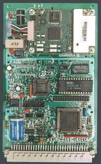
The microprocessor in a GPS receiver is the computer that manages data collection and is the home of the applications that mitigate multipath, noise, extract the ephemerides and other information from the Navigation message or newer navigation messages such as CNAV. It controls the entire receiver: the digital circuits, the tracking, and measurements. The receiver also has storage. However, more and more, the microprocessor is expected to produce the position in real time, instantaneously, or near real-time by processing the ranging data, doing reference frame (datum) conversion, and sending the position to the control and display unit (CDU). There is a two-way street between the microprocessor and the CDU; each can receive information from or send information to the other.
Differential Positioning
Autonomous single-point positioning using unsmoothed code pseudoranges are based upon corrections provided in the navigation messages, which, as you know, have a certain amount of weakness. Though they have improved since Selective Availability has been switched off, they are generally not as accurate as differentially corrected positions. Code-based pseudoranges using DGPS, differential GPS, can achieve good real-time, or post-processed results. DGPS is often used in collecting data for Geographical Information Systems, GIS.
DGPS
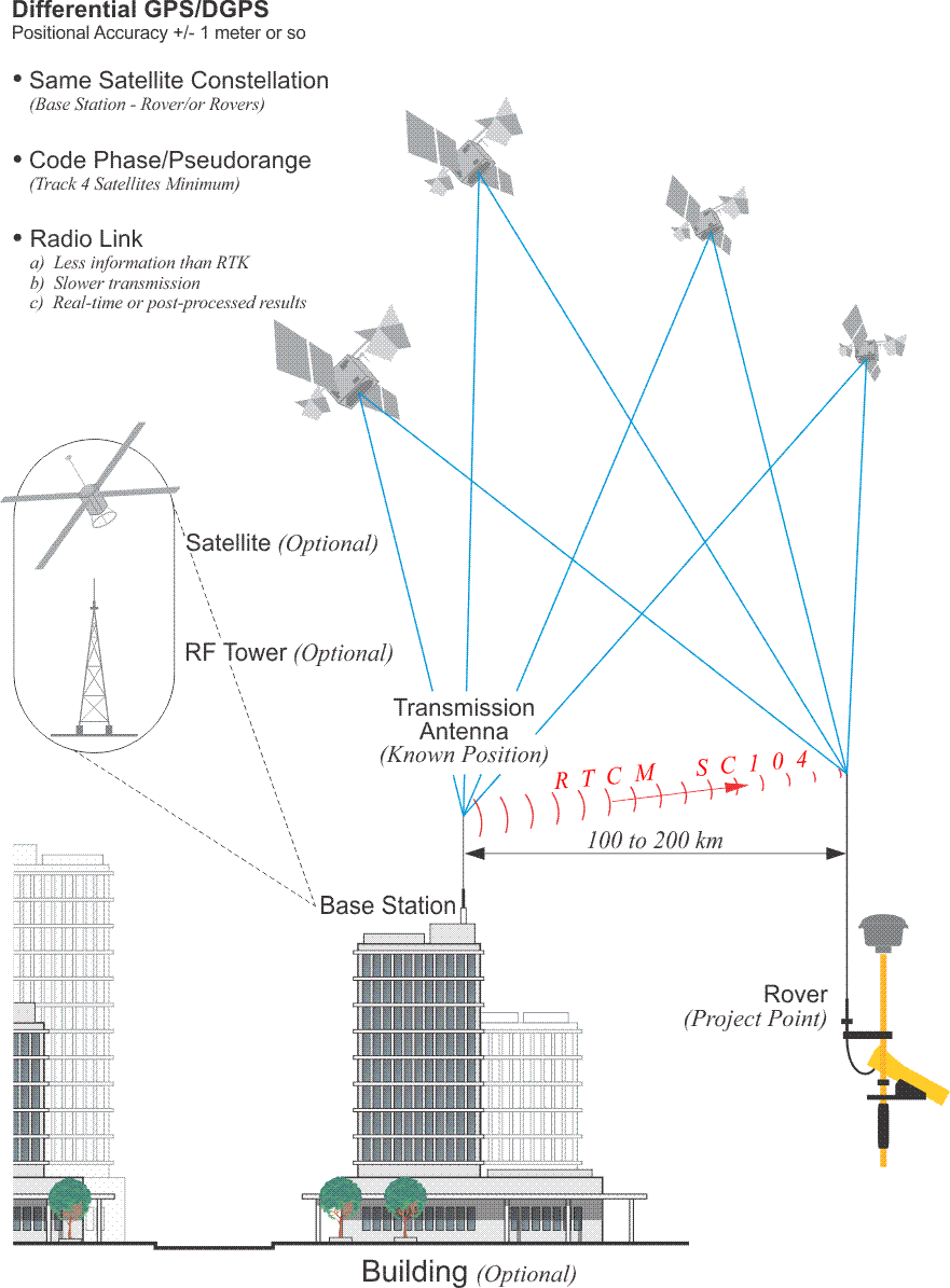
The type of differential positioning sometimes known as DGPS depends on code pseudorange observations, but requires at least two receivers. One receiver is placed on a control station, the base, and another on an unknown position, the rover. The base station antenna needn't be on a building, as illustrated. It could be on a tower. It could be on a non-GPS satellite. There are services that allow you to subscribe to a correction signal. In those cases, there is a network of base stations collecting the signals from the constellation; the correction signal is compiled, beamed up to the non-GPS satellite, and that same message sent back down from the non-GPS satellite to subscribers. In all configurations, the base and the rover simultaneously receive the same signals from the same constellation of at least four GPS/GNSS satellites. That's important in that the way many of the errors in the observations are common to both the base and the rover receivers, the errors are correlated and tend to cancel each other to some degree. The data from such an arrangement can be post-processed; although, with a link between the base and the rover, a correction signal can be sent to the rover so that differential results can be had in real-time. Improvements in this technology have refined the technique's accuracy markedly, and meter- or even submeter results are possible. Still, the positions are not as reliable as those achieved with the carrier phase observable.
With GIS, corner search and mapping work excepted, much GPS work requires a higher standard of accuracy. Certainly, GPS control surveying often employs several static receivers that simultaneously collect and store carrier phase data from the same satellites for a period of time known as a session. After all the sessions for a day are completed, their data are usually downloaded in a general binary format to the hard disk of a PC for post-processing. However, carrier phase positioning can also be done in real-time.
Real-Time Kinematic
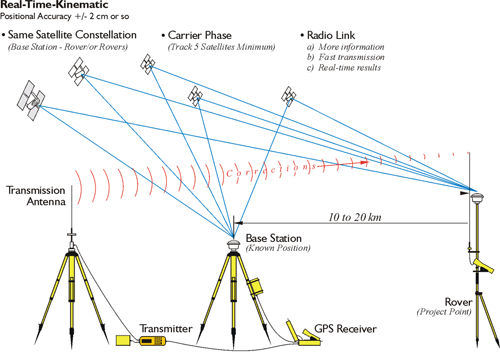
Real-time kinematic surveying uses the carrier phase solution. Often, there is a radio link between the base and rover. While the baseline length with DGPS is often 100 to 200 kilometers or longer, the baseline length in RTK is more typically 10 to 20 kilometers, often less. However, the arrangement of receivers is similar: the constellation of satellites being tracked at the base station and also tracked at the rover, the base station is at a known point. There is a transmission antenna used in RTK. It transmits the correction signals to the rover in real time correction. While the arrangement is similar to DGPS, the solution is carrier phase as opposed to pseudorange. The minimum number of satellites with RTK is five. It is five, so that one can be lost and still assured that there will be a solution.
The CDU
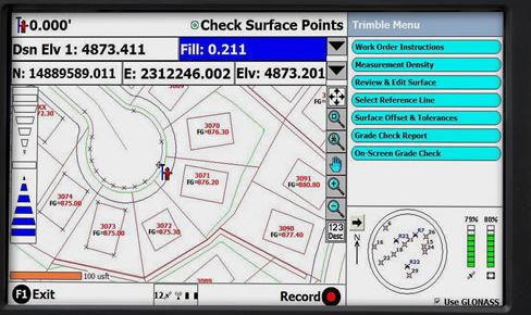
A GPS receiver will often have a control and display unit. From handheld keyboards to soft keys around a screen to digital map displays and interfaces to other instrumentation, there are a variety of configurations. Nevertheless, they all have the same fundamental purpose, facilitation of the interaction between the operator and the receiver’s microprocessor. A CDU typically displays status, position data, velocity, and time. It may also be used to select different surveying methods, waypoint navigation, and/or set parameters such as epoch interval, mask angle, and antenna height. The CDU can offer a combination of help menus, prompts, reference frame (datum) conversions, readouts of survey results, estimated positional error, and so forth. The information available from the CDU varies from receiver to receiver. But when four or more satellites are available, they can generally be expected to display the PRN numbers of the satellites being tracked, the receiver’s position in three dimensions, and velocity information. Most of them also display the dilution of precision and GPS time or UTC.
The Storage


Most GPS receivers today have internal data logging. The amount of storage required for a particular session depends on several things: the length of the session, the number of satellites above the horizon, the epoch interval, and so forth. For example, presuming the amount of data received from a single GPS satellite is ~100 bytes per epoch, a typical twelve channel dual-frequency receiver observing 6 satellites and using a 1-second epoch interval over the course of a 1-hour session would require ~2MB of storage capacity for that session. The miniaturization of storage continues. The cassettes, floppy disks, and drives used with the Macrometer are past. Extraordinary amounts of data can be stored in small, convenient devices or sent to the cloud.
The Power
Battery power
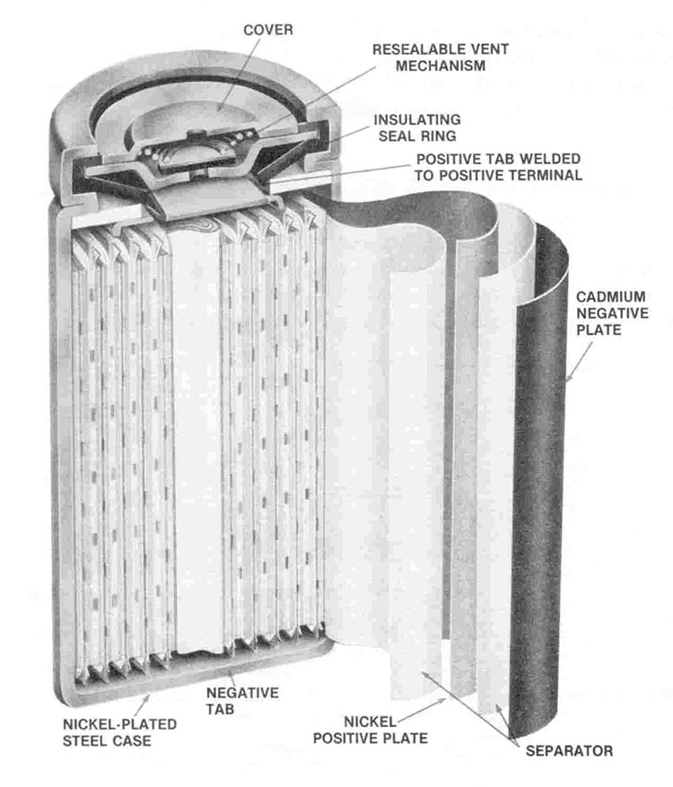
It is fortunate that GPS receivers operate at low power. From 9 to 36 volts DC is generally required. This allows longer observations with fewer, and lighter, batteries than might be otherwise required. It also increases the longevity of the GPS receivers, themselves. About half of the available GPS carrier phase receivers have an internal power supply, and most will operate 5½ hours or longer on a fully charged 6-amp-hour battery. Most code-tracking receivers, those that do not also use the carrier phase observable, could operate for about 15 hours on the same size battery. Since most receivers in the field operate on battery power, batteries and their characteristics are fundamental to GPS/GNSS. A variety of batteries are used, and there are various configurations. For example, some units are powered by rechargeable batteries. Lithium, Nickel Cadmium, and Nickel Metal-Hydride may be the most common categories, but lead-acid car batteries still have an application as well. The obvious drawbacks to lead-acid batteries are size and weight. And there are a few others—the corrosive acid, the need to store them charged, and their low cycle life. Nevertheless, lead-acid batteries are especially hard to beat when high power is required. They are economical and long-lasting.
Nickel Cadmium batteries (NiCd) cost more than lead-acid batteries, but are small and operate well at low temperatures. Their capacity does decline as the temperature drops. Like lead-acid batteries, NiCd batteries are quite toxic. They self-discharge at the rate of about 10% per month, and even though they do require periodic full discharge, these batteries have an excellent cycle life. Nickel Metal-Hydride (NiMH) batteries self-discharge a bit more rapidly than NiCd batteries and have a less robust cycle life, but are not as toxic. Lithium–ion batteries overcome several of the limitations of the others. They have a relatively low self-discharge rate. They do not require periodic discharging and do not have a memory issues as do NiCd batteries. They are light, have a good cycle life and low toxicity. On the other hand, the others tolerate overcharging, and the lithium-ion battery does not. It is best to not charge lithium-ion batteries at temperatures at or below freezing. These batteries require a protection circuit to limit current and voltage, but are widely used in powering electronic devices, including GPS/GNSS receivers.
Some GPS Surveying Methods
Static GPS surveying was the first method of GPS surveying used in the field, and it continues to be the primary technique for GPS/GNSS control today. Relative static positioning involves several stationary receivers simultaneously collecting data from at least four satellites during observation sessions that usually last from 30 minutes to 2 hours. A typical application of this method would be the determination of vectors, or baselines as they are called, between several static receivers to accuracies from 1 ppm to 0.1 ppm over tens of kilometers. There are few absolute requirements for relative static positioning. The requisites include: more than one receiver, four or more satellites, and a mostly unobstructed sky above the stations to be occupied. But, as in most of surveying, the rest of the elements of the system are dependent on several other considerations.
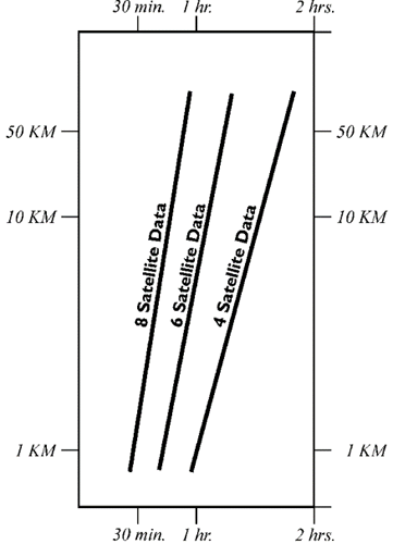
Here is a diagram of approximate session lengths required for GPS static surveying. For example, with an eight satellite constellation and a 10 kilometer baseline, something between a half an hour and an hour would typically be required. A four satellite constellation might require a session between one and two hours for a baseline of the same length. The assessment of the productivity of a GPS survey almost always hinges, in part at least, on the length of the observation sessions required to satisfy the survey specifications. The determination of the session's duration depends on several particulars, such as the length of the baseline and the relative position, that is the geometry, of the satellites among others. Generally speaking, the larger the constellation of satellites, the better the available geometry, the lower the positioning dilution of precision (PDOP), and the shorter the length of the session needed to achieve the required accuracy. For example, given six satellites and good geometry, baselines of 10 km or less might require a session of 45 minutes to 1 hour, whereas, under exactly the same conditions, baselines over 20 km might require a session of 2 hours or more. Alternatively, 45 minutes of six-satellite data may be worth an hour of four-satellite data, depending on the arrangement of the satellites in the sky.
Relative static positioning, just as all the subsequent surveying methods discussed here, involves several receivers occupying many sites. Problems can be avoided as long as the receivers on a project are compatible. For example, it is helpful if they have the same number of channels and signal processing techniques. The subject comes up from time to time as to whether or not data from receivers from various manufacture can be used on the same project together at the ends of even the same baseline. The answer is, yes of course because fortunately, there is a file format, that allows one to use receivers of many types together. It is the Receiver Independent Exchange Format, RINEX , developed by the Astronomical Institute of the University of Berne in 1989. It allows different receivers and post-processing software to work together. Almost all GPS/GNSS processing software will output RINEX files.
Receiver Categories
- Recreation Receivers
- Mapping Receivers
- Surveying Receivers
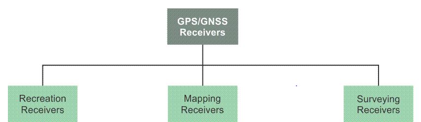
Receivers are generally categorized by their physical characteristics, the elements of the GPS signal they can use with advantage, and by the claims about their accuracy. There are receivers that use only the C/A code on the L1 frequency and receivers that cross-correlate with the P(Y) There are L1 carrier phase tracking receivers, dual-frequency and multi-frequency carrier phase tracking receivers, receivers that track all in view, and GPS/GNSS receivers. The more aspects of the GPS signal a receiver can employ, the greater its flexibility, but so, too, the greater its cost. It is important to understand receiver capabilities and limitations to ensure that the systematic capability of a receiver is matched to the required outcome of a project. As shown in the illustration, it is possible to divide receivers into three categories. They are; recreation, mapping, and surveying.
Recreational Receivers
| Recreational receivers | Autonomous Horizontal Precision |
Real-time Corrected Horizontal Network Accuracy |
Post-processed Horizontal Network Accuracy |
|---|---|---|---|
| Recreation | 5 - 15 m | 2 - 5 m | 5 - 15 m |
Recreation Receivers
These receivers are generally defined as L1 Code receivers which are typically not user configurable for settings such as mask angle, PDOP, the rate at which measurements are downloaded, the logging rate, also known as the epoch interval, and signal to noise ratio SNR. As you might expect, SNR is the ratio of the received signal power to the noise floor of a GPS observation. It is typical for the antenna, receiver, and CDU to be integrated into the device in these receivers. Generally speaking, receivers that track the C/A code provide only relatively low accuracy. Most are not capable of tracking the carrier phase observable. These receivers were typically developed with basic navigation in mind. Most are designed for autonomous (stand-alone) operation to navigate, record tracks, waypoints, and routes aided by the display of onboard maps. They are sometimes categorized by the number of waypoints they can store. Waypoint is a term that grew out of military usage. It means the coordinate of an intermediate position a person, vehicle, or airplane must pass to reach a desired destination. With such a receiver, a user may call up a distance and direction from his present location to the next waypoint.
A single receiver operating without augmentation produces positions which are not relative to any ground control, local or national. In that context, it is more appropriate to discuss the precision of the results than it is to discuss accuracy. Despite the limitations, some recreational receivers have capabilities that enhance their systematic precision and achieve a quantifiable accuracy using correction signals available from earth-orbiting satellites such as the Wide Area Augmentation System, WAAS correction. In other words, some have differential capability. The Wide Area Augmentation System is a U.S. Federal Aviation Authority FAA and the U.S. Department of Transportation DOT system that augments GPS accuracy, availability, and integrity. The system relies on a network of ground-based reference stations at known positions that observe the GPS constellation constantly. From their data, a correction message is calculated at two master stations. This message is uploaded to satellites on geostationary orbits. The satellites broadcast the message, and WAAS-enabled receivers can collect it and use the correction provided in it. For example, it provides a correction signal for precision approach aircraft navigation. Similar systems are Europe’s European Geostationary Navigation Overlay System, EGNOS, and Japan’s Multifunction Transport Satellite, MTSAT.
Recreational grade receivers typically do not have on-board feature data collection capabilities. They also do not usually have adequate on-board storage for recording the features (coordinates and attributes) required for a mapping project. Such capabilities are not needed for their designed applications. When a recreation receiver is used to obtain an autonomous, or stand alone, position, its precision may be within a range of 5-15m, as noted in Table 4.1. Under less than optimal field conditions: tree cover and other obstructions, less than favorable GPS satellite geometry, etc., users can expect the precision of autonomous positions to lessen, sometimes substantially. The network accuracy had with real-time differential correction of 2-5m is also not always achievable due to the tendency of the Wide Area Augmentation Signal being difficult to acquire, particularly in the northern US and then only with a southern sky clear of obstruction.
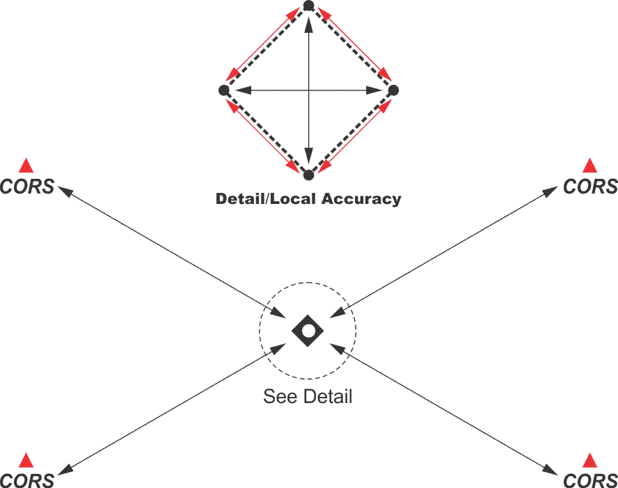
Local and Network Accuracy
Local and Network Accuracy
The use of the phrase network accuracy is used to define its difference from local accuracy. Network accuracy, here, concerns the uncertainty of a position relative to a reference frame (datum). Local accuracy is not about a position relative to a reference frame (datum), but it represents the uncertainty of a position relative to other positions nearby. In other words, local accuracy would be useful in knowing the accuracy of a line between the two positions at each end. Network accuracy would not be about the accuracy of the positions at each end of the line relative to each other, but, rather, relative to the whole reference frame (datum). Local Accuracy is also known as relative accuracy, and network accuracy is also known as absolute accuracy.
Within a well-defined geographical area, local accuracy may be the most immediate concern. However, those tasked with constructing a control network that embraces a wide geographical scope will most often need to know the position's relationship to the realization of the reference frame (datum) on which they are working. A point with good local accuracy may not have good network accuracy. Typically, network horizontal and vertical accuracies require that a point's accuracy be specified with respect to an appropriate national geodetic datum. In the United States, as a practical matter, this most often means that the work is tied to at least one of the Continuously Operating Reference Stations (CORS) which represent the most accessible realization of the National Spatial Reference System (NSRS) in the nation.
Mapping Receivers
| Mapping Receivers | Autonomous Horizontal Precision |
Real-time Corrected Horizontal Network Accuracy |
Post-processed Horizontal Network Accuracy |
|---|---|---|---|
| Mapping (L1 Code) | 2 - 10m | 0.5 - 5m | 0.3 - 15m |
| Mapping (L1 Code & Carrier) | 2 - 10m | 0.5 - 3m | 0.2 - 1m |
| Mapping (All GPS Code & Carrier) | 2 - 10m | 0.5 - 3m | 0.02 - 0.9m |
| Mapping (GNSS) | 2 - 10m | 0.5 - 3m | 0.02 - 0.9m |
Mapping Receivers
These receivers are generally defined as those that allow the user to configure some settings such as PDOP, SNR (carrier-to-noise-density ratio C/N0), elevation mask and the logging rate. They most often have an integrated antenna and CDU in the receiver. They generally record pseudoranges and also can log data suitable for differential corrections either in real-time or for post-processing; many record carrier data. Mapping receivers are often capable of storing mapped features (coordinates and attributes) and usually have adequate capacity for mapping applications. This memory is required for differential GPS, DGPS receivers, even those that track only code. For many applications, a receiver must be capable of collecting the same information as is simultaneously collected at a base station, and storing it for post-processing. Receivers typically depend on proprietary post-processing software, which also includes utilities to enable GPS data to be transferred to a PC and exported in standard GIS file format(s) either over a cable or a wireless connection. Some mapping grade receivers for spatial data collection are single frequency with code only or both code and carrier. Most mapping grade receivers of all tracking configurations are WAAS (or other Satellite Based Augmentation Signal SBAS) enabled, and thereby offer real-time results. Such differentially corrected mapping receivers may be capable of achieving a network accuracy of ~0.5 to 5 meters. Positions of sub-meter post-processed network accuracy can be achieved with mapping grade receivers. As noted, some mapping receivers offer tracking of the Global Navigation Satellite System, GNSS, constellations.
GNSS
Click here to see a text description.
GNSS
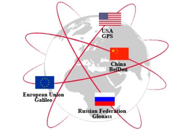
As mentioned earlier, the Global Positioning System (GPS) is now a part of a growing international context—the Global Navigation Satellite System (GNSS). One definition of GNSS embraces any constellation of satellites providing signals from space that facilitate autonomous positioning, navigation, and timing on a global scale. Currently, there are four systems that satisfy this definition. It is the Russian Federation’s GLONASS, European Union's GALILEO, China's BEIDOU and America's GPS.
There are several other regional satellite position, navigation and timing systems such as the Indian Regional Navigation Satellite System (IRNSS) and the Japanese Quasi-Zenith Satellite System (QZSS).
Surveying Receivers
| Survey Receivers | Autonomous Horizontal Precision |
Real-time Corrected Horizontal Network Accuracy |
Post-processed Horizontal Network Accuracy |
|---|---|---|---|
| Survey | 2 - 10 m | > 1 m | > 0.1 m |
Surveying Receivers
Survey grade receivers are designed for the achievement of consistent network accuracy in the static or real-time mode. Positions determined by these receivers will generally provide the best accuracy of the categories listed. The components of these receivers can usually be configured in a variety of ways. The receivers are typically multi-frequency, code and carrier receivers. Many are GNSS receivers. They generally provide more options for setting the observational parameters than recreational or mapping receivers. Surveying receivers are typically capable of observing the civilian code and carrier phase of all frequencies, and are appropriate for collecting positions on long baselines. Survey grade receivers are capable of producing network accuracies of better than 1 m with real-time differential correction and better than 0.1 m with post-processing.
Most share some practical characteristics: they have multiple independent channels that track the satellites continuously, and they begin acquiring satellites’ signals from a few seconds to less than a minute from the moment they are switched on. Most acquire all the satellites above their mask angle in a very few minutes, with the time usually lessened by a warm start, and most provide some sort of alert to the user that data is being recorded, and so forth. About three-quarters of them can have their sessions preprogrammed in the office before going to their field sites. Nearly all allow the user to select the logging rate, also known as epoch interval and also known as sampling interval. While a 1 second interval is often used, faster rates of 0.1 second (10 Hz) and more increments of tenths of a second are often available. This feature allows the user to stipulate the short period of time between each of the microprocessor's downloads to storage. The faster the data-sampling rate, the larger the volume of data a receiver collects, and the larger the amount of storage it needs. A fast rate is helpful in cycle slip detection, and that improves the receiver’s performance on baselines longer than 50 km, where the detection and repair of cycle slips can be particularly difficult.
Discussion
Discussion Instructions
To continue the discussion begun by this lesson, I would like to pose this question:
What are differences between differential GPS, static or kinematic, and autonomous (non-differential) GPS? Does differential GPS have to be post-processed?
To participate in the discussion, please go to the Lesson 4 Discussion Forum in Canvas. (That forum can be accessed at any time by going to the GEOG 862 course in Canvas and then looking inside the Lesson 4 module.)
Summary
The receivers and methods of GPS are constantly evolving and changing. There are, nevertheless, some well established principles. Some of those have been explained in this lesson.
There is another principle. GPS/GNSS is a geodetic system. It is not possible to understand it without some understanding of geodesy - the subject of the next lesson. As a matter of fact, it isn’t hard to operate a GPS/GNSS receiver - most of them are so user-friendly you don’t need to know the first thing about GPS/GNSS to make them work, that is, until they don’t.
Getting coordinates from a GPS/GNSS receiver is usually a matter of pushing a few buttons, but knowing what those coordinates are, and more importantly, what they aren’t, is more difficult. It is vital to have an idea of how the values were measured; otherwise you are at the mercy of the black box, and since it doesn’t always tell the truth, that’s not a good idea.
Before you go on to Lesson 5, double-check the Lesson 4 Checklist to make sure you have completed all of the activities listed there.