Lesson 7: Static Global Positioning System Surveying
The links below provide an outline of the material for this lesson. Be sure to carefully read through the entire lesson before returning to Canvas to submit your assignments.
Lesson 7 Overview
Overview
Static GPS/GNSS, where the receiver is stationary, is the original GPS/GNSS method. It is still the preferred approach for establishing the most accurate positions, the control. In many ways. For example, some processing and data checking should be performed on a daily basis during a GPS/GNSS project. Blunders from operators, noisy data, and unhealthy satellites can corrupt entire sessions. In any case, left undetected, such dissolution can jeopardize an entire project. These weaknesses in the data can sometimes be prevented before they happen by best practices such as optimization of the observation schedule. GPS/GNSS measurements are still composed of fundamentally biased ranges. Therefore, the goal remains to mitigate the biases and extract the true ranges. In this lesson, we start to get into the real details of how static GPS/GNSS work is done.
Objectives
At the successful completion of this lesson, students should be able to:
- discuss the difference between precision and accuracy
- discuss the basics of planning a static GPS/GNSS survey;
- recognize the role of NGS control;
- explain Continuously Operating Reference Stations;
- explain Static GPS/GNSS project design;
- demonstrate drawing GPS/GNSS baselines
- describe the difference between dependent and independent baselines;
- describe how to calculate the number of sessions necessary for a static survey;
- discuss some of the components of Static GPS/GNSS control such as equipment, station data sheets, visibility diagrams, monumentation and logistics
Questions?
If you have any questions now or at any point during this week, please feel free to post them to the Lesson 7 Discussion Forum. (To access the forum, return to Canvas and navigate to the Lesson 7 Discussion Forum in the Lesson 7 module.) While you are there, feel free to post your own responses if you, too, are able to help out a classmate.
Checklist
Lesson 7 is one week in length. (See the Calendar in Canvas for specific due dates.) To finish this lesson, you must complete the activities listed below. You may find it useful to print this page out first so that you can follow along with the directions.
| Step | Activity | Access/Directions |
|---|---|---|
| 1 | Read the lesson Overview and Checklist. | You are in the Lesson 7 online content now. The Overview page is previous to this page, and you are on the Checklist page right now. |
| 2 | Read Chapter 6 in GPS for Land Surveyors. | Text |
| 3 | Read the lecture material for this lesson. | You are currently on the Checklist page. Click on the links at the bottom of the page to continue to the next page, to return to the previous page, or to go to the top of the lesson. You can also navigate the lecture material via the links in the Lessons menu. |
| 4 | Participate in the Discussion. | To participate in the discussion, please go to the Lesson 7 Discussion Forum in Canvas. (That forum can be accessed at any time by going to the GEOG 862 course in Canvas and then looking inside the Lesson 7 module.) |
| 5 | Write a 2,400 word paper on one topic covered in the course over the previous weeks. | Please submit your paper to the Lesson 7 Paper Drop Box located in the Lesson 7 module. View Calendar in Canvas for specific due date. |
| 6 | Read lesson Summary. | You are in the Lesson 7 online content now. Click on the "Next Page" link to access the Summary. |
Static GPS Control Surveying
Static GPS/GNSS surveying has been used on control surveys from local to statewide to continental extent, and will probably continue to be the preferred technique in those categories. In static GPS/GNSS surveying, the receivers is motionless for a time, usually a relatively long occupation. If a static GPS/GNSS control survey is carefully planned, it usually progresses smoothly. The technology has virtually conquered two stumbling blocks that have defeated the plans of conventional surveyors for generations. Inclement weather does not disrupt GPS/GNSS observations, and a lack of intervisibility between stations is of no concern whatsoever, at least in postprocessed GPS/GNSS. Still, GPS/GNSS is far from so independent of conditions in the sky and on the ground that the process of designing a survey can now be reduced to points-per-day formulas, as some would like. Even with falling costs, the initial investment in GPS/GNSS remains large by most surveyors’ standards. However, there is seldom anything more expensive in a GPS/GNSS project than a surprise.
Planning a Static GPS/GNSS Control Survey: Accuracy and Precision
A Few Words about Accuracy
When planning a GPS/GNSS survey, one of the most important parameters is the accuracy specification. A clear accuracy goal avoids ambiguity both during and after the work is done. First, it is important to remember that there is a difference between precision and accuracy. One aspect of precision can be visualized as the tightness of the clustering of measurements; the closer the grouping, the more precise the measurement. Accuracy, on the other hand, requires one more element. It has to have a truth set. For example, the truth in illustration for A, B and C is the center of the target - without that accuracy is indefinable. In other words, accuracy is not determined by measurement alone. There must also be a standard value or values involved is through the comparison of the measurements with such standard values that the outcome of the work can be found to be sufficiently near the ideal or true value, or not.
For example, on the left in the illustration it may seem at first that the average of the measurements in the GPS-A group are more accurate than the average of those in GPS-B because the GPS-A group is more precise. However, when the true position is introduced on the right it is revealed that the GPS-B group’s average is the more accurate of the two, because accuracy and precision are not the same. When it comes to accuracy, there are other important details too. Local accuracy and network accuracy are not the same. As mentioned earlier, local accuracy, also known as relative accuracy, represents the uncertainty in the positions relative to the other adjacent points to which they are directly connected. Network accuracy, also known as absolute accuracy, requires that a position’s accuracy be specified with respect to an appropriate truth set such as a national geodetic datum. Differentially corrected GPS/GNSS survey procedures which are tied to CORS stations, which represent the National Spatial Reference System of the United States, provide information from which network accuracy can be derived. However, autonomous GPS/GNSS positioning, that is a single receiver without augmentation is not operating relative to any control, local or national. In that context, it is more appropriate to discuss the precision of the results than it is to discuss accuracy.
It is typical for uncertainty in horizontal accuracies to be expressed in a number that is radial. The uncertainties in vertical accuracies are given similarly, but they are linear, not radial. In both cases, the limits are always plus or minus (±). In other words, the reporting standard in the horizontal component is the radius of a circle of uncertainty, such that the true location of the point falls within that circle at some level of reliability, i.e. 95-percent of the time. Also, the reporting standard in the vertical component is a linear uncertainty value, such that the true location of the point falls within ± of that linear uncertainty to some degree of reliability. GPS positioning it is reasonable to expect that the vertical accuracy will be about 1/3 that of horizontal accuracy. If the absolute horizontal accuracy of a GPS position is ±1m then the estimate of the absolute vertical accuracy of the same GPS position would be ~±3m.
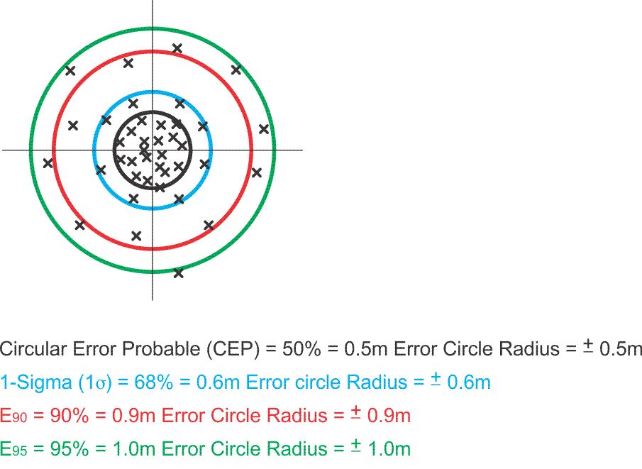
Here is a bit more on horizontal accuracy. The illustration shows a spread of positions around a center of the range. As the radius of the error circle grows larger, the certainty that the center of the range is the true position increases (it never reaches 100%).
It is not correct to say that every job suddenly requires the highest achievable accuracy, nor is it correct to say that every GPS/GNSS survey now demands an elaborate design. In some situations, a crew of two, or even one surveyor on-site may carry a GPS/GNSS survey from start to finish with no more planning than minute-to-minute decisions can provide, even though the basis and the content of those decisions may be quite different from those made in a conventional survey.
In areas that are not heavily treed and generally free of overhead obstructions, sufficient accuracy may be possible without a prior design of any significance. But while it is certainly unlikely that a survey of photocontrol or work on a cleared construction site would present overhead obstructions problems comparable with a static GPS/GNSS control survey in the Rocky Mountains, even such open work may demand preliminary attention. For example, just the location of appropriate vertical and horizontal control stations or obtaining permits for access across privately owned property or government installations can be critical to the success of the work. An initial visit to the site of the survey is not always possible. Today, online mapping browsers are making virtual site evaluation possible as well. Topography as it affects the line of sight between stations is of no concern on a static GPS/GNSS project, but its influence on transportation from station to station is a primary consideration. Perhaps some areas are only accessible by helicopter or other special vehicle. Initial inquiries can be made. Roads may be excellent in one area of the project and poor in another. The general density of vegetation, buildings, or fences may open general questions of overhead obstruction or multipath. The pattern of land ownership relative to the location of project points may raise or lower the level of concern about obtaining permission to cross property. It is now relatively easy to do GPS/GNSS surveying, that is, when everything works the way it's supposed to. However, if there are going to be troubles like access to the points, overhead obstructions, work in trees, or helicopter transport, planning needs to be part of the process.
NGS Control Data Sheets
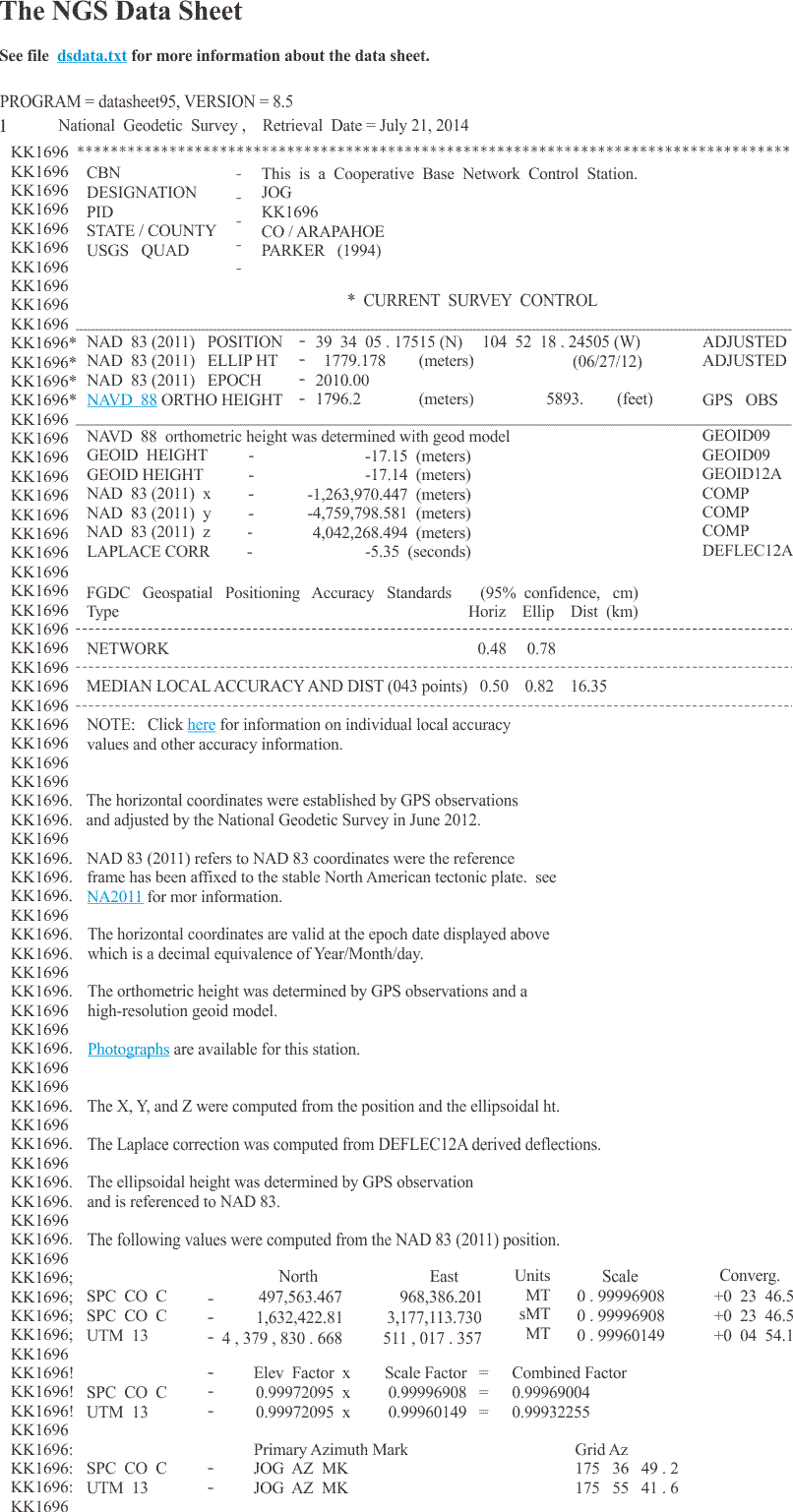
One of the things that is very useful is understanding the existing control that is currently available. Brass tablets and brass caps have been set around the United States by the National Geodetic Survey also known as passive marks. You can retrieve sheets that are similar to what you see in the illustration. These sheets have a great deal of excellent information concerning the coordinates, the quality, and many of the details about existing control points that can be used as checkpoints in any GPS/GNSS survey. Monuments that are the physical manifestation of the National Spatial Reference System (NSRS) and can be occupied with survey equipment are known as passive marks. They can provide reliable control when properly utilized. That utilization should be informed by an understanding of the datasheet that accompanies each station and is easily available online. There is a good deal of information about the passive survey monuments on each individual sheet. In addition to the latitude and longitude, the published data include the state plane coordinates in the appropriate zones. The first line of each data sheet includes the retrieval date. Then the station’s category is indicated. There are several, and among them are Continuously Operating Reference Station, Federal Base Network Control Station, and Cooperative Base Network Control Station. This is followed by the station’s designation, which is its name, and its Point Identification, PID. Either of these may be used to search for the station in the NGS database. The PID is also found all along the left side of each data sheet record and is always two upper case letters followed by four numbers. The state, county, country and U.S. Geological Survey (USGS)-7.5 minute quad name follows. Even though the station is located in the area covered by the quad sheet, it may not actually appear in the map. Under the heading, “Current Survey Control,” you will find the latitude and longitude of the station in NAD83 which is fixed to the North American plate, currently in NAD83 (2011), and its height in NAVD88. The orthometric height in meters is listed as “ORTHO HEIGHT” and followed by the same in feet. When the height is derived from GPS/GNSS observation, a geoid model must be used to determine the orthometric height. The model used is given. Adjustments to NAD27 and NGVD29 datums are a thing of the past. However, these old values may be shown under Superseded Survey Control. Horizontal values may be either Scaled, if the station is a benchmark or Adjusted, if the station is indeed a horizontal control point.
When a date is shown in parentheses after NAD83 in the data sheet, it means that the position has been readjusted. There are 13 sources of vertical control values shown on NGS data sheets. Here are a few of the categories. There is Adjusted, which are given to 3 decimal places and are derived from least squares adjustment of precise leveling. Another category is Posted, which indicates that the station was adjusted after the general NAVD adjustment in 1991. When a station’s elevation has been found by precise leveling but non-rigorous adjustment, it is called Computed. Stations’ vertical values are given to 1 decimal place if they are from GPS/GNSS observation (Obs) or vertical angle measurements (Vert Ang). And they have no decimal places if they were scaled from topographic map, Scaled, or found by conversion from NGVD29 values using the program known as VERTCON. The NGS Data Sheet.
When they are available, earth-centered earth-fixed (ECEF) coordinates are shown in X,Y and Z. These are right-handed system, 3-D Cartesian coordinates and are computed from the position and the ellipsoidal height. They are the same type of X, Y, and Z coordinates presented earlier. These values are followed by the quantity which, when added to an astronomic azimuth, yields a geodetic azimuth, is known as the Laplace correction. It is important to note that NGS uses a clockwise rotation regarding the Laplace correction. The ellipsoid height per the NAD83 ellipsoid is shown followed by the geoid height where the position is covered by NGS’s GEOID program. Photographs of the station may also be available in some cases. When the data sheet is retrieved online, one can use the link provided to bring them up. Also, the geoidal model used is noted. Of course, the first retrieval date at the top of the sheet is valuable to know when the point was last recovered. There's much detail here. I leave it to you to read. But suffice it to say for the objective here, the NGS data sheet is helpful to learn what control is available in a particular area.
Coordinates
NGS data sheets also provide State Plane and Universal Transverse Mercator (UTM) coordinates, the latter only for horizontal control stations. State Plane Coordinates are given in both U.S. Survey Feet or International Feet, and UTM coordinates are given in meters. Azimuths to the primary azimuth mark are clockwise from north and scale factors for conversion from ellipsoidal distances to grid distances. This information may be followed by distances to reference objects. Coordinates are not given for azimuth marks or reference objects on the data sheet.
The Station Mark
Along with mark setting information, the type of monument and the history of mark recovery, the NGS data sheets provide a valuable to-reach description. It begins with the general location of the station. Then starting at a well-known location, the route is described with right and left turns, directions, road names, and the distance traveled along each leg in kilometers. When the mark is reached, the monument is described, and horizontal and vertical ties are shown. Finally, there may be notes about obstructions to GPS/GNSS visibility, and so forth.
Significance of the Information
The value of the description of the monument’s location and the route used to reach it is directly proportional to the date it was prepared and the remoteness of its location. The conditions around older stations often change dramatically when the area has become accessible to the public. If the age and location of a station increases the probability that it has been disturbed or destroyed, then reference monuments can be noted as alternatives worthy of on-site investigation. However, special care ought to be taken to ensure that the reference monuments are not confused with the station marks themselves.
The role of passive marks is undergoing a change as a new North American reference frame takes shape (North American Terrestrial Reference Frame: NATRF). NGS is no longer setting nor maintaining passive marks.
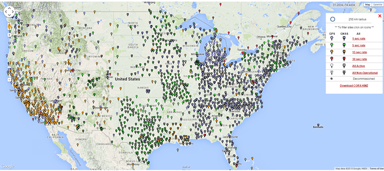
Control from Continuously Operating Networks
The requirement to occupy physical geodetic monuments in the field can be obviated by downloading the tracking data available online from appropriate continuously operating reference stations (CORS) where their density is sufficient. These stations, also known as Active Stations, comprise fiducial networks that support a variety of GPS/GNSS applications. While they are frequently administered by governmental organizations, some are managed by public-private organizations and some are commercial ventures. The most straightforward benefit of CORS is the user’s ability to do relative positioning without operating his own base station, by depending on that role being fulfilled by the network’s reference stations. While CORS can be configured to support differential GPS (DGPS) and real-time kinematic (RTK) applications, as in Real-Time Networks, most networks constantly collect GPS/GNSS tracking data from known positions and archive the observations for subsequent download by users from the Internet.
These days it is quite possible to not have to occupy an existing brass tablet, brass cap, such as indicated on this NGS data sheet. The reason for this is because of the continuously operating reference stations that have been established by the National Geodetic Survey are very useful. These active stations are a network and the most straightforward benefit is that a user can do relative positioning without operating his own base station and by depending on the CORS station, which as you see in this illustration downloads its reference information from tracking the GPS/GNSS network to an archived base station that is available on the Internet. You can access this and then combine it with the GPS/GNSS data that you have collected and post process for a differential, position a relative position, without having to occupy an existing control point on the ground.
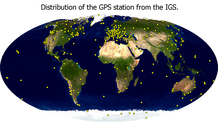
In many instances the original impetus of a network of CORS was geodynamic monitoring as illustrated by the GEONET established by the Geographical Survey Institute, GSI, in Japan after the Kobe earthquake. Networks that support the monitoring of the International Terrestrial Reference System, ITRS have been created around the world by the International GNSS Service, IGS, which is a service of the International Association of Geodesy and the Federation of Astronomical and Geophysical Data Analysis Services originally established in 1993. The United States is by no means the only place in which such networks exist.
Here is an illustration of the Southern California Integrated GPS/GNSS Network, SCIGN is a network run by a government-university partnership. More and more of these networks are appearing across the United States, sometimes on a statewide basis, county basis, and other regional designations. These continuously operating stations occupy a known position and then track the full constellation of GPS/GNSS satellites continuously. Then this data is made available, sometimes with a subscription cost, but in the case of NGS for free, and it is available then to do differential positioning of static GPS/GNSS sessions.
More on Continuously Operating Reference Station Networks
NGS Continuously Operating Reference Stations
The NGS CORS network is illustrated here. It includes hundreds of stations constantly logging GPS/GNSS data. The establishment of a CORS network, the result, has been a boon for high-accuracy GPS/GNSS positioning. Surveyors in the United States can take advantage of the CORS network administered by the National Geodetic Survey, NGS. The continental NGS system has two components, the Cooperative CORS and the National CORS. NGS manages the national CORS to support this post-processing for both code and carrier phase observations. The Cooperative CORS system supplements the National CORS system. The NGS does not directly provide the data from the cooperative system of stations. Its stations are managed by participating university, public, and private organizations that operate the sites. These cooperative arrangements mean that we all can use the data free on charge in most cases. That data can then be conveniently downloaded in its original form from the Internet free of charge for up to 30 days after its collection. It is also available later, but after it has been decimated to a 30-second format. The data is available in the Receiver Independent Exchange Format, or RINEX format. The RINEX format allows you to use any type of a receiver to log your data because this RINEX format is available from virtually every kind of standard GPS/GNSS receiver.
Nearly all coordinates provided by NGS for the CORS sites are available in NAD83 (2011) epoch 2010.0. The coordinates of CORS stations are also published in ITRF2014 (2010.0). These positions differ from NAD83(2011). All the coordinates are accompanied by velocities since the stations are moving. These velocities can be used to calculate the stations position at a different date using NGS’s Horizontal Time Dependent Positioning (HTDP) utility.
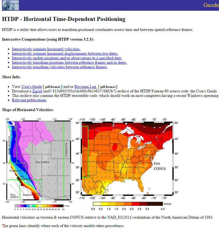
Here (above) is an illustration of the Horizontal Time-Dependent Positioning website.
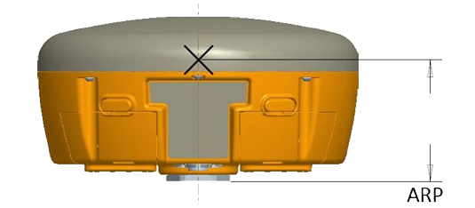
At a CORS site, NGS provides the coordinates of the L1 phase center and the Antenna Reference Point (ARP). Generally speaking, it is best to adopt the position that can be physically measured, that means the coordinates given for the ARP. It is the coordinate of the part of the antenna from which the phase center offsets are calculated that is usually the bottom mount. The phase centers of antennas are not immovable points. They actually change slightly, mostly as the elevation of the satellite’s signals change. In any case, the phase centers for L1, L2 and L5 differ from the position of the ARP both vertically and horizontally. NGS provides the position of the phase center on average at a particular CORS site. As most postprocessing software will, given the ARP, provide the correction for the phase center of an antenna, based on antenna type, the ARP is the most convenient coordinate value to use. The distance to the ARP is often given from the bottom of the mount, as indicated by this diagram.
International GNSS Service (IGS)
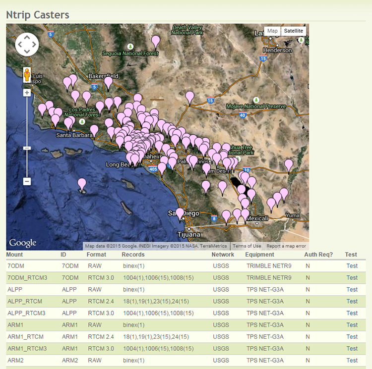
Like NGS, IGS also provides CORS data. However, it has a global scope. The information on the individual stations can be accessed, including the ITRF Cartesian coordinates and velocities for the IGS sites, but not all the sites are available from IGS servers. The Scripps Orbit and Permanent Array Center (SOPAC) is a convenient access point for IGS data. A virtual map of the available GPS/GNSS networks can be found there.
Tracking data is from international networks. Here you see a graphic of its extent. It's virtually worldwide. You can download the tracking information from these antennas, these known positions, to post-process the data from a roving GPS/GNSS antenna internationally.
The Scripps Orbit and Permanent Array Center
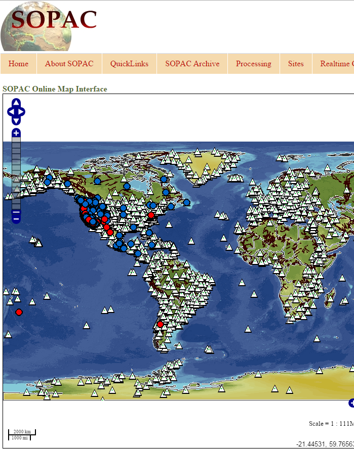
SOPAC is a convenient access point for IGS data.
Static Survey Project Design
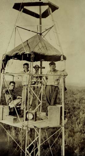
Image ID: 1618, NOAA's Historic Coast & Geodetic Survey (C&GS) Collection
Location: Ozark Mountains, Missouri
Photo Date: 1935
Source: http://www.photolib.noaa.gov/cgs/triangulation.html
Publication of the US Dept. of Commerce, NOAA, NOAA Central Library, COAA Privacy Policy / NOAA Desclaimer
Last Updated: April 23, 2007
Static Survey Project Design
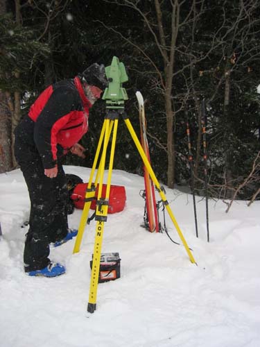
The selection of satellites to track, start and stop times, mask elevation angle, assignment of data file names, reference position, bandwidth, and sampling rate are some options useful in the static mode, as other GPS/GNSS surveying methods. These features may appear to be prosaic, but their practicality is not always obvious. For example, satellite selection can seem unnecessary when using a receiver with sufficient independent channels to track all satellites above the receiver’s horizon without difficulty. However, a good survey project design pays dividends by limiting lost time and maximizing productivity. When geodetic surveying was more dependent on optics than electronic signals from space, horizontal control stations were set with station intervisibility in mind, not ease of access. Therefore, it is not surprising that stations established in that way are frequently difficult to reach. Not only are they found on the tops of buildings and mountains, they are also in woods, beside transmission towers, near fences, and generally obstructed from GPS/GNSS signals. The geodetic surveyors that established them could hardly have foreseen a time when a clear view of the sky above their heads would be crucial to high-quality control. The illustration shows some surveyors on a Bilby tower, high above the Ozark Mountains in Missouri. Their observations were done at night with angles turned to far away lights to establish horizontal control by triangulation. It's hardly surprising that at the time surveyors were working on these towers they weren't terribly concerned with the sky visibility at the stations they occupied and set. They were concerned with getting high enough over obstructions to see the other stations.
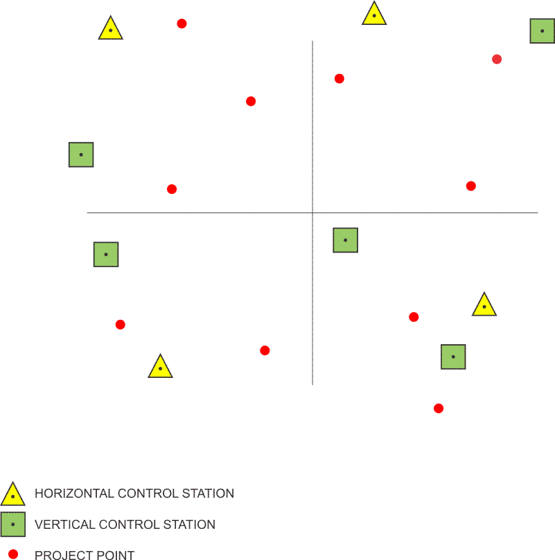
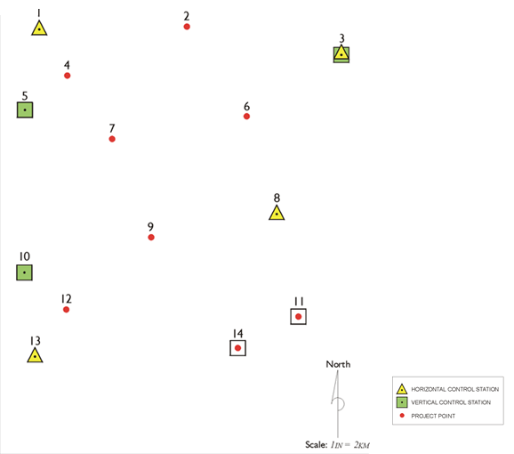
In fact, it is only recently that most private surveyors have had any routine use for NGS stations. Many station marks have not been occupied for quite a long time. Since the primary monuments are often found deteriorated, overgrown, unstable, or destroyed. The role of passive marks is changing rapidly. In any case, it is a good idea to propose reconnaissance of several more than the absolute minimum of three horizontal control stations. Fewer than three makes any check of their positions virtually impossible. Many more are usually required in a GPS/GNSS route survey. In general, in GPS/GNSS networks, the more -chosen horizontal control stations that are available, the better. Some stations will almost certainly prove unsuitable unless they have been used previously in GPS/GNSS work. The location of the stations, relative to the GPS/GNSS project itself, is also an important consideration in choosing horizontal control. For work other than route surveys, a handy rule of thumb is to divide the project into four quadrants and to choose at least one horizontal control station in each. The actual survey should have at least one horizontal control station in three of the four quadrants. Each of them ought to be as near as possible to the project boundary. Supplementary control in the interior of the network can then be used to add more stability to the network. At a minimum, route surveys require horizontal control at the beginning, the end, and the middle. Long routes should be bridged with control on both sides of the line at appropriate intervals. The standard symbol for indicating horizontal control on the project map is a triangle.
Vertical Control
Those stations with a published accuracy high enough for consideration as vertical control are symbolized by an open square or circle on the map. Those stations that are sufficient for horizontal control are symbolized as triangles. Where there is horizontal and vertical control the symbol is a combination of the triangle and square.
A minimum of four vertical control stations are needed to anchor a GPS/GNSS static network. A large project should have more. In general, the more benchmarks available the better. Vertical control is best located at the four corners of a project. Orthometric elevations are best transferred by means of classic spirit leveling; such work should be built into the project plan when it is necessary. When spirit levels are planned to provide vertical control positions, special care may be necessary to ensure that the precision of such conventional work is as consistent as possible with the rest of the survey. Route surveys require vertical control at the beginning and the end. They should be bridged with benchmarks on both sides of the line at intervals from 5 to 10 km. When the distances involved are too long for spirit leveling to be used effectively, two independent GPS/GNSS measurements may suffice to connect a benchmark to the project. However, it is important to recall the difference between the ellipsoidal heights available from a GPS/GNSS observation and the orthometric elevations yielded by a level circuit.
Plotting Project Points
A solid dot is the standard symbol used to indicate the position of project points. Some variation is used when a distinction must be drawn between those points that are in place and those that must be set.
When its location is appropriate, it is always a good idea to have a vertical or horizontal control station serve double duty as a project point. While the precision of their plotting may vary, it is important that project points be located as precisely as possible even at this preliminary stage. The subsequent observation schedule will depend to some degree on the arrangement of the baselines. Also, the preliminary evaluation of access, obstructions, and other information depends on the position of the project point relative to these features. In the design, the project points are indicated. These are the points on which coordinates are going to be required based upon the control available around them.
Evaluating Access
When all potential control and project positions have been plotted and given a unique identifier, some aspects of the survey can be addressed a bit more specifically. If good roads are favorably located, if open areas are indicated around the stations, and if no station falls in an area where special permission will be required for its occupation, then the preliminary plan of the survey ought to be remarkably trouble-free. However, it is likely that one or more of these conditions will not be so fortunately arranged. The speed and efficiency of transportation from station to station can be assessed to some degree from the project map. It is also wise to remember that while inclement weather does not disturb GPS/GNSS observations whatsoever, without sufficient preparation it can play havoc with surveyors’ ability to reach points over difficult roads or by aircraft. Since in a static GPS/GNSS survey, the control points and the points to be coordinated—the project points—need to be occupied simultaneously, they need to observe the same constellation of satellites at the same time. It's important to be able to be on the station ready to observe when the sessions begin, simultaneously on control and project points.
Planning Offsets
If control stations or project points are located in areas where the map indicates that topography or vegetation will obstruct the satellite’s signals, alternatives may be considered. A shift of the position of a project point into a clear area may be possible where the change does not have a significant effect on the overall network. A control station may also be the basis for a less obstructed position, transferred with a short level circuit or traverse. Of course, such a transfer requires availability of conventional surveying equipment on the project. In situations where such movement is not possible, careful consideration of the actual paths of the satellites at the station itself during on-site reconnaissance may reveal enough windows in the gaps between obstructions to collect sufficient data by strictly defining the observation sessions.
Planning Azimuth Marks
Azimuth marks are a common requirement in GPS/GNSS projects. They are an accompaniment to static GPS/GNSS stations when a client intends to use them to control subsequent conventional surveying work. Of course, the line between the station and the azimuth mark should be as long as convenience and the preservation of line-of-sight allows. It is wise to take care that short baselines do not degrade the overall integrity of the project. Occupations of the station and its azimuth mark should be simultaneous for a direct measurement of the baseline between them. Both should also be tied to the larger network as independent stations. There should be two or more occupations of each station when the distance between them is less than 2 km. An alternative approach may be to derive the azimuth between a GPS/GNSS station and its azimuth mark with an astronomic observation.

Obtaining Permissions
Another aspect of access can be considered when the project map finally shows all the pertinent points. Nothing can bring a well-planned survey to a halt faster than a locked gate, an irate landowner, or a government official that is convinced he should have been consulted previously. To the extent that it is possible from the available mapping, affected private landowners and government jurisdictions should be identified and contacted. Taking this precaution at the earliest stage of the survey planning can increase the chance that the sometimes long process of obtaining permissions, gate keys, badges, or other credentials has a better chance of completion before the survey begins.
Any aspect of a GPS/GNSS survey plan derived from examining mapping, virtual or hardcopy, must be considered preliminarily. Most features change with time, and even those that are relatively constant cannot be portrayed on a map with complete exactitude. Nevertheless, steps toward a coherent workable design can be taken using the information they provide.
Control Project Design Facts
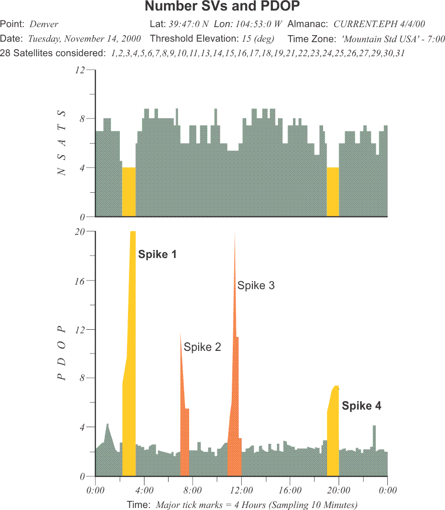
Though much of the preliminary work in producing the plan of a GPS/GNSS survey is a matter of estimation, some hard facts must be considered, too. For example, the number of GPS/GNSS receivers available for the work and the number of satellites above the observer’s horizon at a given time in a given place are two ingredients that can be determined with some certainty. Most GPS/GNSS software packages provide users with routines that help them determine the satellite windows, the periods of time when the largest numbers of satellites are simultaneously available. Today, observers are virtually assured of 24-hour coverage; however, the mere presence of adequate satellites above an observer’s horizon does not guarantee collection of sufficient data. Therefore, despite the virtual certainty that at least 4 satellites will be available, evaluation of their configuration as expressed in the position dilution of precision (PDOP) is still crucial in planning a GPS/GNSS survey. Satellites need to be available for observation at the occupied points. The same satellites need to be visible at both ends of the vectors that are going to be occupied. Most GPS/GNSS software packages allow you to know how many satellites are above a horizon at a particular location. The position dilution of precision (PDOP) is also something that needs to be taken into account in a static GPS/GNSS survey design. Here are some charts that indicate how PDOP can be evaluated in some cases. You see here the number of satellites on the left. On the right, you see the position dilution of precision. It spikes when the number of satellites drops, when some set. When there are only four, the PDOP goes way up. The geometry of the satellites from the receiver's point of view is not optimal. There are some other spikes, too, as the satellites move from one configuration to another. It is not wise to do GPS/GNSS observations when the PDOP is high. You need to be aware of those times so that in planning the observation schedule, you’re not trying to measure baselines when the PDOP is spiking.
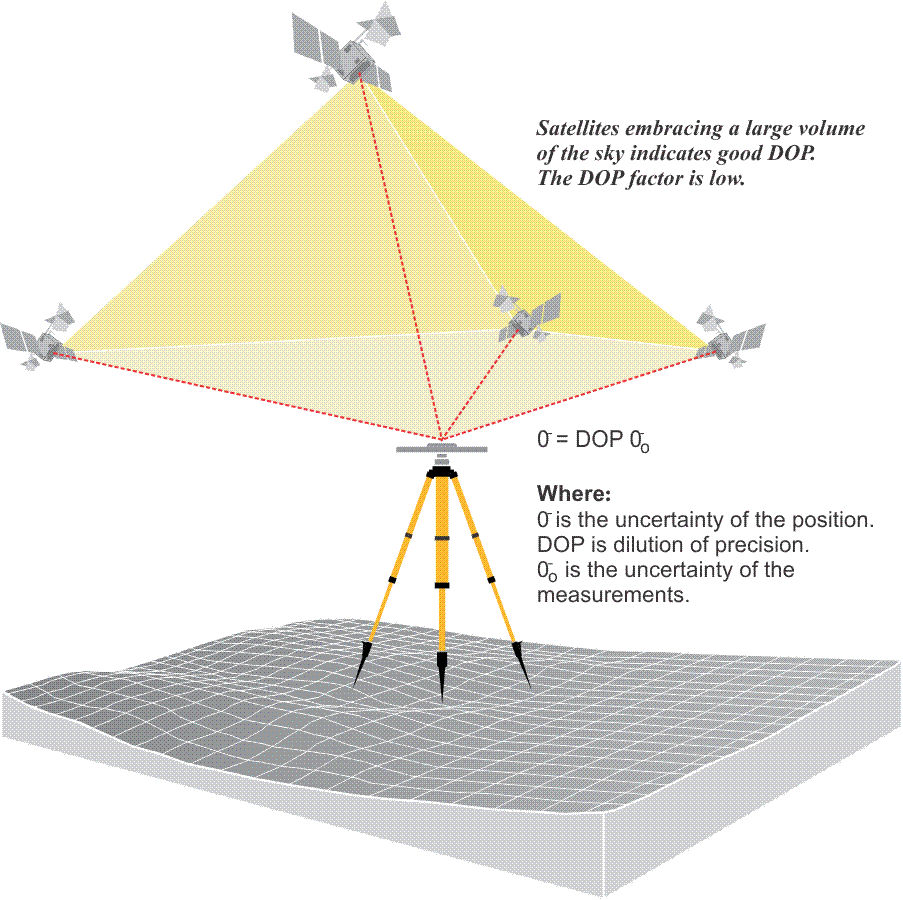
Position Dilution of Precision (PDOP)
The assessment of the productivity of a GPS/GNSS survey almost always hinges, in part at least, on the length of the observation sessions required to satisfy the survey specifications. The determination of the session’s duration depends on several particulars, such as the length of the baseline and the relative position, that is the geometry, of the satellites, among others. Generally speaking, the larger the constellation of satellites, the better the available geometry, the lower the positioning dilution of precision (PDOP), and the shorter the length of the session needed to achieve the required accuracy. For example, given 6 satellites and good geometry, baselines of 10 km or less might require a session of 45 minutes to 1 hour, whereas, under exactly the same conditions, a baseline over 20 km might require a session of 2 hours or more. Alternatively, 45 minutes of 6-satellite data may be worth an hour of 4-satellite data, depending on the arrangement of the satellites in the sky. Stated another way, the GPS/GNSS receiver’s position is derived from the simultaneous solution of vectors between it and the constellation of satellites above the observer’s horizon. The quality of that solution depends, in large part, on the distribution of those vectors. For example, any position determined when the satellites are crowded together in one part of the sky will be unreliable, because all the vectors will have virtually the same direction. Fortunately, a computer can predict such an unfavorable configuration if it is given the ephemeris of each satellite, the approximate position of the receiver, and the time of the planned observation. Provided with a forecast of a large PDOP, the GPS/GNSS survey planner should consider an alternate observation plan. On the other hand, when one satellite is directly above the receiver and three others are near the horizon (but not too close) and 120° in azimuth from one another, the arrangement is nearly ideal for a 4-satellite constellation. The planner of the survey would be likely to consider such a window. However, more satellites would improve the resulting position even more, as long as they are well distributed in the sky above the receiver. In general, the more satellites, the better. For example, if the planner finds 8 satellites will be above the horizon in the region where the work is to be done and the PDOP is below 2, that window would be a likely candidate for observation. There are other important considerations. The satellites are constantly moving in relation to the receiver and to each other. Because satellites rise and set, the PDOP is constantly changing. Within all this movement, the GPS/GNSS survey designer must have some way of correlating the longest and most important baselines with the longest windows, the most satellites, and the lowest PDOP. Most GPS/GNSS software packages, given a particular location and period of time, can provide illustrations of the satellite configuration.
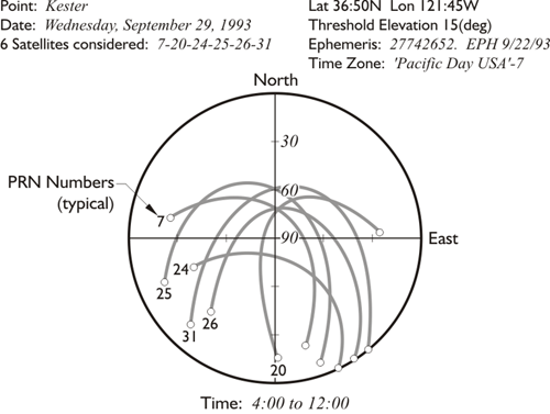
Polar Plot
One such diagram is a plot of the satellite’s tracks drawn on a graphical representation of the upper half of the celestial sphere with the observer’s zenith at the center and perimeter circle as the horizon. The azimuths and elevations of the satellites above the specified 15-degree mask angle are connected into arcs that represent the paths of all available satellites. The utility of this sort of drawing has lessened with the completion of the GPS/GNSS constellation. In fact, there are so many satellites available that the picture can become quite crowded and difficult to decipher.
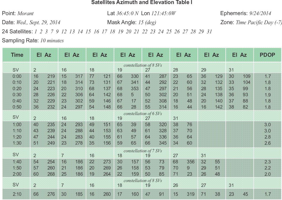
An example: the position of point Morant in the table needed expression to the nearest minute only, a sufficient approximation for the purpose. The ephemeris data were 5 days old when the chart was generated by the computer, but the data were still an adequate representation of the satellite’s movements to use in planning. The mask angle was specified at 15°, so the program would consider a satellite set when it moved below that elevation angle. The zone time was Pacific Daylight Time, 7 hours behind Coordinated Universal Time, UTC. The full constellation provided 24 healthy satellites, and the sampling rate indicated that the azimuth and elevation of those above the mask angle would be shown every 10 minutes. This is all in view. You could use this to plan particular observation windows when four or more satellites were up, the PDOP over there on the far right was at an acceptable level. These all seem to be fairly good. And then, one can plan the periods that you'll be observing from particular stations.
At 0:00 hour, satellite PRN 2 could be found on an azimuth of 219° and an elevation of 16° above the horizon by an observer at 36°45'Nf and 121°45'W?. The table indicates that PRN 2 was rising, and got continually higher in the sky for the 2 hours and 10 minutes covered by the chart. The satellite PRN 16 was also rising at 0:00, but reached its maximum altitude at about 1:10 and began to set. Unlike PRN 2, PRN 16 was not tabulated in the same row throughout the chart. It was supplanted when PRN 7 rose above the mask angle and PRN 16 shifted one column to the right. The same may be said of PRN 18 and PRN 19. Both of these satellites began high in the sky, unlike PRN 28 and PRN 29. They were just above 15° and setting when the table began and set after approximately 1 hour of availability. They would not have been seen again at this location for about 12 hours. This chart indicated changes in the available constellation from eight space vehicles, SVs, between 0:00 and 0:50, six between 1:00 and 1:30, seven from 1:40 to 2:00 and back to eight at 2:10. The constellation never dipped below the minimum of four satellites, and the PDOP was good throughout. The PDOP varied between a low of 1.7 and a high of 3.0. Over the interval covered by the table, the PDOP never reached the unsatisfactory level of 5 or 6, which is when a planner should avoid observation.
Choosing the Window
Using this chart, the GPS/GNSS survey designer might well have concluded that the best available window was the first. There was nearly an hour of 8-satellite data with a PDOP below 2. However, the data indicated that good observations could be made at any time covered here, except for one thing: it was the middle of the night.
Ionospheric Delay
It is worth noting that the ionospheric error is usually smaller after sundown. In fact, the FGDC specified dual-frequency receivers for daylight observations for the achievement of the highest accuracies, due, in part, to the increased ionospheric delay during those hours. When planning the survey, it's always useful to note that the ionospheric error is smaller after sundown. The table above shows data from later in the day. It covers a period of two hours when a constellation of 5 and 6 satellites was always available. However, through the first hour, from 6:30 to 7:30, the PDOP hovered around 5 and 6. For the first half of that hour, four of the satellites—PRN 9, PRN 12, PRN 13, and PRN 24—were all near the same elevation. During the same period, PRN 9 and PRN 12 were only approximately 50° apart in azimuth, as well. Even though a sufficient constellation of satellites was constantly available, the survey designer may well have considered only the last 30 to 50 minutes of the time covered by this chart as suitable for observation. There is one caution, however. Azimuth-elevation tables are a convenient tool in the division of the observing day into sessions, but it should not be taken for granted that every satellite listed is healthy and in service. For the actual availability of satellites and an update on atmospheric conditions, it is always wise to check. In the planning stage, the diligence can prevent creation of a design dependent on satellites that prove unavailable. Similarly, after the field work is completed, it can prevent inclusion of unhealthy data in the postprocessing.
Supposing that the period from 7:40 to 8:30 was found to be a good window, the planner may have regarded it as a single 50-minute session, or divided it into shorter sessions. One aspect of that decision was probably the length of the baseline in question. In static GPS/GNSS, a long line of 30 km may require 50 minutes of 6-satellite data, but a short line of 3 km may not. Another consideration was probably the approximation of the time necessary to move from one station to another.
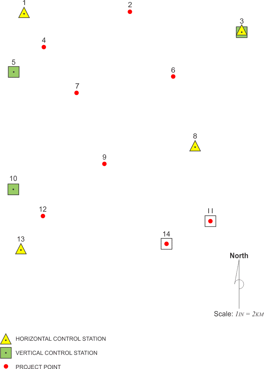
Drawing the Baselines
Horizontal Control
A good rule of thumb is to verify the integrity of the horizontal control by observing baselines between these stations first. The vectors can be used to both corroborate the accuracy of the published coordinates and later to resolve the scale, shift, and rotation parameters between the control positions and the new network that will be determined by GPS/GNSS. These baselines are frequently the longest in the project, and there is an added benefit to measuring them first. By processing a portion of the data collected on the longest baselines early in the project, the most appropriate length of the subsequent sessions can be found. This test may allow improvement in the productivity on the job without erosion of the final positions. By observing the horizontal control baselines first, you can discover any difficulty with the published coordinates. For example, if they are NGS brass caps, you would learn if there is any discrepancy with the published coordinates on these control stations.
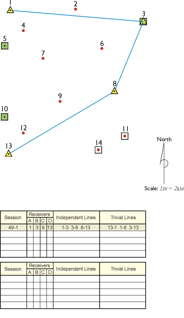
Julian Day in Naming Sessions
The table in the illustration indicates that the name of the first session connecting the horizontal control is 49-1. The date of the planned session is given in the Julian system. Taken most literally, Julian dates are counted from January 1, 4713 B.C. However, most practitioners of GPS/GNSS use the term to mean the day of the current year measured consecutively from January 1. Under this construction, since there are 31 days in January, Julian day 49 is February 18. The designation 49-1 means that this is to be the first session on that day. Some prefer to use letters to distinguish the session. In that case, the label would be 49-A.
Independent Lines
This project will be done with four receivers. The table shows that receiver A will occupy point 1; receiver B, point 3; receiver C, point 8; and receiver D, point 13 in the first session. Where r is the number of receivers, every session yields r-1 independent baselines. That is why the illustration shows only three of the possible six base lines that will be produced by this arrangement. Only the independent, also known as nontrivial, lines are shown on the map. The three lines that are not drawn are called trivial, and are also known as dependent lines. This idea is based on restricting the use of the lines created in each observing session to the absolute minimum needed to produce a unique solution. In the planning stage, it is best to consider the shortest vectors independent and the three longest lines are eliminated as trivial, or dependent. That is the case with the session illustrated but it cannot be said that the shortest lines are always chosen to be the independent lines. Sometimes, there are reasons to reject one of the shorter vectors due to incomplete data, cycle slips, multipath, or some other weakness in the measurements. Before such decisions can be made, each session will require analysis after the data has actually been collected.
Another aspect of the distinction between independent and trivial lines involves the concept of error of closure, or loop closure. Loop closure is a procedure by which the internal consistency of a GPS/GNSS network is discovered. A series of baseline vector components from more than one GPS/GNSS session, forming a loop or closed figure, is added together. The closure error is the ratio of the length of the line representing the combined errors of all the vector’s components to the length of the perimeter of the figure. Any loop closures that only use baselines derived from a single common GPS/GNSS session will yield an apparent closure error of zero, because they are derived from the same simultaneous observations. For example, all the baselines between the four receivers in session 49-1 of the illustrated project will be based on ranges to the same GPS/GNSS satellites over the same period of time. Therefore, the trivial lines of 13- 1, 1-8, and 3-13 will be derived from the same information used to determine the independent lines of 1-3, 3-8, and 8-13. It follows that, if the fourth line from station 13 to station 1 were included to close the figure of the illustrated session, the error of closure would be zero. The same may be said of the inclusion of any of the trivial lines. Their addition cannot add any redundancy or any geometric strength to the lines of the session, because they are all derived from the same data. If redundancy cannot be added to a GPS/GNSS session by including any more than the minimum number of independent lines, how can the baselines be checked? Where does redundancy in GPS/GNSS work come from?
Redundancy
Redundancy means stations being measured more than once. It is a useful thing in trying to evaluate the accuracy or the correctness of a network.
If only two receivers were used to complete the illustrated project, there would be no trivial lines and it might seem there would be no redundancy at all. But to connect every station with its closest neighbor, each station would have to be occupied at least twice, and each time during a different session. For example, with receiver A on station 1 and receiver B on station 2, the first session could establish the baseline between them. The second session could then be used to measure the baseline between station 1 and station 4. It would certainly be possible to simply move receiver B to station 4 and leave receiver A undisturbed on station 1. However, some redundancy could be added to the work if receiver A were reset. If it were re-centered, re-plumbed, and its H.I. (height of instrument) re-measured, some check on both of its occupations on station 1 would be possible when the network was completed. Under this scheme, a loop closure at the end of the project would have some meaning. If one were to use such a scheme on the illustrated project and connect into one loop all of the 14 baselines determined by the 14 two-receiver sessions, the resulting error of closure would be useful. It could be used to detect blunders in the work, such as mis-measured H.I.s. Such a loop would include many different sessions. The ranges between the satellites and the receivers defining the baselines in such a circuit would be from different constellations at different times. On the other hand, if it were possible to occupy all 14 stations in the illustrated project with 14 different receivers simultaneously and do the entire survey in one session, a loop closure would be absolutely meaningless.
As soon as three or more receivers are considered, the discussion of redundant measurement must be restricted to independent baselines, excluding trivial lines. In the real world, such a project is not done with 14 receivers nor with 2 receivers, but with 3, 4, or 5. The achievement of redundancy takes a middle road. Redundancy is then defined by the number of independent baselines that are measured more than once, as well as by the percentage of stations that are occupied more than once. While it is not possible to repeat a baseline without reoccupying its endpoints, it is possible to reoccupy a large percentage of the stations in a project without repeating a single baseline. These two aspects of redundancy in GPS/GNSS - the repetition of independent baselines and the reoccupation of stations - are somewhat separate.
The illustration above shows one of the many possible approaches to setting up the baselines for this particular GPS/GNSS project. The design in the illustration shows lines in different colors showing the occupations using four GPS/GNSS receivers and how they are used through simultaneous occupation on these stations to create a network. The session numbers are in the table, the independent and trivial lines are listed. The A, B, C, and D receivers are shown and what points they occupy, at what stages. This is obviously done over 10 sessions over two consecutive days, and there's a good deal of redundancy in the network. However, that's simply the design. That doesn't mean that that's what will actually occur.
The survey design calls for the horizontal control to be occupied in session 49-1. It is to be followed by measurements between two control stations and the nearest adjacent project points in session 49-2. As shown in the table at the bottom of the figure, there will be redundant occupations on stations 1 and 3. Even though the same receivers will occupy those points, their operators will be instructed to reset them at a different H.I.s for the new session. A better, but probably less efficient, plan would be to occupy these stations with different receivers than were used in the first session.
Forming Loops
As the baselines are drawn on the project map for a static GPS/GNSS survey, or any GPS/GNSS work where accuracy is the primary consideration, the designer should remember that part of their effectiveness depends on the formation of complete geometric figures. When the project is completed, these independent vectors should be capable of formation into closed loops that incorporate baselines from two to four different sessions. In the illustrated baseline plan, no loop contains more than ten vectors, no loop in more than 100 km long, and every observed baseline will have a place in a closed loop.
Ties to the Vertical Control
The ties from the vertical control stations to the overall network are usually not handled by the same methods used with the horizontal control. The first session of the illustrated project was devoted to occupation of all the horizontal control stations. There is no similar method with the vertical control stations. First, the geoidal undulation would be indistinguishable from baseline measurement error. Second, the primary objective in vertical control is for each station to be adequately tied to its closest neighbor in the network. If a benchmark can serve as a project point, it is nearly always advisable to use it, as was done with stations 11 and 14 in the illustrated project. A conventional level circuit can often be used to transfer a reliable orthometric elevation from vertical control station to a nearby project point.
Finding the Number of Sessions
where
s = the number of observing sessions,
r = the number of receivers,
m = the total number of stations involved
Finding the Number of Sessions
The illustrated survey design calls for 10 sessions, but the calculation does not include human error, equipment breakdown, and other unforeseeable difficulties. It would be impractical to presume a completely trouble-free project. The FGCC proposed the following formula for arriving at a more realistic estimate. But n, p, and k require a bit more explanation. The variable n is a representation of the level of redundancy that has been built into the network, based on the number of occupations on each station. The illustrated survey design includes more than two occupations on all but 4 of the 14 stations in the network. In fact, 10 of the 14 positions will be visited three or four times in the course of the survey. There are a total of 40 occupations by the 4 receivers in the 10 planned sessions. By dividing 40 occupations by 14 stations, it can be found that each station will be visited an average of 2.857 times. Therefore, the planned redundancy represented by factor n is equal to 2.857 in this project.
The experience of a firm is symbolized by the variable p in the formula. The division of the final number of actual sessions required to complete past projects by the initial estimation yields a ratio that can be used to improve future predictions. That ratio is the production factor, p. A typical production factor is 1.1. A safety factor of 0.1, known as k, is recommended for GPS projects within 100 km of a company’s home base. Beyond that radius, an increase to 0.2 is advised.
The substitution of the appropriate quantities for the illustrated project increases the prediction of the number of observation sessions required for its completion:
In other words, the 2-day, 10-session schedule is a minimum period for the baseline plan drawn on the project map. A more realistic estimate of the observation schedule includes 14 sessions. It is also important to keep in mind that the observation schedule does not include time for on-site reconnaissance.
Static GPS/GNSS Control Surveying
The prospects for the success of a GPS/GNSS project are directly proportional to the quality and training of the people doing it. The handling of the equipment, the on-site reconnaissance, the creation of field logs, and the inevitable last-minute adjustments to the survey design all depend on the training of the personnel involved for their success. There are those who say the operation of GPS/GNSS receivers no longer requires highly qualified survey personnel. That might be true if effective GPS/GNSS surveying needed only the pushing of the appropriate buttons at the appropriate time. In fact, when all goes as planned, it may appear to the uninitiated that GPS/GNSS has made experienced field surveyors obsolete. But when the unavoidable breakdowns in planning or equipment occur, the capable people, who seemed so superfluous moments before, suddenly become indispensable. Also, the full range of conventional surveying equipment and expertise have a place in GPS/GNSS. For some, their role may be more abbreviated than it was formerly, but one element that can never be outdated is good judgment.
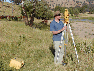
Conventional Equipment
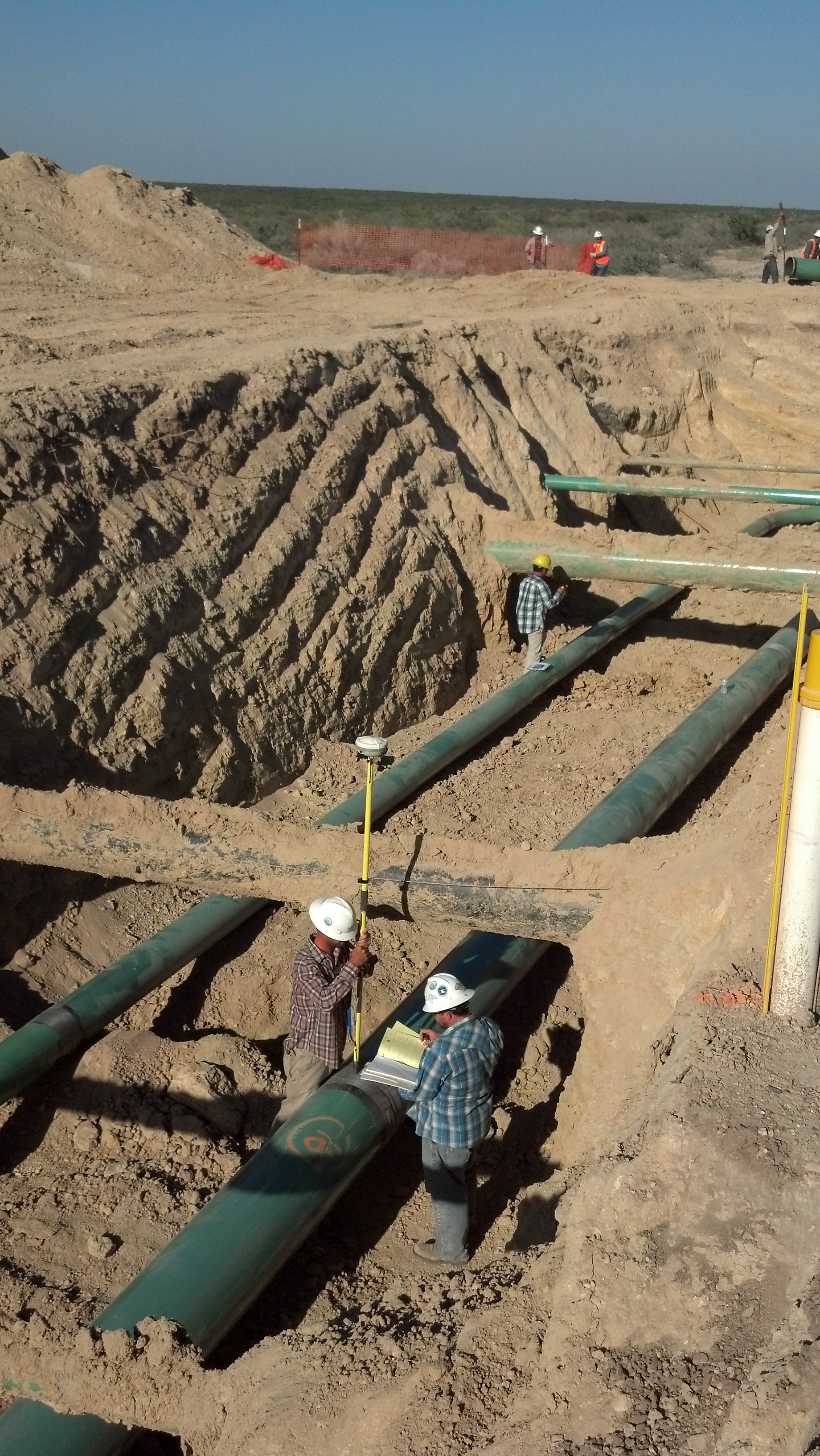
Most GPS/GNSS projects require conventional surveying equipment for spirit-leveling circuits, offsetting horizontal control stations, and monumenting project points, among other things. It is perhaps a bit ironic that this most advanced surveying method also frequently has the need of the most basic equipment. The use of brush hooks, machetes, axes, and so forth, can sometimes salvage an otherwise unusable position by removing overhead obstacles. Another strategy for overcoming such hindrances has been developed, using various types of survey masts to elevate a separate GPS/GNSS antenna above the obstructing canopy. Flagging, paint, and the various techniques of marking that surveyors have developed over the years are still a necessity in GPS/GNSS work. The pressure of working in unfamiliar terrain is often combined with urgency. Even though there is usually not a moment to spare in moving from station to station, a GPS/GNSS surveyor frequently does not have the benefit of having visited the particular points before. In such situations, the clear marking of both the route and the station during reconnaissance is vital. Despite the best route marking, a surveyor may not be able to reach the planned station, or, having arrived, finds some new obstacle or unanticipated problem that can only be solved by marking and occupying an impromptu offset position for a session. A hammer, nails, shiners, paint, and so forth are essential in such situations.
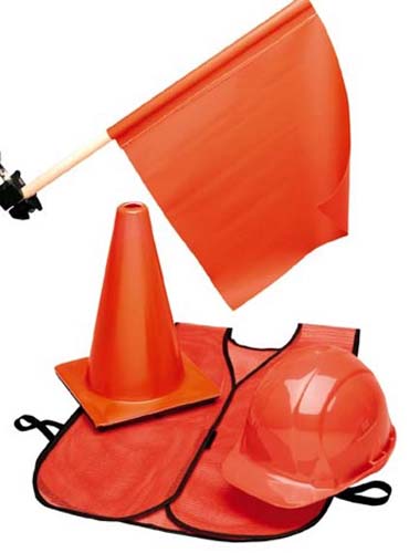
Safety equipment
The high-visibility vests, cones, lights, flagmen, and signs needed for traffic control cannot be neglected in GPS/GNSS work. Unlike conventional surveying operations, GPS/GNSS observations are not deterred by harsh weather. Occupying a control station in a highway is dangerous enough under the best of conditions, but in the midst of a rainstorm, fog, or blizzard, it can be absolute folly without the proper precautions. And any time and trouble taken to avoid infraction of the local regulations regarding traffic management will be compensated by an uninterrupted observation schedule.
Communications
Whether the equipment is handheld or vehicle mounted, two-way radios and cell phones are used in most GPS/GNSS operations. However, the line of sight that is no longer necessary for the surveying measurements in GPS/GNSS is sorely missed in the effort to maintain clear radio contact between the receiver operators. A radio link between surveyors can increase the efficiency and safety of a GPS/GNSS project, but it is particularly valuable when last-minute changes in the observation schedule are necessary. When an observer is unable to reach a station, or a receiver suddenly becomes inoperable, unless adjustments to the schedule can be made quickly, each end of all of the lines into the missed station will require reobservation. The success of static GPS/GNSS hinges on all receivers collecting their data simultaneously. However, it is more and more difficult to ensure reliable communication between receiver operators in geodetic surveys, especially as their lines grow longer. High-wattage, private-line FM radios are quite useful when line of sight is available between them or when a repeater is available. The use of cell phones may eliminate the communication problem in some areas, but probably not in remote locations. Despite the limitations of the systems available at the moment, achievement of the best possible communication between surveyors on a GPS/GNSS project pays dividends in the long run.
Information
The information every GPS/GNSS observer carries throughout a project ought to include emergency phone numbers; the names, addresses, and phone numbers of relevant property owners; and the combinations to necessary locks. Each member of the team should also have a copy of the project map, any other maps that are needed to clarify position or access, and, perhaps most important of all, the updated observation schedule. The observation schedule for static GPS/GNSS work will be revised daily based upon actual production. It should specify the start–stop times and station for all the personnel during each session of the upcoming day. In this way, the schedule will not only serve to inform every receiver operator of his or her own expected occupations, but those of every other member of the project as well. This knowledge is most useful when a sudden revision requires observers to meet or replace one another.
| Svs PRNs | Session 1 Start 7:10 Stop 8:10 9, 12, 13, 16, 20, 24 |
8:10 to 8:40 |
Session 2 Start 8:40 Stop 9:50 3, 12, 13, 16, 20, 24 |
9:50 to 10:15 |
Session 3 Start 10:15 Stop 11:15 3, 12, 13, 16, 17, 20, 24 |
11:15 to 11:30 |
Session 4 Start 11:30 Stop 12:30 3, 16, 17, 20, 22, 23, 26 |
12:30 to 14:00 |
Session 5 Start 14:00 Stop 15:00 1, 3, 17, 21, 23, 26, 28 |
|---|---|---|---|---|---|---|---|---|---|
| Receiver A Dan H. |
Station 1 NGS Horiz. Control |
Re-Set | Station 1 NGS Horiz. Control |
Move | Station 5 NGS Benchmark |
Re-Set | Station 5 NGS Benchmark |
Re-Set | Station 5 NGS Benchmark |
| Receiver B Scott G. |
Station 3 NGS V&H Control |
Re-Set | Station 3 NGS V&H Control |
Move | Station 6 Project Point |
Re-Set | Station 6 Project Point |
Move | Station 1 NGS Horiz. Control |
| Receiver C Dewey A. |
Station 8 NGS Horiz. Control |
Move | Station 2 Project Point |
Re-Set | Station 2 Project Point |
Move | Station 7 Project Point |
Move | Station 10 NGS Benchmark |
| Receiver D Cindy E. |
Station 13 NGS Horiz. Control |
Move | Station 4 Project Point |
Re-Set | Station 4 Project Point |
Move | Station 9 Project Point |
Move | Station 13 NGS Horiz. Control |
This page shows an observation schedule for a static control survey. And as you see here, the sessions are numbered as to when they start and when they stop. And then the receiver A, B, C, and D is shown and what station they are to be on and what they are to do when they move from one to another. This sort of log is necessary when static surveying is done. Because, of course, the constellation needs to be observed simultaneously with GPS/GNSS receivers occupying the points here.
For example, receiver A on Station One, receiver B on Station Three, C on eight, and D on 13 and Session One need to be at that position beginning at 7:10 and stopping at 8:10 so that we will have a full hour of simultaneous observations on those stations. Then some reset and stay at the same place, and others move on to another station. For example, one and three reset, and Station 8 and 13 move. Station 8 moves to Station 2, Station 13 moves to Station 4. And then, of course, there's a half an hour given there for that move. And at 8:40, they all power up and observe till 9:50. This gives you an idea of how it is necessary to have the information of this well in hand when one does the work. This observation schedule can be revised, of course, if the observations don't go as planned. It should specify start and stop times. In this way, the schedule will not only serve to inform every receiver operator of his or her own expected occupations, but those of every other in the project as well. This is useful, sometimes, when unexpected occurrences cause a change in the schedule.
Station Data
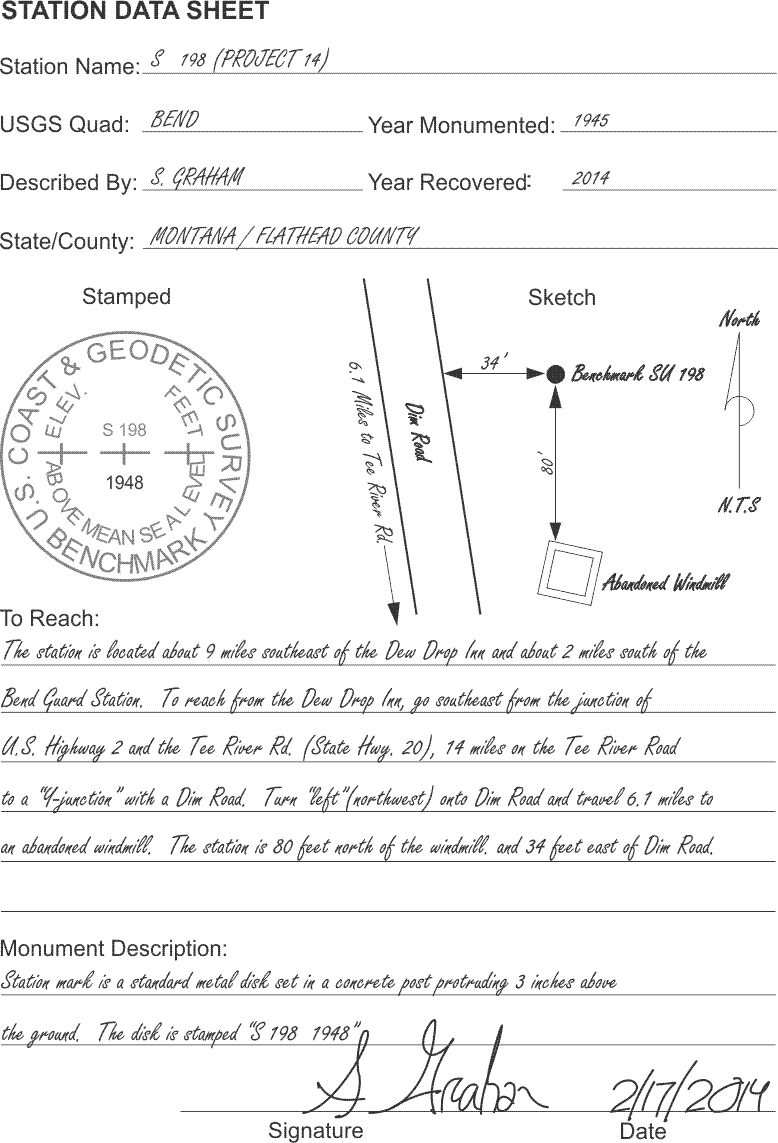
Station Data Sheet
Click here to see a text description.
Station Data Sheet
Station Name: S 198 (Project 14)
USGS Quad: BEND
Year Monumented: 1945
Described by: S GRAHAM
Year Recovered: 2014
State/County: MONTANA/FLATHEAD COUNTY
stamp and sketch included
To Reach: The station is located about 9 miles southeast of the Dew Drop Inn and about 2 miles south of the Bend Guard Station. To reach from the Dew Drop Inn, go southeast from the junction of US Highway 2 and the Tee River Rd. (State Hwy. 20), 14 miles on the Tee River Road to a "4-Junction" with a Dim Road. Turn "left" (northwest) onto Dim Road and travel 6.1 miles to an abandoned windmill. The station is 80 feet north of the windmill, and 34 feet east of Dim Road.
Monument Description: Station mark is a standard metal disk set in a concrete post protruding three inches above the ground. The disk is stamped "S 198 1948"
Signature: S. Graham
Date: 2/17/14
The principles of good field notes have a long tradition in land surveying, and they will continue to have validity for some time to come. In GPS/GNSS, the ensuing paper trail will not only fill subsequent archives; it has immediate utility. For example, the station data sheet is often an important bridge between on-site reconnaissance and the actual occupation of a monument. Though every organization develops its own unique system of handling its field records, most have some form of the station data sheet. The document illustrated here is merely one possible arrangement of the information needed to recover the station. The station data sheet can be prepared at any period of the project, but perhaps the most usual times are during the reconnaissance of existing control or immediately after the monumentation of a new project point. Neatness and clarity, always paramount virtues of good field notes, are of particular interest when the station data sheet is to be later included in the final report to the client. The overriding principle in drafting a station data sheet is to guide succeeding visitors to the station without ambiguity. A GPS/GNSS surveyor on the way to observe the position for the first time may be the initial user of a station data sheet. A poorly written document could void an entire session if the observer is unable to locate the monument. A client, later struggling to find a particular monument with an inadequate data sheet, may ultimately question the value of more than the field notes.
Here is an example of a station data sheet. This is the sort of information that will be recorded again in a static control survey to show the station that has been occupied, show a sketch of where it is located relative to other fixed landmarks, and then other information—how to reach it, a description of the monument, and of course, a signature and a date.
Station name
The station name fills the first blank on the illustrated data sheet. Two names for a single monument is far from unusual. In this case the vertical control station, officially named S 198, is also serving as a project point, number 14. But two names purporting to represent the same position can present a difficulty. For example, when a horizontal control station is remonumented, a number 2 is sometimes added to the original name of the station, and it can be confusing. For example, it can be easy to mistake a station, "Thornton 2," with an original station named, "Thornton," that no longer exists. Both stations may still have a place in the published record, but with slightly different coordinates. Another unfortunate misunderstanding can occur when inexperienced field personnel mistake a reference mark, R.M., for the actual station itself. The taking of rubbings and/or close-up photographs are widely recommended to avoid such blunders regarding stations names or authority.
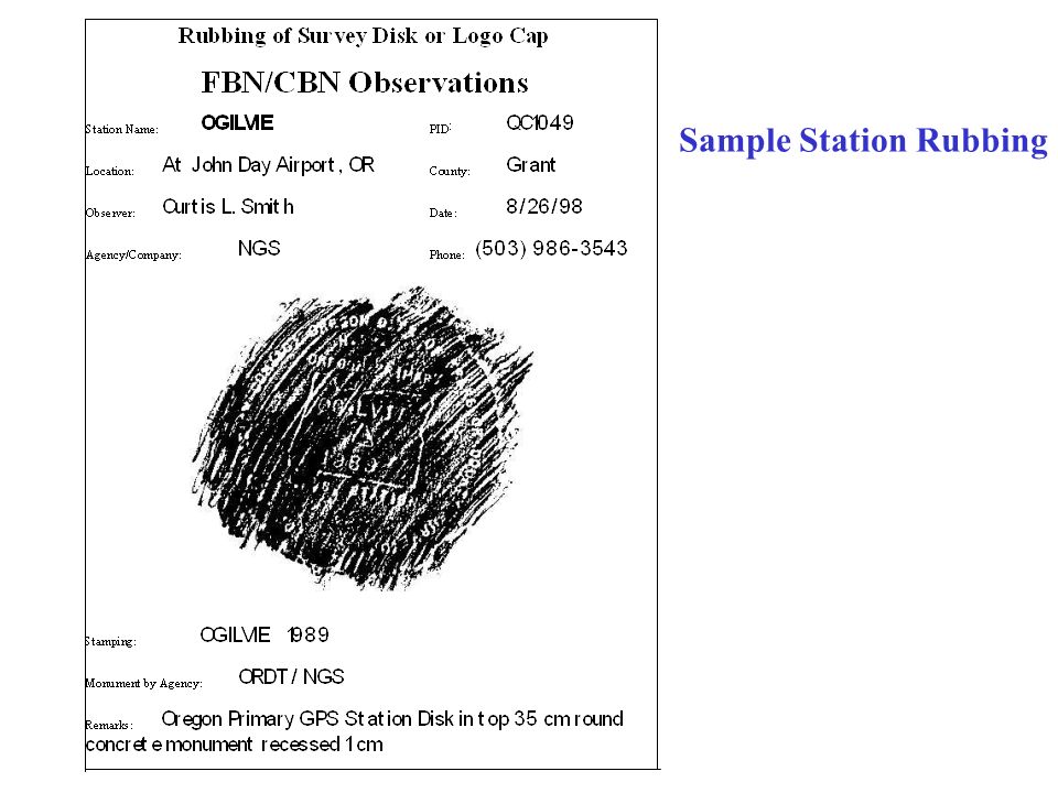
Station Rubbing
Source: https://slideplayer.com/slide/9394640/
Rubbings
The illustrated station data sheet provides an area to accommodate a rubbing. With the paper held on top of the monument’s disk, a pencil is run over it in a zigzag pattern, producing a positive image of the stamping. This method is a bit more awkward than simply copying the information from the disk onto the data sheet, but it does have the advantage of ensuring the station was actually visited and that the stamping was faithfully recorded. Such rubbings or close-up photographs are often required.
Photographs
The use of photographs is growing as a help for the perpetuation of monuments. It can be convenient to photograph the area around the mark as well as the monument itself. These exposures can be correlated with a sketch of the area. Such a sketch can show the spot where the photographer stood and the directions toward which the pictures were taken. The photographs can then provide valuable information in locating monuments, even if they are later obscured. Still, the traditional ties to prominent features in the area around the mark are the primary agent of their recovery. It's important to have an idea of exactly what the monument looked like and to ensure that the intended point was occupied.
Quad Sheet Name
Providing the name of the appropriate state, county, and USGS quad sheet helps to correlate the station data sheet with the project map. The year the mark was monumented, the monument description, the station name, and the "to-reach" description all help to associate the information with the correct official control data sheet and, most importantly, the correct station coordinates.
To-reach descriptions
When driving or walking to a position can be aided by computerized turn-by-turn navigation, it is a great tool that may make writing to-reach descriptions unnecessary. However, GPS/GNSS control work is often done in areas where the roadway mapping in such navigation aids is inadequate. In those situations, the description of the route to the station is one of the most critical documents written during the reconnaissance. Even though it is difficult to prepare the information in unfamiliar territory and although every situation is somewhat different, there are some guidelines to be followed. It is best to begin with the general location of the station with respect to easily found local features. The description in the top illustration relies on a road junction, a guard station, and a local business. After defining the general location of the monument, the description should recount directions for reaching the station. Starting from a prominent location, the directions should adequately describe the roads and junctions. Where the route is difficult or confusing, the reconnaissance team should not only describe the junctions and turns needed to reach a station; it is wise to also mark them with lath and flagging, when possible. It is also a good idea to note gates. Even if they are open during reconnaissance, they may be locked later. When turns are called for, it is best to describe not only the direction of the turn, but the direction of the new course too. For example, in the description in the station data sheet at the top, the turn onto the dim road from the Tee River Road is described to the,"left (northwest)." Roads and highways should carry both local names and designations found on standard highway maps. For example, in the illustrated form, Tee River Road is also described as State Highway 20. The "to-reach" description should certainly state the mileages, as well as the travel times where they are appropriate, particularly where packing-in is required. Land ownership, especially if the owner's consent is required for access, should be mentioned. The reconnaissance party should obtain the permission to enter private property and should inform the GPS/GNSS observer of any conditions of that entry. Alternate routes should be described where they may become necessary. It is also best to make special mention of any route that is likely to be difficult in inclement weather. Where helicopter access is anticipated, information about the duration of flights from point to point, the distance of landing sites from the station, and flight time to fuel supplies should be included on the station data sheet.
Flagging and Describing the Monument
Flagging the station during reconnaissance may help the observer find the mark more quickly. On the station data sheet, the detailed description of the location of the station with respect to roads, fence lines, buildings, trees, and any other conspicuous features should include measured distances and directions. A clear description of the monument itself is important. It is wise to also show and describe any nearby marks, such as reference monuments (R.M.'s) that may be mistaken for the station or aid in its recovery. The name of the preparer, a signature, and the date round out the initial documentation of a GPS/GNSS station.
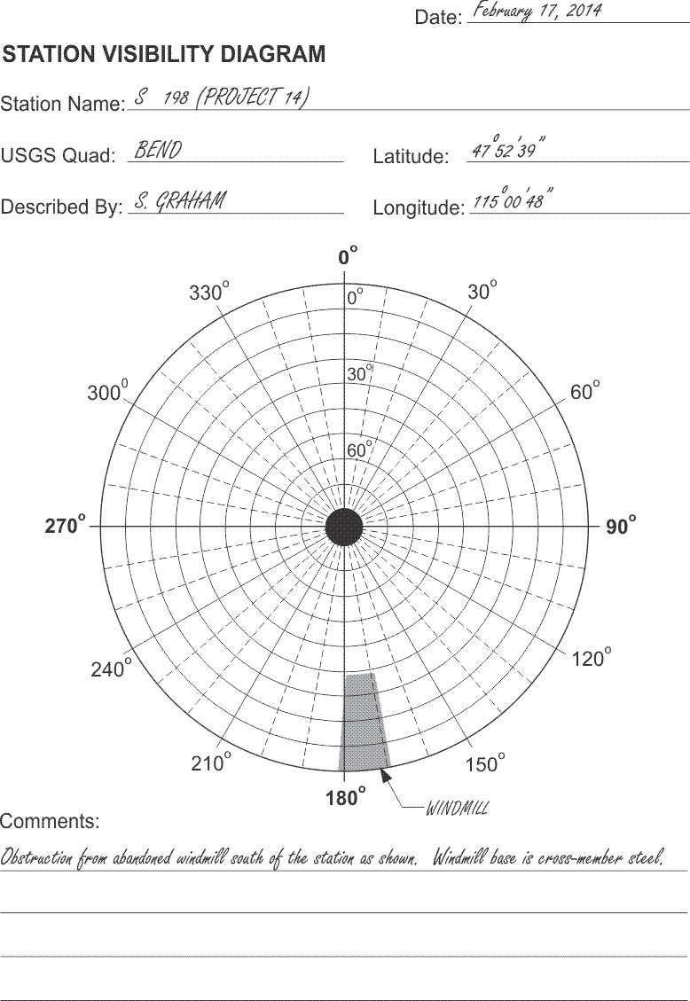
Visibility Diagram and Satellites Azimuth/Elevation Tables
Click here to see a text description.
Station Visibility Diagram
Date: February 17, 2014
Station Name: S 198 (PROJECT 14)
Described By: S. GRAHAM
USGS Quad: BEND
Latitude: 47 degrees 52'39"
Longitude: 115 degrees 00'48"
radial diagram showing where the windmill is located
Comments: Obstruction from abandoned windmill south of the station as shown. Windmill base is cross-member steel.
Obstructions above the mask angle of a GPS/GNSS receiver must be taken into account in finalizing the observation schedule. A station that is blocked to some degree is not necessarily unusable, but its inclusion in any particular session is probably contingent on the position of the specific satellites involved.
It is important for GPS/GNSS observations to have a good view of the sky. Obstructions above the mask angle must be taken into account, especially with static control survey.
An Example
The diagram in the illustration is widely used to record such obstructions during reconnaissance. It is known as a station visibility diagram, a polar plot, or a skyplot. The concentric circles are meant to indicate 10° increments along the upper half of the celestial sphere, from the observer’s horizon at 0° on the perimeter, to the observer’s zenith at 90° in the center. The hemisphere is cut by the observer’s meridian, shown as a line from 0° in the north to 180° in the south. The prime vertical is signified as the line from 90° in the east to 270° in the west. The other numbers and solid lines radiating from the center, every 30° around the perimeter of the figure, are azimuths from north and are augmented by dashed lines every 10°.
Drawing obstructions
Using a compass and a clinometer, a member of the reconnaissance team can fully describe possible obstructions of the satellite’s signals on a visibility diagram. By standing at the station mark and measuring the azimuth and vertical angle of points outlining the obstruction, the observer can plot the object on the visibility diagram. For example, a windmill base is shown on in the illustration as a cross-hatched figure. It has been drawn from the observer's horizon up to 37° in vertical angle, from 168° to about 182° in azimuth at its widest point. This description by approximate angular values is entirely adequate for determining when particular satellites may be blocked at this station.
Once completed, this diagram allows you to correlate the obstructions shown with other charts that give you the number of satellites available, the azimuth and height of those satellites at a particular time. With all this information, you will be able to design the observation session on this particular point so that satellites will not be obstructed.
| Time | SV 3 Elev. |
SV 3 Azim. |
SV 12 Elev. |
SV 12 Azim. |
SV 13 Elev. |
SV 13 Azim. |
SV 20 Elev. |
SV 20 Azim. |
SV 24 Elev. |
SV 24 Azim. |
Elev. |
Azim. |
PDOP |
|---|---|---|---|---|---|---|---|---|---|---|---|---|---|
| 8:50 | 54 | 235 | 74 | 274 | 44 | 28 | 16 | 308 | 68 | 169 | 4.8 | ||
| 9:00 | 51 | 229 | 74 | 255 | 40 | 32 | 20 | 310 | 72 | 163 | 5.7 | ||
| 9:10 | 47 | 224 | 72 | 238 | 37 | 35 | 23 | 311 | 77 | 153 | 4.9 | ||
| 9:20 | 43 | 219 | 68 | 226 | 33 | 38 | 27 | 313 | 80 | 134 | 1.0 |
| Time | SV 3 Elev. |
SV 3 Azim. |
SV 12 Elev. |
SV 12 Azim. |
SV& 13 Elev. |
SV 13 Azim. |
SV 16 Elev. |
SV 16 Azim. |
SV 20 Elev. |
SV 20 Azim. |
SV 24 Elev. |
SV 24 Azim. |
PDOP |
|---|---|---|---|---|---|---|---|---|---|---|---|---|---|
| 9:30 | 39 | 215 | 64 | 218 | 29 | 41 | 16 | 179 | 31 | 314 | 81 | 102 | 2.1 |
| 9:40 | 35 | 212 | 59 | 213 | 26 | 45 | 19 | 176 | 36 | 314 | 80 | 73 | 2.3 |
| 9:50 | 31 | 209 | 54 | 209 | 23 | 48 | 23 | 173 | 40 | 315 | 76 | 57 | 2.4 |
| 10:00 | 27 | 207 | 49 | 206 | 19 | 52 | 27 | 170 | 44 | 314 | 72 | 49 | 2.5 |
| 10:10 | 23 | 204 | 44 | 204 | 16 | 55 | 30 | 167 | 48 | 314 | 67 | 45 | 2.5 |
For example, suppose a 1-hour session from 9:10 to 10:10, illustrated in this table, was under consideration for the observation on station S 198. The station visibility chart might motivate a careful look at space vehicle (SV) pseudorandom noise (PRN) 16. Twenty minutes into the anticipated session, at 9:30 SV 16 has just risen above the 15° mask angle. Under normal circumstances, it would be available at station S 198, but it appears from the polar plot that the windmill will block its signals from reaching the receiver. In fact, the signals from SV 16 will apparently not reach station S 198 until sometime after the end of the session at 10:10.
Working around Obstructions
Under the circumstances, some consideration might be given to observing station S 198 during a session when none of the satellites would be blocked. However, the 9:10 to 10:10 session may be adequate after all. Even if SV 16 is completely blocked, the remaining 5 satellites will be unobstructed, and the constellation still will have a relatively low position dilution of precision (PDOP). Still, the analysis must be carried to other stations that will be occupied during the same session. The success of the measurement of any baseline depends on common observations at both ends of the line. Therefore, if the signals from SV 16 are garbled or blocked from station S 198, any information collected during the same session from that satellite at the other end of a line that includes S 198 will be useless in processing the vector between those two stations.
However, the material of the base of the abandoned windmill has been described on the visibility diagram as cross-membered steel, so it is possible that the signal from SV 16 will not be entirely obstructed during the whole session. There may actually be more concern of multipath interference from the structure than that of signal availability. One strategy for handling the situation might be to program the receiver at S 198 to ignore the signal from SV 16 completely if the particular receiver allows it. The visibility diagram and the azimuth-elevation table complement each other. They provide the field supervisor with the data needed to make informed judgments about the observation schedule. Even if the decision is taken to include station S 198 in the 9:10 to 10:10 session as originally planned, the supervisor will be forewarned that the blockage of SV 16 may introduce a bit of weakness at that particular station.
Multipath

The multipath condition is by no means unique to GPS/GNSS. When a transmitted television signal reaches the receiving antenna by two or more paths, the resulting variations in amplitude and phase cause the picture to have ghosts. This kind of scattering of the signals can be caused by reflection from land, water, or man-made structures. In GPS/GNSS, the problem can be particularly troublesome when signals are received from satellites at low elevation angles; hence, the general use of a 15° to 20° mask angle. The use of choke ring antennas to mediate multipath may also be considered. It is also wise, where it is possible, to avoid using stations that are near structures likely to be reflective or to scatter the signal. For example, chain-link fences that are found hard against a mark can cause multipath by forcing the satellite’s signal to pass through the mesh to reach the antenna. The elevation of the antenna over the top of the fence with a survey mast is often the best way to work around this kind of obstruction. Metal structures with large flat surfaces are notorious for causing multipath problems. A long train moving near a project point could be a potential problem, but vehicles passing by on a highway or street usually are not, especially if they go by at high speed. It is important, of course, to avoid parked vehicles. It is best to remind new GPS/GNSS observers that the survey vehicle should be parked far enough from the point to avert any multipath. A good way to handle these unfavorable conditions is to set an offset point.
Avoiding obstructions is a significant part of planning and performing a good GPS/GNSS observation.
Point Offsets
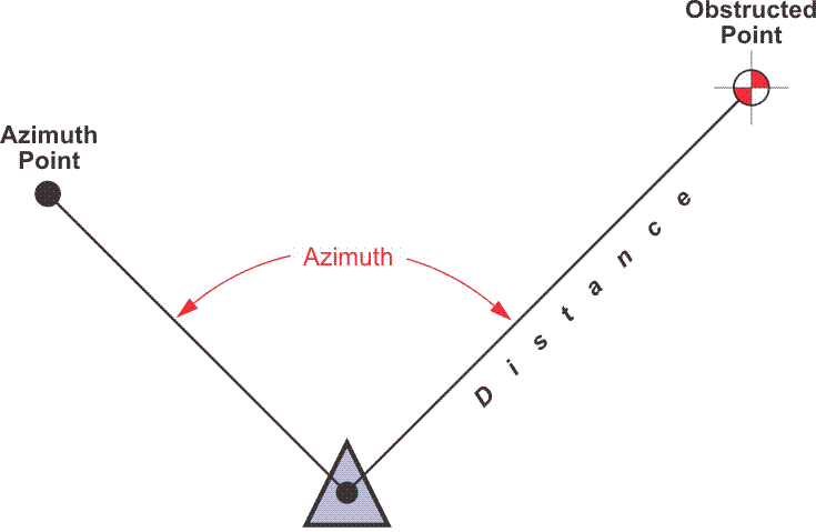
An offset must, of course, stand far enough away from the source of multipath or an attenuated signal to be unaffected. However, the longer the distance from the originally desired position, the more important the accuracy of the bearing and distance between that position and the offset becomes. Recording the tie between the two correctly is crucial to avoid misunderstanding after the work is completed. Some receivers allow input of the information directly into the observations recorded in the receiver or data logger. However, during a control survey, it is best to also record the information in a field book. Offsets in GPS/GNSS control surveying are an instance where conventional surveying equipment and expertise are necessary. Clearly, the establishment of the tie requires a position for the occupation of the instrument, i.e. a total station, and a position for the establishment of its orientation, that is, an azimuth. It is best to establish three intervisible rather than two points—one to occupy and two azimuth marks. This approach makes it possible to add a redundant check to the tie. The positions of these two, or three, points may be established by setting monuments and performing static observations on them all. Alternatively, azimuthal control may be established by astronomic observations.
Monumentation
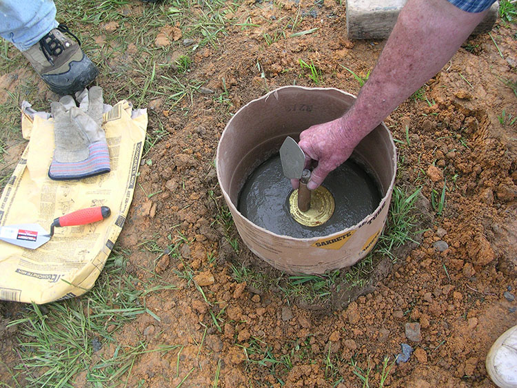
The monumentation set for GPS/GNSS projects varies widely and can range from brass tablets to aerial premarks, capped rebar or even pin flags. The objective of most station markers is to adequately serve the client's subsequent use. However, the time, trouble, and cost in most high-accuracy GPS/GNSS work warrants the most permanent, stable monumentation. Many experts predict that GPS/GNSS will eventually make monumentation unnecessary. The idea foresees GPS/GNSS receivers in constant operation at well-known master (i.e. CORS) stations will allow surveyors with receivers to determine highly accurate relative positions with such speed and ease that monumentation will be unnecessary. The idea may prove prophetic, but, for now, monumentation remains an important part of most GPS/GNSS projects. The suitability of a particular type of monument is an area still most often left to the professional judgement of the surveyors involved.
Observation
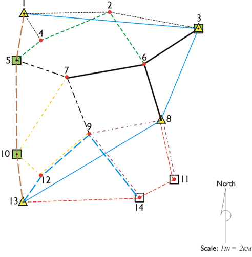
When everything goes as planned, a GPS/GNSS observation is uneventful. However, even before the arrival of the receiver operator at the control or project point, the session can get off-track. The simultaneity of the data collected at each end of a baseline is critical to the success of any measurement in static GPS/GNSS control surveys. When a receiver occupies a master station throughout a project, there need be little concern on this subject. But most static applications depend on the sessions of many mobile receivers beginning and ending together.
Arrival
The number of possible delays that may befall an observer on the way to a station are too numerous to mention. With proper planning and reconnaissance, the observer will likely find that there is enough time for the trip from station to station and that sufficient information is on hand to guide the observer to the position, but this, too, cannot be guaranteed. When the observer is late to the station, the best course is usually to set up the receiver quickly and collect as much data as possible. The baselines into the late station may or may not be saved, but they will certainly be lost if the receiver operator collects no information at all. It is at times like these that good communication between the members of the GPS/GNSS team is most useful. For example, some of the other observers in the session may be able to stay on their station a bit longer with the late arrival and make up some of the lost data. Along the same line, it is usually a good policy for those operators who are to remain on a station for two consecutive sessions to collect data as long as possible, while still leaving themselves enough time to reset between the two observation periods.
Set-up
Centering an instrument over the station mark is always important. However, the centimeter-level accuracy of static GPS/GNSS gives the centering of the antenna special significance. It is ironic that such a sophisticated system of surveying can be defeated from such a commonplace procedure. A tribrach with an optical plummet or any other device used for centering should be checked and, if necessary, adjusted before the project begins. With good centering and leveling procedures, an antenna should be within a few millimeters of the station mark. Unfortunately, the centering of the antenna over the station does not ensure that its phase center is properly oriented. The contours of equal phase around the antenna’s electronic center are not themselves perfectly spherical. Part of their eccentricity can be attributed to unavoidable inaccuracies in the manufacturing process. To compensate for some of this offset, it is a good practice to rotate all antennas in a session to the same direction. Many manufacturers provide reference marks on their antennas so that each one may be oriented to the same azimuth. That way, they are expected to maintain the same relative position between their physical and electronic centers when observations are made.
Height of Instrument
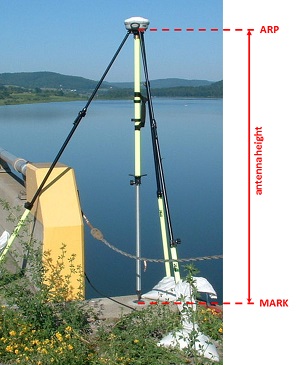
The care ascribed to the measurement of antenna heights is due to the same concern applied to centering. GPS/GNSS has an extraordinary capability to achieve accurate ellipsoidal heights, but those heights can be easily contaminated by incorrect H.I.s.
Most GPS/GNSS receivers capable of geodetic accuracy are designed to be mounted on a tripod, usually with a tribrach and adaptor. However, there is a trend toward bipod- or range-pole-mounted antennas. An advantage of these devices is that they ensure a constant height of the antenna above the station. The mismeasured height of the antenna above the mark is probably the most pervasive and frequent blunder in GPS/GNSS control surveying. The tape or rod used to measure the height of the antenna is sometimes built into the receiver and sometimes a separate device. It is important that the height of the instrument (H.I.) be measured accurately and consistently in both feet and meters, without merely converting from one to the other mathematically. It is also important that the value be recorded in the field notes and, where possible, also entered into the receiver itself. Since many systems measure the height of the antenna to the edge of the ground plane or to the exterior of the receiver itself, the calibration of the tribrach affects both the centering and the H.I. measurement. The resetting of a receiver that occupies the same station in consecutive sessions is an important source of redundancy for many kinds of GPS/GNSS networks. However, integrity can only be added if the tribrach has been accurately calibrated.
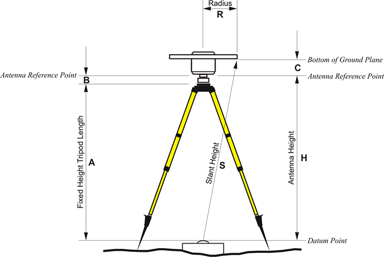
The measurement of the height of the antenna in a GPS/GNSS survey is often not made on a plumb line. A tape is frequently stretched from the top of the station monument to some reference mark on the antenna or the receiver itself. Some GPS/GNSS teams measure and record the height of the antenna to more than one reference mark on the ground plane. These measurements are usually mathematically corrected to plumb.
Observation Logs
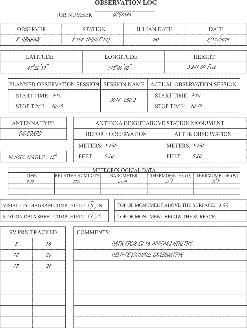
The most immediate use of the observation log is an evaluation of the day's work. Most GPS/GNSS control survey operations require its receiver operators to keep a careful log of each observation. Usually written on a standard form, these field notes provide a written record of the measurements, times, equipment, and other data that explains what actually occurred during the observation itself. It is difficult to overestimate the importance of this information. It is usually incorporated into the final report of the survey, the archives, and any subsequent effort to blue-book the project. However, the most immediate use of the observation log is in evaluation of the day's work by the on-site field supervisor. An observation log may be organized in a number of ways. The log illustrated is one method that includes some of the information that might be used to document one session at one station. Of course, the name of the observer and the station must be included, and while the date need not be expressed in both the Julian and Gregorian calendars, that information may help in quick cataloging of the data. The approximate latitude, longitude, and height of the station are usually required by the receiver as a reference position for its search for satellites. The date of the planned session will not necessarily coincide with the actual session observed. The observer's arrival at the point may have been late, or the receiver may have been allowed to collect data beyond the scheduled end of the session. There are various methods used to name the observation session in terminology that is sensible to computers. A widely used system is noted here. The first four digits are the project point’s number. In this case, it is point 14 and is designated 0014. The next three digits are the Julian day of the session, in this case it is day 50, or 050. Finally, the session illustrated is the second of the day, or 2. Therefore, the full session name is 0014 050 2. Whether onboard or separate, the type of the antenna used and the height of the antenna are critical pieces of information. The relation of the height of the station to the height of the antenna is vital to the station’s later utility. The distance that the top of the station's monument is found above or below the surface of the surrounding soil is sometimes neglected. This information can not only be useful in later recovery of the monument, but can also be important in the proper evaluation of photo-control panel points.
Weather
The meteorological data is useful in modeling the atmospheric delay. Measurement of the atmospheric pressure in millibars, the relative humidity, and the temperature in degrees Centigrade are sometimes expected to be in the observation log. However, the general use is less stringent. The conditions of the day are observed, and unusual changes in the weather are noted. A record of the satellites that are actually available during the observation and any comments about unique circumstances of the session round out the observation log.
Daily Progress Evaluation
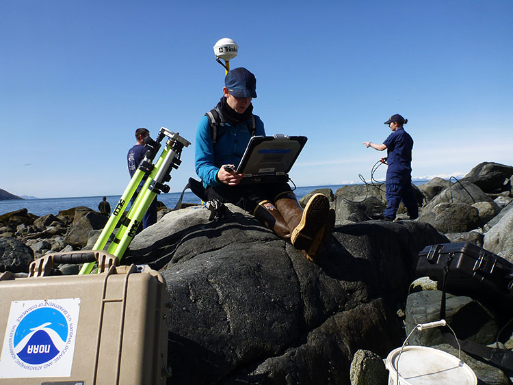
The planned observation schedules of a large GPS/GNSS project usually change daily. The arrangements of upcoming sessions are often altered based on the success or failure of the previous day’s plan. Such a regrouping follows an evaluation of the day’s data. This evaluation involves examination of the observation logs as well as the data each receiver has collected. Unhealthy data, caused by cycle slips or any other source, are not always apparent to the receiver operator at the time of the observation. Therefore, a daily quality control check is a necessary preliminary step before finalizing the next day’s observation schedule. Some field supervisors prefer to compute the independent baseline vectors of each day’s work to ensure that the measurements are adequate. Obviously, if a vector has failed, it's important to know it the very day it occurred so that it can be picked up in the subsequent day or days. Neglecting the daily check could leave unsuccessful sessions undiscovered until the survey was thought to be completed. The consequences of such a situation could be expensive.
Online Post-Processing Services
Using a Processing Service
An alternative to in-house post-processing is the use of a processing service. There are several services available to GPS/GNSS surveyors. While they differ somewhat in their requirements, they are all based on the same idea. Static GPS/GNSS data collected in the field may be uploaded to a website on the Internet by the hosting organization, which will then return the final positions, often free of charge. Usually, the user is directed to an ftp site where the results can be downloaded. There can be advantages to the use of such a processing service. Aside from removing the necessity of having post-processing software in-house, there is the strength of the network solution available from them. In other words, rather than the data sent in by the GPS/GNSS surveyor being processed against a single CORS in the vicinity of the work, it is processed against a group of the nearest CORS. There are often three in the group. Such a network-based solution improves the integrity of the final position markedly and may compensate for long baselines required by the sparseness of the CORS in the area of interest. Among the online resources available for processing services is the National Geodetic Survey's Online Positioning User Service (OPUS). This service allows the user to submit RINEX files through NGS' Web page. They are processed automatically with NGS computers and software utilizing data from three CORS that may be user selected. There are others, such as the Australian Online GPS Processing Service, AUSPOS.
Post-computed Ephemerides
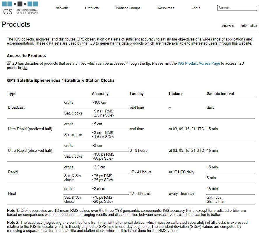
This system is augmented by other tracking networks that produce post-computed ephemerides. Their impetus have been several: the necessity of timely orbital information with more precision than the broadcast ephemeris and the correlation of the terrestrial coordinate systems with the orbital system through VLBI and SLR sites, among others. Since the monitoring stations are tracking the actual satellites all the time, it is possible this tracking information can be used to produce ephemerides of the actual position of the satellite at the time you were observing it. In other words, given a position on the Earth and given a window of time, it is possible for you to go on the Internet and download from these sites the precise ephemeris, the post-computed ephemeris, of the moment at which you were observing the satellite. It's valuable, of course, because the broadcast ephemeris is not as accurate as the tracking information of the actual satellites you're observing at the time you're observing them. The broadcast ephemeris is predictive of where the satellite will be later. It is much different to have the tracking information of the satellite at the moment you were tracking it with your receiver.
The following ephemeris categories and the time they are available after tracking (latency) can be found at NOAAs GPS Orbit Data site
Ultra-rapid (iguWWWWD.sp3)
6-hour latency
constrained (no-net rotation, no-net translation) 24-hour file – sp3
Rapid (igrWWWWD.sp3)
13-hour latency
constrained (no-net rotation, no-net translation) 24-hour file – sp3
Final (igsWWWWD.sp3)
12 to 14 day latency
minimally constrained (no-net rotation) 24 hour file - sp3
Discussion
Discussion Instructions
To continue the discussion begun by this lesson, I would like to pose this question:
In a properly designed static GPS/GNSS survey would a loop closure include independent or dependent baselines? What is the difference between independent and dependent baselines? Why is redundancy a good thing in GPS/GNSS work?
To participate in the discussion, please go to the Lesson 7 Discussion Forum in Canvas. (That forum can be accessed at any time by going to the GEOG 862 course in Canvas and then looking inside the Lesson 7 module.)
Summary
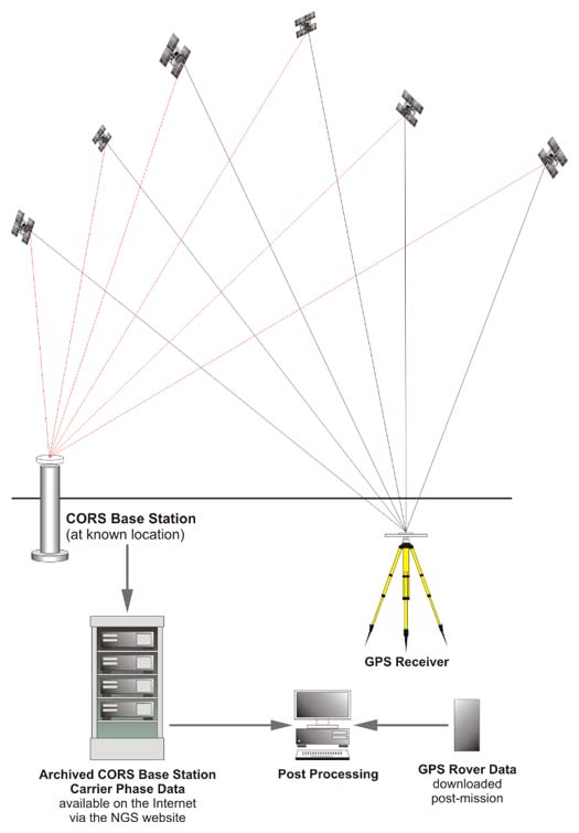
So, here are the fundamental ideas that underlie the static GPS/GNSS surveying technique. The first receiver, the base, provides the data to compute the differences between its known position and the unknown positions measured at the second, or roving receiver. Static GPS/GNSS requires post-processing and is used for establishing control by GPS/GNSS. While correlated systematic errors can be virtually eliminated with differential correction, the biases such as multipath and receiver channel noise are certainly not. These errors have been much reduced in modern GPS/GNSS receivers, but not completely defeated. Biases such as high PDOP can only be resolved with both good receiver design and care as to when and where the surveying is done.
In the next lesson, we delve into real-time GPS/GNSS work and Precise Point Positioning.
Before you go on to Lesson 8, double-check the Lesson 7 Checklist to make sure you have completed all of the activities listed there.