Lesson 9: GPS Modernization
The links below provide an outline of the material for this lesson. Be sure to carefully read through the entire lesson before returning to Canvas to submit your assignments.
Lesson 9 Overview
Overview
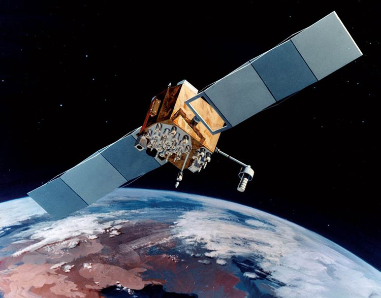
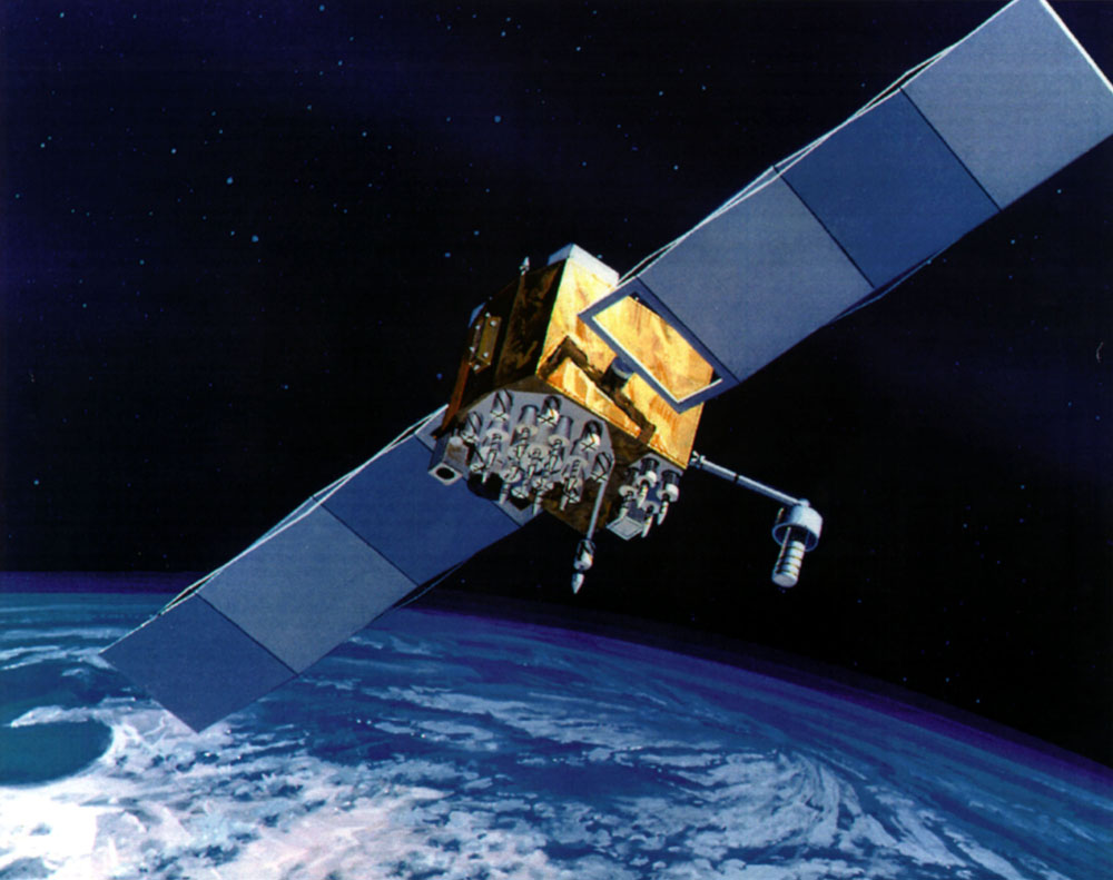
The configuration of the GPS Space Segment is well-known. A minimum of 24 GPS satellites ensure 24-hour worldwide coverage. But, today, there are more than that minimum on orbit. There are a few spares on hand in space. The redundancy is prudent. GPS, put in place with amazing speed considering the technological hurdles, is now critical to all sorts of positioning, navigation, and timing around the world. It’s that very criticality that requires the GPS modernization. The oldest satellites in the current constellation were launched in 1989. Imagine using a personal computer of that vintage today. It is not surprising that there are plans in place to alter the system substantially. What might be unexpected is many of those plans will be implemented entirely outside of the GPS system itself.
Objectives
At the successful completion of this lesson, students should be able to:
- recognize GPS Modernization;
- explain the difference between Block I, Block II, Block IIR, Block IIR-M, BLock IIF and Block III satellites;
- describe power spectral density diagrams;
- identify the M Code;
- define L2C;
- recognize L5;
Questions?
If you have any questions now or at any point during this week, please feel free to post them to the Lesson 9 Discussion Forum. (To access the forum, return to Canvas and navigate to the Lesson 9 Discussion Forum in the Lesson 9 module.) While you are there, feel free to post your own responses if you, too, are able to help out a classmate.
Checklist
Lesson 9 is one week in length. (See the Calendar in Canvas for specific due dates.) To finish this lesson, you must complete the activities listed below. You may find it useful to print this page out first so that you can follow along with the directions.
| Step | Activity | Access/Directions |
|---|---|---|
| 1 | Read the lesson Overview and Checklist. | You are in the Lesson 9 online content now. The Overview page is previous to this page, and you are on the Checklist page right now. |
| 2 | Read "Global Positioning System Modernization and Global Navigation Satellite Systems" pages 267 to 284 in Chapter 8 in GPS for Land Surveyors. | Text |
| 3 | Read the lecture material for this lesson. | You are currently on the Checklist page. Click on the links at the bottom of the page to continue to the next page, to return to the previous page, or to go to the top of the lesson. You can also navigate the lecture material via the links in the Lessons menu. |
| 4 | Participate in the Discussion. | To participate in the discussion, please go to the Lesson 9 Discussion Forum in Canvas. (That forum can be accessed at any time by going to the GEOG 862 course in Canvas and then looking inside the Lesson 9 module.) |
| 5 | Read lesson Summary. | You are in the Lesson 9 online content now. Click on the "Next Page" link to access the Summary. |
GPS Modernization
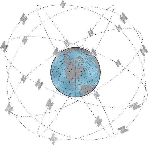
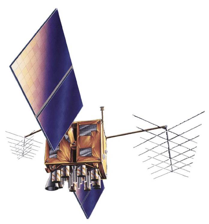
The configuration of the GPS Space Segment is well known. The satellites are on orbit at a nominal height of about 20,000 km above the Earth. There are three carriers L1 (1575.42 MHz), L2 (1227.60 MHz), and L5 (1176.42 MHz). A minimum of 24 GPS satellites ensure 24-hour worldwide coverage, but there are more than that minimum on orbit. There are a few spares on hand in space. The redundancy is prudent because GPS is critical to positioning, navigation and timing. It is also critical to the smooth functioning of financial transactions, air traffic, ATMs, cell phones, and modern life in general around the world. This very criticality requires continuous modernization.
GPS was put in place with amazing speed considering the technological hurdles and reached its Fully Operational Capability (FOC) on July 17, 1995. The oldest satellites in the current constellation were launched in the late 1990s. If you imagine using a personal computer of that vintage today, it is not surprising that there are plans in place to alter the system substantially. In 2000, U.S. Congress authorized the GPS III effort. The project involves new ground stations and satellites, additional civilian and military navigation signals, and improved availability. This chapter is about some of the changes in the modernized GPS, its inclusion in the Global Navigation Satellite System and more. Block I GPS SatelliteBlocks I and II GPS Satellitesthe design life has obviously been exceeded in most cases, Block IIA satellites do wear out. Block IIR GPS Satellite.
Satellite Blocks
Block I
| Demonstrated GPS |
|---|
|
The 11 GPS satellites launched from Vandenberg Air Force Base between 1978 and 1985 were known as Block I satellites. The last Block I satellite was retired in late 1995. Ten of the satellites built by Rockwell International achieved orbit on Atlas F rockets. There was one launch failure. All were prototype satellites built to validate the concept of GPS positioning. This test constellation of Block I satellites was inclined by 63° to the equator instead of the current specification of 55°. They could be maneuvered by hydrazine thrusters operated by the control stations.
The first GPS satellite was launched February 22, 1978 and was known as Navstar 1. An unfortunate complication is that this satellite was also known as PRN 4 just as Navstar 2 was known as PRN 7. The Navstar number, or Mission number includes the Block name and the order of launch, for example I-1, meaning the first satellite of Block I. and the PRN number refers to the weekly segment of the P code that has been assigned to the satellite, and there are still more identifiers. Each GPS satellite has a Space Vehicle number, an Interrange Operation Number, a NASA catalog number, and an orbital position number as well. However, in most literature, and to the GPS receivers themselves, the PRN number is the most important.
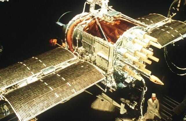
Continuing the discussion of the space segment, here is the Block 1 satellite. These were the first launched. There are none of them functional today. But they certainly did an extraordinary job in getting the system started. It was an experimental system at that time. But it certainly has worked out well.
The Block I satellites weigh 845 kg in final orbit. They were powered by three rechargeable nickel-cadmium batteries and 7.25 square meters of single-degree solar panels. These experimental satellites served to point the way for some of the improvements found in subsequent generations. For example, even with the back-up systems of rubidium and cesium oscillators onboard each satellite, the clocks proved to be the weakest components. The satellites, themselves, could only store sufficient information for 3½ days of independent operation. And the uploads from the control segment were not secure; they were not encrypted. Still, all 11 achieved orbit, except Navstar 7. The design life for these satellites was 4½ years, but their actual average lifetime was 8.76 years. That is something that continues. The GPS satellites have mostly outlived their design life. There are no Block I satellites operating today.
Block II
| Some of the iMprovements over Block I |
|---|
|
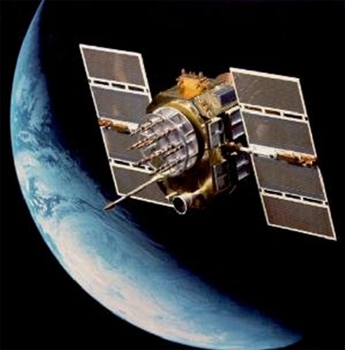
The next generation of GPS satellites are known as Block II satellites. The first left Cape Canaveral on February 14, 1989, almost 14 years after the first GPS satellite was launched. It was about twice as heavy as the first Block I satellite and was expected to have a design life of 7½ years with a Mean Mission Duration, MMD of 6 years. The Block II satellites could operate up to 14 days without an upload from the control segment and their uploads were encrypted. The satellites themselves were radiation hardened, and their signals were subject to selective availability.
These satellites were built by Rockwell International. Block II included the launch of 9 satellites between 1989 and 1990. None of the Block II satellites are in the constellation today. the last was decommissioned in 2007
Block IIA
| Some of the iMprovements over Block II |
|---|
|
The launch of the Block IIA satellites began in 1990. 19 Block IIA satellites, with several navigational improvements, were launched between 1990 and 1997. Block IIA satellites could store more of the Navigation message than the Block II satellites, and could, therefore, operate without contact with the Control Segment for 6 months. However, if that were actually done, their broadcast ephemeris and clock correction would have degraded. None of the Block IIA satellites are in the constellation today.
Block IIR
| Some of the iMprovements over Block IIA |
|---|
|
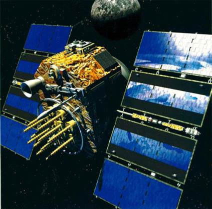
The first launch of the next Block, Block IIR satellites in January of 1997 was unsuccessful. The following launch in July of 1997 succeeded. The third generation of GPS satellites is known as Block IIR satellites, the R stands for replenishment. There are two significant advancements in these satellites. The Block IIR satellites have enhanced autonomous navigation capability because of their use of intersatellite linkage (called AutoNav). This involves their use of reprogrammable processors onboard to do their own fixes in flight. There are Block IIR satellites in the constellation today.
Block IIR-M
| Some of the iMprovements over Block IIR |
|---|
|
In September of 2005, the first of the next improved block, called Block IIR-M was launched. These are IIR satellites that were modified before they were launched. The modifications upgraded these satellites so that they radiate two new codes; a new military code, the M code, a new civilian code, the L2C code, and demonstrate a new carrier, L5. There are Block IIR-M satellites in the constellation today.
Block IIF

| Some of the iMprovements over Block IIR-M |
|---|
|
The L2C signal and the third civilian carrier will be very helpful because, as you know, ionosphere modeling is an important part of error management in GPS. We can model it to some good degree with two carriers. Three will obviously make that modeling even better.
Block IIF is the most recent group of GPS satellites launched and the first of them reached orbit in May of 2010. There has been steady and continuous improvement in the GPS satellite constellation from the beginning.
The first Block IIF satellite was launched in the summer of 2010. Their design life is 12 to 15 years. Block IIF satellites have faster processors and more memory onboard. They broadcast all of the previously mentioned signals including the L5 carrier, This signal was demonstrated on the Block IIR-M and is available from all of the Block IIF satellites. The Block IIF satellites replaced the Block IIA satellites as they aged. Their onboard navigation data units (NDU) support the creation of new navigation messages with improved broadcast ephemeris and clock corrections. Like the Block IIR satellites, the Block IIF can be reprogrammed on orbit.
Block III

| Some of the iMprovements over Block IIF |
|---|
|

The Legacy Signals and Power Spectral Density Diagrams
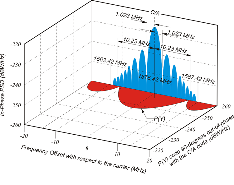
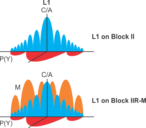
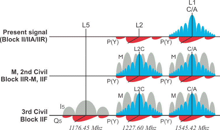
The Power Spectral Density (PSD) diagrams show the increase or decrease, in decibels, of power in Watts with respect to frequency in Hertz. It allows you to see some of the things we've already discussed. For example, this is the C/A Code in the blue on the L1 carrier, which, of course, is centered at 1,575.42 megahertz and then spread over a bandwidth that is spread spectrum. It's about 10.23 megahertz on each side for a total of like 20.46. That in the red, you see the P(Y) Code is in quadrature 90 degrees from the C/A Code. It has really one main lobe and then two sidebands, and then the blue C/A Code has many lobes.
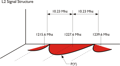
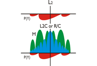
The L2 signal diagram is centered on 1,227.60 MHz. As you can see, it is similar to the L1 diagram except for the absence of the C/A code which is, of course, not carried on the L2 frequency. As well-known as these are, this state of affairs is changing.
Power Spectral Density Diagrams
Many of the improvements in GPS are centered on the broadcast of new signals. Therefore, it is pertinent to have a convenient way to visualize all the GPS and GNSS signals that illustrate the differences in the new signals and a good deal of signal theory as well. It is a diagram of the power spectral density function (PSD). They graphically illustrate the signal's power per bandwidth in Watts per Hertz as a function of frequency. In GPS and GNSS literature, the PSD diagram is often represented with the frequency in MHz on the horizontal axis and the density, the power, represented on the perpendicular axes in decibels relative to one Hertz per Watt or dBW/Hz.
The actual definition of PSD is the Fourier transform of the autocorrelation function, but the idea behind them is to give you an idea of the power within a signal with regard to frequency. These graphics show the increase or decrease, in decibels, of power, in Watts with respect to frequency in Hertz, of the well-known signals on L1 and L2.
dBW/Hz
Perhaps a bit of background is in order to explain those units. A bel unit originated at Bell Labs to quantify power loss on telephone lines. A decibel is a tenth of a bel. A decibel, dB, is a dimensionless number. In other words, it's a ratio that can acquire dimension by being associated with measured units. A change of 1 decibel would be an increase or a decrease of 27 percent. A change of 3 decibels would be an increase or a decrease of 100 percent. Here are some of the quantities with which it is sometimes associated: seconds of time, symbolized dBs, bandwidth measured in Hertz, symbolized dBHz, and temperature measured in Kelvins, symbolized dBK. Since signal power is of interest here, dB will be described with respect to 1Watt, the symbol used is dBW.
dBW is a short, concise number that can conveniently express the wide variation in GPS signal power levels. dBW can represent quite large and quite small amounts of power more handily than other notations. For example, consider a value of interest in GPS signals. The value is very small, one tenth of a millionth billionth of a watt. Expressing it as 0.0000000000000001 W is a bit exhausting. It would be more convenient expressed in dBW, a value that can be derived using the formula.
where is the power of the signal.
The expression -160 dBW is immediately useful. Here's an example. A change in 3 decibels is always an increase or a decrease of 100% in power level. Stated another way, a 3-decibel increase indicates a doubling of signal strength and a 3-decibel decrease indicates a halving of signal strength. Therefore, it is easy to see that a signal of -163 dBW has half the power of a signal of -160dBW. Considering the broadcasts from the current constellation of satellites, the minimum power received from the P code on L1 by a GPS receiver on the Earth's surface is about -163 dBW, and the minimum power received from the C/A code on L1 is about -160dBW. This difference between the two received signals is not surprising, since at the start of their trip to Earth they are transmitted by the satellite at power levels that are also 3 decibels apart. The P code on L1is transmitted at a nominal +23.8 dBW (240 W), whereas the nominal transmitted power of the C/A code on L1 is +26.8 dBW (479 W). It is interesting to note that the minimum received power of the P code on L2 is even less at -166 dBW, and its nominal transmitted power is +19.7 dBW (93 W).
One might wonder why there are such differences between the power of the transmitted GPS signal, called the Effective Isotropic Radiated Power (EIRP), and the power of the received signal. The difference is large. It is 186 to 187 dB, nearly 10 quintillion decibels. The loss is mostly because is the 20,000 km distance from the satellite to a GPS receiver on the Earth. There is also an atmospheric loss and a polarization mismatch loss, but the biggest loss by far, about 184 dB, is along the path in free space.
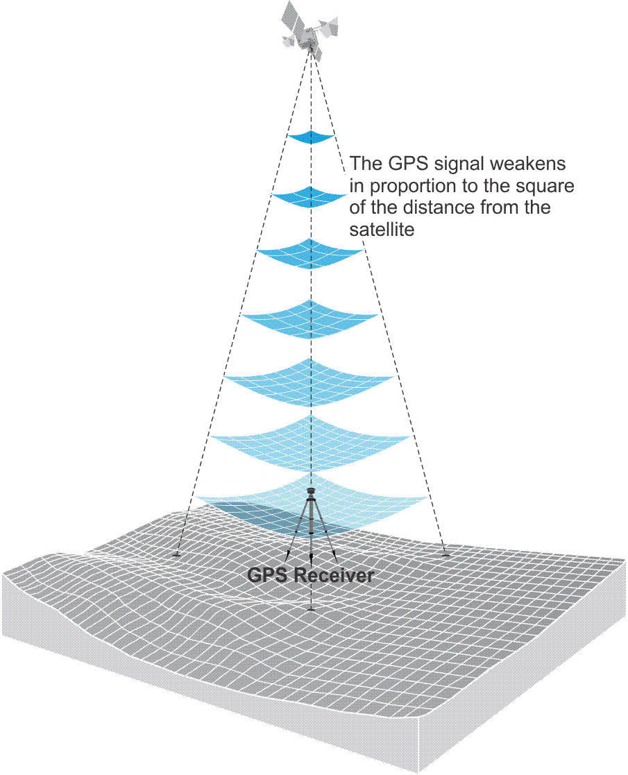
Much of this loss is a function of the spreading out of the GPS signal in space, as described by the inverse square law. The intensity of the GPS signal varies inversely to the square of the distance from the satellite. In other words, by the time the signal makes that trip and reaches the GPS receiver, it is pretty weak, as shown in the 'Inverse Square Law' figure above (Figure 8.3 from the textbook). It follows that GPS signals are easily degraded by vegetation canopy, urban canyons, and other interference.
A GPS signal has power, of course, but it also has bandwidth. PSD is a measure of how much power a modulated carrier contains within a specified bandwidth. That value can be calculated using the following formula and allowing that there is an even distribution of 10-16 W over the 2.046 MHz C/A bandwidth of the C/A code:
The calculation is also frequently normalized and done presuming an even distribution of 1W over the 2.046 MHz C/A bandwidth of the C/A code. In other words, the following calculation presumes an even distribution of the power over 1W instead of the 10-16 W used in the previous calculation:
The M-Code

New Signals
An important aspect of GPS modernization is the advent of some new and different signals that are augmenting the old reliable codes. In GPS, a dramatic step was taken in this direction on September 21, 2005 when the first Block IIR-M satellite was launched. One of the significant improvements coming with the Block IIRM satellites is increased L-band power on both L1 and L2 by virtue of the new antenna panel. The Block IIR-M satellites will also broadcast new signals, such as the M-code.
The M-Code
Eight to twelve of these replenishment satellites are going to be modified to broadcast a new military code, the M-code. This code will be carried on both L1 and L2 and will probably replace the P(Y) code eventually. It has the advantage of allowing the Department of Defense (DoD) to increase the power of the code to prevent jamming. There was consideration given to raising the power of the P(Y) code to accomplish the same end, but that strategy was discarded when it was shown to interfere with the C/A code.
The M-code was designed to share the same bands with existing signals, on both L1 and L2, and still be separate from them. See those two peaks in the M-code in the illustration. They represent a split-spectrum signal about the carrier. Among other things, this allows minimum overlap with the maximum power densities of the P(Y) code and the C/A code, which occur near the center frequency. That is because the actual modulation of the M-code is done differently. It is accomplished with binary offset carrier (BOC) modulation, which differs from the binary phase shift key (BPSK) used with the legacy C/A and P(Y) signals. As a result of this BOC modulation, the M-code has its greatest power density at the edges, which is at the nulls, of the L1 away from P(Y) and C/A. This architecture both simplifies implementation at the satellites and receivers and also mitigates interference with the existing codes. Suffice it to say that this aspect and others of the BOC modulation strategy offer even better spectral separation between the M-code and the older legacy signals.
The M-code is unusual in that a military receiver can determine its position with the M-code alone, whereas with the P(Y) it must first acquire the C/A code to do so. It is also spread across 24 MHz of the bandwidth.
Perhaps it would also be useful here to mention the notation used to describe the particular implementations of the Binary Offset Carrier. It is characteristic for it to be written BOC (α, ß). Here the α indicates the frequency of the square wave modulation of the carrier, also known as the subcarrier frequency factor. The ß describes the frequency of the pseudorandom noise modulation, also known as the spreading code factor. In the case of the M-code, the notation BOC (10, 5) describes the modulation of the signal. Both here are multiples of 1.023 MHz. In other words, their actual values are.
.
The M-code is tracked by direct acquisition. This means that, as mentioned in Lesson 1, the receiver correlates the signal coming in from the satellite with a replica of the code that it has generated itself.
One of the significant improvements coming from the Block IIR-M satellites is increased L band power on both L1 and L2. This new M-Code will possibly replace the P-Code, eventually. It will be carried on both L1 and L2, and it has an advantage that the Department of Defense can increase the power of the code to prevent jamming. There was consideration to raising the power of the Y-Code to accomplish the same end, but that was discarded when it was shown to interfere with the C/A Code. So to recap, the M-Code will be carried on L1 and L2, but because of the binaries offset carrier modulation, it will not interfere with the older legacy codes, the C/A Code and P-Code.
L2C and CNAV
L2 Signal
In the illustration, the L2 signal diagram is centered on 1227.60 MHz. As you can see, it is similar to the L1 diagram except for the absence of the C/A code, which is, of course, not carried on the L2 frequency. As well-known as these are, this state of affairs is changing. We have been using the L2 carrier since the beginning of GPS, of course, but there will be two new codes broadcast on the carrier, L2, that previously only carried one military signal exclusively, the P(Y) code. L2 will carry a new military signal, the M-code, just discussed, and a new civil signal as well.
On the upper portion of this diagram, you see the L2 carrier, of course, with only the P-Code encrypted as the Y-Code. In the lower part, there is the same L2 with P-Code, but the M-Code is included, and there's a new civilian code. This one is called L2C. Before this, there was no civilian code on L2. There was only the C/A Code on L1. However, these new IIR-M satellites will be carrying the L2C, a civil code on L2. We've been using the L2 carrier since the beginning of GPS, of course, but there will be two new codes broadcast on that carrier, the M-Code and the new Civilian code L2C.
L2C
A new military code on L1 and L2 may not be terribly exciting to civilian users, but these IIR-M satellites have something else going for them. They broadcast a new civilian code. We have been using the L2 carrier since the beginning of GPS of course, but there will be two new codes broadcast on the carrier, L2, that previously only carried one military signal, the P(Y) code. L2 will carry the new military signal, the M-code, and a new civil signal as well. This is a code that was first announced back in March of 1998. It is transmitted by all block IIR-M satellites and subsequent blocks and is known as L2C. The “C” is for civil.
Even though its 2.046 MHz from null-to-null gives it a very similar power spectrum to the C/A code, it is important to note that L2C is not a copy of the C/A-code even though that was the original idea. The original plan was that it would be a replication of the venerable C/A code, but carried on L2 instead of L1. This concept changed when Colonel Douglas L. Loverro, Program Director for the GPS Joint Program Office (JPO), was asked if perhaps it was time for some improvement of C/A. The answer was yes. The C/A code is somewhat susceptible to both waveform distortion and narrow-band interference, and its cross-correlation properties are marginal at best. So, the new code on L2, known as L2 civil, or L2C was announced. It is more sophisticated than C/A. So, the L2C is actually a different code than the C/A. Still, it's a civilian accessible code, and it's carried on L2 instead of L1.
Civil-Moderate (CM) and Civil-Long (CL)
L2C is actually composed of two pseudorandom noise signals: the civil-moderate length code, CM, and the civil long code, CL. They both utilize the same modulation scheme, binary phase shift key (BPSK), as the legacy signals, and both signals are broadcast at 511.5 kilobits per second (Kbps). This means that CM repeats its 10230 chips every 20 milliseconds, and CL repeats its 767250 chips every 1.5 seconds. But, wait a minute, how can you do that? How can you have two codes in one?
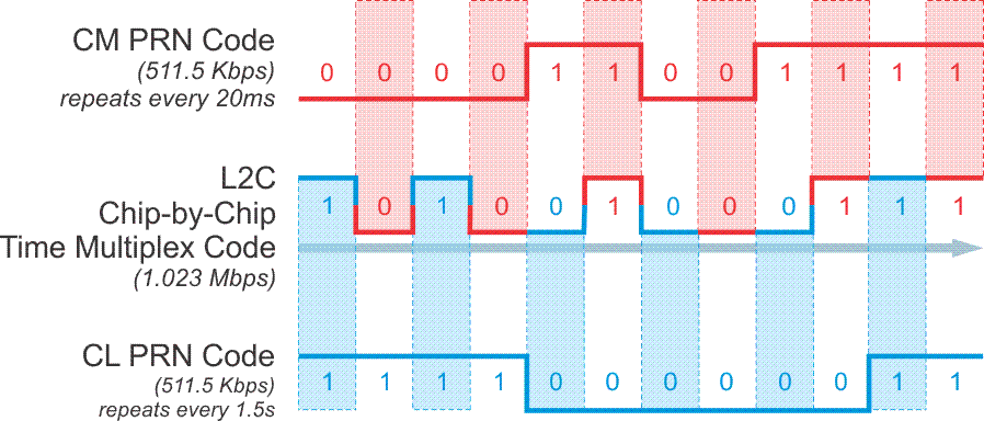
L2C achieves this by time multiplexing. Since the two codes have different lengths L2C alternates between chips of the CM code and chips of the CL code as shown in the illustration. It is called chip-by-chip time multiplexing. So, even though the actual chipping rate is 511.5 KHz, half the chipping rate of the C/A code, with the time multiplexing it still works out that taken together L2C ends up having the same overall chip rate as L1 C/A code, 1.023 MHz . This provides separation from the M code.
In this illustration, I try to answer the question how it's possible in L2C to have two codes, the CM Code and the CL Code, simultaneously operating on the same signal. It's known as multiplexing, and we discussed that briefly when we were talking about receivers, except, in this case, it's chip by chip time multiplexing. The CM Code, the moderate length code, goes through 10,238 chips before it repeats. It repeats every 20 milliseconds, but the CL Code, the long code, repeats after 1.5 seconds.
Those lengths give you very good cross correlation protection. In fact, both are longer than the C/A Code and present a subsequent improvement in autocorrelation. This is because the longer the code, the easier it is to keep the desired signal separate from the background. In practice, this means that these signals can be acquired with more certainty by a receiver which can maintain locking them more surely in marginal situations where the sky is obstructed.
So, it is possible to have these two signals, the CM and the CL on the L2C because the receiver can shift back and forth between the two with good, solid cross correlation and lock on to the signals even in circumstances where the sky is obstructed better than one can with the C/A Code. It's important to note that the L2C is actually slightly weaker, 2.3 decibels weaker, than the C/A Code. And it's surprising that this is not a disadvantage, because the receiver can track the long dataless CL, that's the long code on L2C with the phase locked loop instead of squaring Costas loop.
In other words, the long dataless sequence of the CL provides for correlation that is actually about 250 times stronger than the C/A Code. So, despite the fact that its transmission power is 2.3 decibels weaker compared to the C/A Code, the L2C has 2.7 decibels greater data recovery and 0.7 decibels greater carrier tracking. It's actually more solid, even though the power is slightly less.
L2C has better autocorrelation and cross-correlation protection than the C/A code because both of the CM and CL codes are longer than the C/A code. Longer codes are easier to keep separate from the background noise. In practice, this means these signals can be acquired with more certainty by a receiver that can maintain lock on them more surely in marginal situations where the sky is obstructed.
There is also another characteristic of L2C that pays dividends when the signal is weak. While CM carries newly formatted navigation data and is, therefore, known as the data channel, CL does not. It is dataless and known as a pilot channel. A pilot channel can support longer integration when the signal received from the satellite is weak. This is an idea that harks all the way back to Project 621B at the very beginnings of GPS. The benefits of a pilot channel distinct from the data components carried by a signal was known in the 1960s and 1970s but was not implemented in GPS until recently.
Phase-Locked Loop
Even though the L2C signals’ transmission power is 2.3 dB weaker than is C/A on L1, and even though it is subject to more ionospheric delay than the L1 signal, L2C is still much more user friendly. The long data-less CL pilot signal has 250 times (24dB) better correlation protection than C/A. This is due in large part to the fact that the receiver can track the long data-less CL with a phase-locked loop instead of a squaring Costas loop that is necessary to maintain lock on CM, C/A and P(Y). This allows for improved tracking from what is, in fact, a weaker signal and a subsequent improvement in protection against continuous wave interference. As a way to illustrate how this would work in practice, here is one normal sequence by which a receiver would lock onto L2C. First, there would be acquisition of the CM code with a frequency locked or Costas loop, next there would be testing of the 75 possible phases of CL, and finally acquisition of CL. The CL, as mentioned, can be then tracked with a basic phase-locked loop. Using this strategy, even though L2C is weaker than C/A there is actually an improvement in the threshold of nearly 6 dB by tracking the CL with the phase-locked loop. Compared to the C/A code L2C has 2.7 dB greater data recovery and 0.7 dB greater carrier-tracking.
Practical Advantages
Great, so what does all that mean in English? Having two civilian frequencies being transmitted from one satellite affords the ability to model and lessen the ionospheric delay error for that satellite while relying on code phase pseudorange measurements alone. In the past, ionospheric modeling was only available to multi carrier frequency observations, or by reliance on the atmospheric correction in the Navigation message. Before May 2, 2000 with Selective Availability on a code-based receiver could get you within 30 to 100 meters of your true position; when SA was turned off, that was whittled down to 15 to 20 meters or so under very good conditions. But with just one civilian code C/A on L1, there was no way to remove the second largest source of error in that position, the ionospheric delay.
But with two civilian signals, one on L1 (C/A) and one on L2 (L2C), it becomes possible to effectively model the ionosphere using code phase. In other words, it may become possible for an autonomous code-phase receiver to achieve positions with a 5-10m positional accuracy with some consistency.
The L2C signal also ameliorates the effect of local interference. This increased stability means improved tracking in obstructed areas like woods, near buildings, and urban canyons. It also means fewer cycle slips.

With L2C, there will be a better tolerance for interference, increased stability, and fewer cycle slips. That means that GPS will work better in obstructed areas, and this will be a practical advantage to those like the fellow with his receiver looking up to an obstructed sky. A second civilian code on a separate frequency is another really practical advantage. You can model the ionosphere with a multi-frequency receiver because of the dispersive characteristic of the ionosphere. However, those that have been operating purely in code phase or pseudo range positions have not had that advantage. Now, with L2C on L2, and C/A Code on L1, there will be two civilian accessible codes available to a code phase pseudo range receiver making it possible to model the ionosphere with a code observation. This should improve the positions available from purely code phase receivers quite a bit.
So, even if it is the carrier-phase that ultimately delivers the wonderful positional accuracy we all depend on, the codes get us in the game and keep us out of trouble every time we turn on the receiver. The codes have helped us to lock on to the first satellite in a session and allowed us to get the advantage of cross-correlation techniques almost since the beginning of GPS. In other words, our receivers have been combining pseudorange and carrier-phase observables in innovative ways for some time to measure the ionospheric delay, detect multipath, do wide laning, and so forth. But those techniques can be improved, because while the current methods work, the results can be noisy and not quite as stable as they might be, especially over long baselines. It will be cleaner to get the signal directly once there are two clear civilian codes, one on each carrier. It may also help reduce the complexity of the chipsets inside our receivers, and might just reduce their cost as well.
Along that line, it is worthwhile to recall that the L2C has an overall chip rate of 1.023 MHz, just like L1 C/A. Such a slow chip rate can seem to be a drawback until you consider that that rate affects the GPS chipset power consumption. In general, the slower the rate, the longer the battery life, and the improvement in receiver battery life could be very helpful. And not only that, the slower the chip rate, the smaller the chipset. That could mean more miniaturization of receiver components.
L2C is clearly going to be good for the GPS consumer market, but it also holds promise for surveyors. Nevertheless, there are a few obstacles to full utilization of the L2C signal. It will be some time before the constellation of Block IIR-M necessary to provide L2C at an operational level is up and functioning. Additionally, aviation authorities do not support L2C. It is not in an Aeronautical Radionavigation Service (ARNS) protected band. It happens that L2 itself occupies a radiolocation band that includes ground-based radars.
Click here to see a text description.
| Messages (pseudo-packetized) | 1 Word | 2 Words | 3-10 Words |
|---|---|---|---|
| 0 | MT | How | Default |
| 10 | MT | How | Ephemeris 1 |
| 11 | MT | How | Ephemeris 2 |
| 13 | MT | How | Clock Differential Correction |
| 14 | MT | How | Ephermis Differential Correction |
| 15 | MT | How | Text |
| 30 | MT | How | Clock, IONO, &Group Delay |
| 31 | MT | How | Clock & Reduced Almanac |
| 63 | MT | How | MT7-67 still to be defined |
CNAV
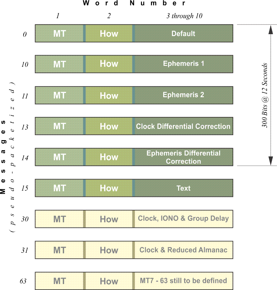
The navigation data on CM portion of the L2C signal is improved over the legacy Navigation message. It is called CNAV. It was tested using some of the message types, MT, shown in the illustration in June of 2013.
You may recall that the legacy Navigation message was mentioned in Chapter 1. It is also known by the acronym NAV. The information in CNAV is fundamentally the same as that in the original NAV message, but there are differences. It includes the almanac, ephemerides, time, and satellite health. CNAV contains 300-bit messages like the legacy NAV message, but CNAV packages its 12-second, 300-bit messages differently. Instead of the repetition of frames and sub-frames in a fixed pattern as is the case with the legacy NAV, CNAV utilizes a pseudo-packetized message protocol. One of every four of these packets includes clock data; two of every four contains ephemeris data, and so on. This makes CNAV more flexible than NAV. The order and the repetition of the individual messages in CNAV can be varied. CNAV can accommodate the transmission of the information in support of 32 satellites using 75% or less of its bandwidth. CNAV is also more compact than NAV, and that allows a receiver to get to its first fix on a satellite much faster.
A packet in message 35 of CNAV was assigned to the time offset between GPS and GNSS in the June 2013 test. Such a message would be a boon for interoperability between GPS, Galileo, and GLONASS. Also, each packet contains a flag which can be toggled on within a few seconds of the moment a satellite is known to be unhealthy. This is exactly the sort of quick access to information necessary to support safety-of-life applications. Only a fraction of the available packet types are being used at this point. CNAV is designed to grow, and can accommodate 63 satellites as the system requires. For example, there could be packets that would contain differential correction like that available from satellite-based augmentation systems (SBAS).
There is also a very interesting aspect to the data broadcast on CM known as Forward Error Correction (FEC). An illustration of this technique is to imagine that every individual piece of data is sent to the receiver twice. If the receiver knows the details of the protocol to which the data ought to conform, it can compare each of the two instances it has received to that protocol. If they both conform, there is no problem. If one does and one does not, the piece of data that conforms to the protocol is accepted and the other is rejected. If neither conforms, then both are rejected. Using FEC allows the receiver to correct transmission errors itself, on the fly. FEC will ameliorate transmission errors and reduce the time needed to collect the data.
There is a packet in CNAV that may be assigned to the time offset between GPS and GNSS. So, one of the things we'll talk about is that GLONASS's time standard is different than that of GPS, and the difference can be loaded into the navigation message, so there's some preparation here for the GNSS future. Each packet contains a flag that can be turned on and off very quickly to indicate that a satellite is unhealthy. This could be quite useful for safety of life, things such as ambulances and so on. Because if a satellite should not be used in positioning if it will corrupt the results, it's important to know that immediately in real time. It's great to have a system that can provide that.
L5
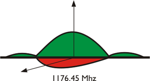
Alright, L2C is fine, but what about L5, the new carrier being broadcast on the Block IIF satellites? It is centered on 1176.45 MHz, 115 times the fundamental clock rate.
As you see from the illustration, the basic structure of L5 looks similar to that of L1. There are two pseudorandom noise (PRN) codes on this 20 MHz carrier. The two codes are modulated using Quad Phase Shift Key (QPSK), and they are broadcast in quadrature to each other. However, borrowing a few pages from other recent developments, the in-phase (I) signal carries a data message that is virtually identical to the CNAV on L2. The other, the quadraphase signal (Q), is data-less and L5 utilizes chip-by-chip time multiplexing in broadcasting its two codes, as does L2C in broadcasting CM and CL.
Both L5 codes have a 10.23 MHz chipping rate, the same as the fundamental clock rate. This is the same rate that has been available on the P(Y) code from the beginning of the system. However, this is the fastest chipping rate available in any civilian code. L5 has the only civilian codes that are both ten times longer and ten times faster than the C/A code. Since the maximum resolution available in a pseudorange is typically about 1% of the chipping rate of the code used, the faster the chipping rate, the better the resolution.
L5 has about twice as much power as L1, and since L5 does not carry military signals, it achieves an equal power split between its two signals. In this way, L5 lowers the risk of interference and improves multipath protection. It also makes the data-less signal easier to acquire in unfavorable and obstructed conditions.
Unlike L2C, L5 users will benefit from its place in a band designated by the International Telecommunication Union (ITU) for the Aeronautical Radionavigation Navigation Services (ARNS) worldwide. Therefore, it is not prone to interference with ground based navigation aids and is available for aviation applications. While no other GPS signal occupies this band, L5 does share space with one of the Galileo signals, E5. L5 does also incorporate Forward Error Correction (FEC).
It is helpful that L5 will share space with one of the E5A signal from an entirely separate satellite system, Galileo. This is the European contribution to GNSS. The fast chipping rate on L5 is also good news.
Block IIF and Block III
The first Block IIF satellite was launched in the summer of 2010. As of 2014. There are 12 Block IIF satellites on orbit. Their design life is 12 to 15 years. Block IIF satellites have faster processors and more memory onboard. They broadcast all of the previously mentioned signals, and one more, a new carrier known as L5. This is the signal that was demonstrated on the Block IIR-M. It is available from all of the Block IIF satellites. The L5 signal is within the Aeronautical Radio Navigation Services (ARNS) frequency and can service aeronautical applications. The improved rubidium frequency standards on Block IIF satellites have a reduced white noise level. The Block IIF satellite's launch vehicles can place the satellites directly into their intended orbits, so they do not need the apogee kick motors their predecessors required. All of the Block IIF satellites will carry DASS repeaters. Their onboard navigation data units (NDU) support the creation of new navigation messages with improved broadcast ephemeris and clock corrections. The Block IIF can be reprogrammed on orbit.

Block III satellite
There are currently 3 Block IIIA satellites on orbit and operational. They broadcast all of the previously mentioned signals and one more, L1C.
Summary of C/A, L2C, and L5
GPS modernization is underway. New spacecraft with better electronics, better navigation messages, newer and better clocks are just part of the story. Beginning with the launch of the first IIR-M satellite, new civil signals began to appear, starting with L2C which was followed by L5 on the Block IIF satellites.
These signals tend to have longer codes, faster chipping rates, and more power than the C/A and P(Y) codes have. In practical terms, these developments lead to faster first acquisition, better separation between codes, reduced multipath and better cross-correlation properties.
The legacy L1 and L2 signals are at the top of the illustration. In the next tier, you see the L1 with the addition of the M-Code and substantially the same otherwise. L2 has both the M-Code and the new L2C Civilian code. In the third tier and the Block IIF satellites, there is the addition of L5.
New Signal Availability and Some Benefits
| Carrier | Signal | Block IIR | Block IIR-M | Block IIF |
|---|---|---|---|---|
| L1 | P/Y | ⦿ | ⦿ | ⦿ |
| L2 | P/Y | ⦿ | ⦿ | ⦿ |
| L1 | CA | ⦿ | ⦿ | ⦿ |
| L2 | L2C | ⦿ | ⦿ | |
| L1 | M | ⦿ | ⦿ | |
| L2 | M | ⦿ | ⦿ | |
| L5 | Civil | ⦿ |
In the table, you see that the Block IIR-M satellites have the addition of the M-Code and the L2C to the legacy signals available from the Block IIR satellites. The Block IIF satellites IIFs have all the previous codes and L5.
Ionospheric Bias
Concerning the effect of the ionosphere—as you know, ionospheric delay is inversely proportional to frequency of the signal squared. So it is that L2’s atmospheric bias is about 65% larger than L1, and it follows that the bias for L5 is the worst of the three at 79% larger than L1. L1 exhibits the least delay, as it has the highest frequency of the three.
Correlation Protection
Where a receiver is in an environment where it collects some satellite signals that are quite strong and others that are weak, such as inside buildings or places where the sky is obstructed, correlation protection is vital. The slow chipping rate, short code length, and low power of L1 C/A means it has the lowest correlation protection of the three frequencies L1, L2, and L5. That means that a strong signal from one satellite can cross correlate with the codes a receiver uses to track other satellites. In other words, the strong signal will actually block collection of the weak signals. To avoid this, the receiver is forced to test every single signal so to avoid incorrectly tracking the strong signal it does not want instead of a weak signal that it does. This problem is much reduced with L2. It has a longer code length and higher power than L1. It is also reduced with L5 as compared to L1. L5 has a longer code length, much higher power, and a much faster chipping rate than L1. In short, both of the civilian codes on L2 and L5 have much better cross correlation protection and better narrowband interference protection than L1, but L5 is best of them all.
L1C
L1C Another Civil Signal
Another civil signal is broadcast by the Block III satellites. It is known as L1C. As a result of an agreement between the United States and the European Union (EU) reached in June 2004, this signal will be broadcast by both GPS and Galileo’s L1 Open Service signals. It will also be broadcast by the Japanese Quasi-Zenith Satellite System (QZSS), the Indian Regional Navigation Satellite System (IRNSS), and China's BeiDou system. These developments open extraordinary possibilities of improved accuracy and efficiency when one considers there may eventually be a combined constellation of 50 or more satellites, all broadcasting this same civilian signal. All this is made possible by the fact that each of these different satellite systems utilizes carrier frequencies centered on the L1, 1575.42 MHz. Perhaps that has something to do with the fact that L1, having the highest frequency, experiences the least ionospheric delay of the carrier frequencies. There are many signals on L1, but looking at GPS alone, there is the C/A code, the P(Y) code, the M code and now L1C code. It is a challenge to introduce yet another code on the crowded L1 frequency and still maintain separability.
As shown in the figure above, the L1C design shares some of the M code characteristics, i.e., Binary Offset Carrier. It has some similarities with L2C. For example, it has a data-less pilot signal (L1CP) and a signal with a data message (L1CD) whose codes are of the same length as CM on L2C 10,230 chips and broadcast at 1.023 Mbps. The data signal uses BOC (1, 1) modulation, and the pilot uses time multiplexed binary offset carrier (TMBOC). The TMBOC is BOC (1, 1) for 29 of its 33 cycles, but switches to BOC (6, 1) for 4 of them. The pilot component has 75% of the signal power, and the data portion of the signal has 25%. This means that L1C has good separation from the other signals on L1, a good tracking threshold, and a receiver reaches its first fix to the satellite broadcasting L1C faster. The utility of L1C is further enhanced by the fact that it has double, 1.5dB, the power of C/A.
The message carried by L1CD is known as CNAV-2. Unlike CNAV, CNAV-2 has frames. Each frame is divided into three sub-frames. Both CNAV and CNAV-2 have 18% more satellite ephemeris information than NAV. The structure of CNAV-2 virtually ensures that once a receiver acquires the satellite, the time to first fix will not exceed 18 seconds.
L1C will likely be operational in a few years. However, it will not be fully operational until it is broadcast by 24 satellites
Discussion
Discussion Instructions
To continue the discussion begun by this lesson, I would like to pose this question:
What are some of the practical applications of GPS that may be enhanced by the systems modernization? What effects do you foresee on everyday applications? Do you think typical smart phones will be capable of realizing such benefits for the user? Why? or why not?
To participate in the discussion, please go to the Lesson 9 Discussion Forum in Canvas. (That forum can be accessed at any time by going to the GEOG 862 course in Canvas and then looking inside the Lesson 9 module.)
Summary
GPS modernization is underway. New spacecraft with better electronics, better navigation messages, newer and better clocks are just part of the story. That’s great, but does all that mean to you? Please give your impression of the practical applications that might be affected by these changes in the discussion forum. What do you think?
In the next lesson, we will look ahead at GNSS and try to do a bit of forecasting about what new constellations and new signals might bring us.
Before you go on to Lesson 10, double-check the Lesson 9 Checklist to make sure you have completed all of the activities listed there.