GEOG 863
Lesson 1: Creating Mapping Apps Without Programming
Overview
In this first lesson, we'll start out by looking at non-programming methods for creating web maps and applications based on those maps. We'll be working with technologies from Google and Esri.
Objectives
At the successful completion of this lesson, students should be able to:
- overlay their own features on top of a Google or Esri basemap
- embed their maps within a web page
- build applications around their maps (providing greater interactivity and functionality) through the use of development tools from Esri
Questions?
Conversation and comments in this course will take place within the course discussion forums in Canvas. If you have any questions now or at any point during this week, please feel free to post them to the Lesson 1 Discussion Forum. (That forum can be accessed at any time by clicking on the Discussions tab within Canvas.)
Checklist
Lesson 1 is one week in length. (See the Calendar in Canvas for specific due dates.) To finish this lesson, you must complete the activities listed below. You may find it useful to print this page out first so that you can follow along with the directions.
| Step | Activity | Access/Directions |
|---|---|---|
| 1 | Work through Lesson 1. | You are in the Lesson 1 online content now. The Overview page is previous to this page, and you are on the Checklist page right now. |
| 2 | Create a mapping app of your own choosing using Esri's Web AppBuilder or one of their configurable templates. | Post a link to your app in your e-portfolio. |
| 3 | Take Quiz 1 after you read the online content. | Go to the Canvas Homepage and click on the "Lesson 1 Quiz" link to begin the quiz. |
Building a Web Map
Several technology vendors provide the means for nonprogrammers to create web maps without writing any code, and the capabilities of these map authoring applications are increasing constantly. In this part of the lesson, we will explore Google's My Maps and Esri's ArcGIS Online.
Google's My Maps
Google has come full circle with My Maps. Several years ago, they developed an online app called My Maps that allowed users to manually digitize their own point, line and polygon overlays on top of Google's basemaps. These custom maps were stored on Google's servers and could be shared easily. Around this same time, Esri came out with their ArcGIS Online platform, a step up from what was offered by My Maps in its ability to mash up layers published through map services, to import shapefile and tabular data, and to incorporate geoprocessing capabilities. Google responded with an analogous product called Google Maps Engine and at the same time rebranded their My Maps app as Maps Engine Lite. Fast forward to 2015, when Google announced that it would be discontinuing support for Maps Engine -- apparently ceding the online GIS platform market to Esri. Support for Maps Engine Lite continues, though part of the strategic rebranding was to change the name back to My Maps.
As you'll see in a moment, today's My Maps offers users greater data input capabilities than it did in its original incarnation. It provides a good web mapping option in situations where more fully-featured platforms would be overkill.
- Navigate to Google My Maps [1].
- On the opening splash screen, click Create a new map. You will need to log in to a Google account at this point if you haven't already.
You should see a blank map appear overlain by a small panel in the upper left. This panel shows that you begin with a new blank layer (called "Untitled layer").
Your goal in the next few steps will be to create a map showing the places you've lived during your life. (If you have any qualms about sharing this information, you're welcome to create a different map, such as favorite vacation places, instead.) - Open Microsoft Excel. If you don't have Excel, you can instead use a plain text editor such as Notepad and enter values separated by commas.
- Add the following column headers in the first row: Timespan, Length, Location
- Fill in the spreadsheet with the Timespan value being the years you lived in the place (e.g., 1990-1992), Length being the number of years you lived there and Location being the town (e.g., Miami, FL).
- Save your spreadsheet (or text file with a .csv extension).
- Return to Google My Maps in your web browser and click on the Import button beneath the Untitled layer heading.
- Click and drag your spreadsheet into the dashed box (e.g., if you have Windows Explorer opened to the spreadsheet's location) or click Select a file from your computer and browse to it.
After the app scans your spreadsheet, you'll be prompted to specify the column(s) that should be used to position your placemarks. - Check the Location column and click Continue.
My Maps will pass the values in the Location column to a geocoder, which will determine the coordinates of the points you're adding to the map. Note that we could have also uploaded a file containing actual latitude/longitude values. In that scenario, you'd have one column labeled "X" or "Lon" and another labeled "Y" or "Lat."
You're next asked to specify a column that will be used to title your markers. - Check the Timespan column and click Finish.
After the app processes all of your uploaded data, you should see all of the locations added to the map with a red teardrop-shaped symbol. You should also see that the panel in the upper left lists each marker by its Timespan value. Finally, note that the layer has taken on the name of your spreadsheet.
Let's change the layer's name to something user friendly, like "Towns." - Click on the layer's name, enter the new name, and click Save.
- Hovering your mouse over the first marker in the panel, you should see a paint bucket icon. Click on that icon to change the symbology of that marker.
Note: In the symbology dialog, you can change the marker's color and its icon. Available icons include basic shapes like circle, square, diamond and star, and more elaborate shapes (found by clicking More icons). - Click on the Individual styles link beneath your layer. Your layer is currently set up so that you can style each marker individually. Note the other styling options:
Uniform style - all markers are given the same symbology,
Sequence of color and letters - each marker gets its own color and letter, and
Style by data column - markers can be symbolized based on ranges (for numeric columns) or categories (for text columns). - The Sequence of color and letters option is not a bad choice for a map like this, so select that option.
- Click on Set Labels beneath your layer, and change the map from having No labels to labels based on the Length column. Close the dialog after setting the label column.
- At the bottom of the panel, you should see a Base map layer. Click on the drop-down arrow to the right of the Base map layer, and note the various base map styles that are available. A light base map can be preferable for many mashups like this one as it allows the data you want the viewer to focus on to stand out. Close the dialog after selecting your basemap.
- Click on the title (Untitled map), enter something appropriate, such as Where I've lived (your name), and click Save.
- Click on the Share link (near the top of the panel). In the Who has access section of the dialog, you should see that the map is Private and that you are the owner.
- Click the Change link and on the next dialog, set the map's visibility to either Public on the web or Anyone with the link, whichever you prefer. (The main difference between the two is that the Public option makes the map discoverable by search engines.)
- Click Save to commit your visibility selection.
- Note that the URL of your map can be found at the top of the Sharing settings dialog. You'll need to provide a link to the map later as part of the lesson deliverables. Here is where the course author has lived. [2]
- To confirm that others will be able to see your map, try opening the URL in another browser (e.g., use Chrome if you're currently working in Firefox, or vice versa).
With that, you've produced your first web map of the class! Before moving on to ArcGIS Online, here are a few miscellaneous notes about My Maps:
- It's possible to view/edit the data associated with a layer by clicking on the three vertical dots to the right of the layer and selecting Open data table.
- You can have up to 3 layers per map.
- It is possible to manually digitize points, lines, or polygons using the tools just to the right of the main panel.
- Lines and polygons can only be added to a map using the digitizing tools.
- Spreadsheet uploads are limited to 2000 rows each.
ArcGIS Online
As with Google's My Maps, Esri's ArcGIS Online [3] allows users to build a multi-layer map without the need for programming.
- Go to the Penn State GIS home page at ArcGIS Online [4] and sign in. (You should have received an invitation to join the "Penn State Online Geospatial Education" group through your Penn State e-mail. Or you may have already had an account established as part of one of our other courses.)
- Click on Map to begin work on a new map. If this opens some other map you've worked on previously, select New Map > Create New Map to start with a clean slate.
If you completed GEOG 483, your first hands-on GIS project involved helping "Jen and Barry" find the best place to open an ice cream shop in a parallel universe where the cities and counties of Pennsylvania have different names. We're going to work with the data from that scenario again here (and later in the course), since it contains examples of each geometry type and some good attribute data for demonstration purposes.
 - Download the Jen and Barry's data [5]. (Even if you still have these shapefiles from an earlier course, you may want to download this copy since the shapefiles are zipped and ready for uploading to ArcGIS Online.)
This zip file contains a point shapefile (cities), a line shapefile (interstates) and two polygon shapefiles (recareas and counties). You can check out these shapefiles if you haven't encountered this scenario before, but hang on to the zip files since we'll be uploading them to ArcGIS Online. - In ArcGIS Online, click the Add menu, then select Add Layer from File.
As explained in the dialog, this option enables you to upload zipped shapefiles, delimited text files, and GPX (GPS interchange) files. - Click the Browse button, then navigate to your copy of the Jen and Barry's cities zip file.
- Accept the default Generalize features option.
We're importing these data purely for display purposes, so it makes sense to take advantage of the improved drawing speed that generalization provides. If we were conducting analysis that relied on highly accurate feature geometries, we would select the Keep original features option instead. - Click Import Layer to complete the upload process.
ArcGIS Online will automatically get you started symbolizing your data by providing a two-step dialog for styling the cities layer. The first step involves selecting an attribute to show, while the second presents drawing style options based on the selection made in the first step.
By default, the layer is shown as graduated symbols based on the POPULATION column using the "Counts and Amounts (Size)" option. Note that symbolizing the cities with a color ramp would be done using the "Counts and Amounts (Color)" option. Let's change the display of the cities so that they are all drawn with the same symbol. - Under Choose an attribute to show, select Show location only.
- Under Select a drawing style, select OPTIONS.
We'll change the symbol used for the cities in a moment, but first notice that it is possible to set the transparency and the scale range at which the layer is visible on this panel. - Click Symbols and select any icon that grabs you. Note that there are a number of icon categories, that it is possible to customize the icon's size, and that you can also use your own image as the icon.
- Click OK to dismiss the symbology options and DONE to finish modifying the cities layer. You should see the cities layer listed under the Content heading of the Details panel.
- Note the buttons that appear beneath the layer name, allowing you to see the layer's legend, open its attribute table, change the layer's style, perform analysis, and access a host of other miscellaneous options.
- Return to the Add Layer from File dialog and add the interstates shapefile as a layer. Again, ArcGIS Online will immediately launch into styling the new layer.
- Choose TYPE as the attribute to show and note that ArcGIS Online intelligently applies the Unique symbols drawing style (based on the field holding text strings rather than numbers).
- Click OPTIONS. You should see a separate symbol for each of the two unique values in the TYPE field: State Route and Interstate.
- Modify the two symbols to your liking. (A thicker line is intuitive for the Interstate features.)
- Again, click OK and DONE to return to the Details panel when you're finished symbolizing the interstates layer.
- Following the same sort of procedure, set the symbology of the counties layer so that the county features are drawn using a hollow fill. (Under the color palette is an empty square with a red line through it, which is used to specify "No color.")
Next, let's explore the pop-up windows that appear when the user clicks on a map feature. - Click on one of the cities features to bring up a pop-up window.
Because the cities features overlap counties features, the pop-up results will include features from both layers. You should see text at the top of the window like "1 of 2" or "1 of 3" indicating this. - Click on the right arrow to cycle through the pop-up results and note that the matching feature is highlighted on the map.
There are a number of improvements that could be made to the information displayed in this pop-up. - Click on More Options (3 dots) next to the cities layer and select Configure Pop-ups.
Values from columns in the layer's attribute table are displayed in the pop-up by enclosing the column within braces. Thus, the Pop-up Title is set to display the value from the layer's NAME column using the expression {NAME}. - Click on the Configure Attributes link just below the list of fields.
- Uncheck the checkboxes next to the FID, ID, X and Y fields to exclude those values from the pop-up content.
- Click on the TOTAL_CRIM field alias and give it a new alias that makes the pop-up more human friendly. Do the same for CRIME_INDE.
The POPULATION, TOTAL_CRIM and UNIVERSITY values display with two digits after the decimal point, but that is meaningless for those fields. - Click on the {POPULATION} field, then change the Format option from 2 decimal places to 0 decimal places. Do the same for {TOTAL_CRIM} and {UNIVERSITY}.
- Click OK to dismiss the Configure Attributes dialog, then OK again to save your pop-up changes.
Test your changes by clicking once again on a cities feature.
Note that it is also possible to customize pop-ups further (e.g., to string together values from multiple columns) or to display media such as images and charts.
As with Google's My Maps, it's also possible to utilize a different base map. - Click on the Basemap button and choose one of the options. (Again, a light base map is often preferable to a dark one, since your layers will stand out better.)
- Save your work by going to Save > Save As.
- To make it easy for me to find your map, please give it a Title of Jen and Barry - <your name>.
- Enter a logical Tag or two (e.g., GEOG 863) and an appropriate Summary (e.g., A map for GEOG 863, Project 1), then click SAVE MAP.
- Finally, make your map visible to others by clicking Share.
- Set the map's visibility to either Everyone (public), as we'll be embedding this map in a web page in a moment.
- To confirm that others will be able to see your map, try opening the URL in another browser (e.g., use Chrome if you're currently working in Firefox).
In this section, we've been able to build a pair of useful interactive web maps without any programming. Move on to the next page to see how to take your ArcGIS Online map further -- still without programming -- by embedding it within a web page and using it as the basis for a web application.
Turning Your Map into an App
The maps created earlier in the lesson offer interactivity in the form of zooming in/out, toggling layers on/off, accessing info about map features by clicking on them, changing the base map, etc. This part of the lesson will begin by showing how to embed your Google and Esri maps within a separate web page. After that, we'll look at tools developed by Esri that make it possible to incorporate even more interactivity -- to turn your map into an app.
Embedding a map
While it's sometimes preferable to share the link to your map -- allowing it to fill the viewer's browser window -- it can also be useful to embed the map within a page of content.
- Save this example page [6] to your computer. (Right-click on the link and choose Save.)
- Open the page in a plain text editor of your choosing (e.g., Notepad).
- Go back to Google My Maps [1] and open the map you created earlier in the lesson.
- Click the vertically oriented dots next to your map's title, then select Embed on my site from the list of options.
- Following the instructions in the dialog that appears, paste the code for your map into the html document you opened for editing above. Paste the code below the line that produces the My Google Map heading.
We'll get into HTML coding in the next lesson (probably more than you'd like), so don't worry if you don't fully understand everything that's going on in your HTML document. One piece of the code you just pasted that's easy to follow is the fact that the map will be drawn with a width of 640 pixels and a height of 480 pixels. You're welcome to change those values if you like.
Now let's embed the ArcGIS Online map. - If your ArcGIS Online map is no longer open, go to our Penn State organization page [7], click My Content, click on the map you created earlier, then select Open > Open in map viewer.
- Click Share, then EMBED IN WEBSITE.
Note that ArcGIS Online provides a number of options for customizing the embedded map. For example, it's possible to specify the dimensions of the map, and to include widgets such as a base map selector or legend. - After making settings to your liking, find the wide text box just above the Map Options. This box contains the HTML code required to embed your map within a web page. Click the COPY button to the right of that text box to copy the HTML code to your machine's clipboard.
- Paste that code into your HTML document just beneath the My ArcGIS Online Map heading.
- Save your HTML document with a name like lesson1.html.
- Using the File Explorer in Windows, browse to the document you just saved and double-click on it to open it in a web browser. (If .html files aren't set to open in a web browser on your machine, you may need to right-click and select Open With.)
Configuring an app based on a template
The interactivity offered by these maps is nice, but you may find yourself in situations where you need to go further. For example, maybe you want end users to be able to query the map's underlying data for features meeting certain criteria or to be able to edit the underlying data. Esri offers a couple of different non-programming options for those looking to build apps with greater functionality. The first of these is a set of templates that each meet a narrowly focused need (e.g., Edit, Query, Directions). As the app developer, you select the desired template and make a relatively small number of configurations to tailor the app to your needs. The second option is to use Web AppBuilder. This option is more open-ended, allowing you to build a less narrowly focused app by picking and choosing from a set of widgets.
We'll start with configurable app templates and to demonstrate their use we'll create an app for locating buildings on the Penn State Main Campus.
- In your Penn State ArcGIS Online organizational account, create a new map.
- Add the campus building data as a layer by going to Add > Add Layer from Web and pasting this ArcGIS Server map service:
http://maps.pasda.psu.edu/arcgis/rest/services/pasda/PSU_Campus/MapServer/1 [8] - Zoom to the central part of campus and style the layer as desired.
- Save the map with the name PSU Buildings. Be sure to add some tags that would aid in discovering the map (e.g., Penn State, buildings) and optionally enter a summary.
- Click Share, then check the Everyone box to ensure your map is viewable to the public.
- Click Create a Web App. You'll be presented with a gallery of app templates on which you can base your own app. Browse the templates to get a sense of the variety of apps available. Note that how your map will look within a given template can be previewed by clicking on the desired template and selecting Preview.
We're going to create a Finder application so that users can search for buildings by name. - Click on the Finder template and select CREATE WEB APP.
- Assign a title to the app (e.g., Penn State Main Campus Building Finder), add some tags that would aid in discovering the app (e.g., Penn State, buildings), optionally enter a summary, then click DONE. After a few moments, you'll be presented with a Configure page. The full set of configuration options for this template are organized into App Settings and Search Settings (links on the upper left of the page). Let's start with App Settings, already shown by default.
- The app initializes with a generic default logo and heading. Set the Application title to Penn State Main Campus Building Finder.
- Set the URL of application logo to http://www.e-education.psu.edu/geog863_gmaps/sites/www.e-education.psu.edu.geog863_gmaps/files/psu-facebook-avatar-180x180.jpg [9]
Note that while the image is actually 180 pixels x 180 pixels, it will be dynamically resized to 48 pixels x 48 pixels. - The Sea Blues option is the best match to the University's colors, so leave that as the Color Scheme.
The Finder app includes a widget that allows the user to change the basemap. The next two GUI options are used to specify a custom basemap collection, if your organization has one. Our Penn State organization does not, so we will stick with Esri's default basemaps and skip to the Help Widget Text. - Under the Help Widget Text heading, enter:
Penn State Main Campus Building Finder<hr><br>Click on the magnifying glass icon to find all buildings on the PSU University Park campus whose name contains your search text.
The Finder app provides a box for the user to enter search text, displays a list of matching features and re-centers and zooms in to the selected feature. As the developer, you get to specify what columns to search, how to display the matching features, the zoom level to zoom to and whether a popup window should open over the selected feature. - Click the Search Settings link (upper left) to access these options.
- Set the Hint to Enter part of a building name.
- Leave the Zoom Level set to 16 and confirm that a popup window will be displayed.
- Under the Find layers and fields heading, check the box next to PSU_Campus - PSU OPP Buildings 2016 to expand the list of columns in that layer.
- Check the BLDG_NAME_ column. (That's the column you want to search.)
- Select the same layer and column under the Result display layers and fields heading. (You want the building name to be shown in the list of matching features.)
With that, you've made all the necessary settings to tailor this template to your specific purpose. - Click Save and View. You'll see a preview of your app embedded within the same Configure page, making it easy to go back to the app's settings should you see something you want to change.
- Click Close once you're satisfied with the app's settings. You'll be taken to your app's "item details" page (also accessible from your "My Content" page).
- To see the app as an end user would see it, click the View Application button to open it in a new browser tab and test your new app by clicking on the Find (magnifying glass) icon in the upper right of the window.
- Try entering the name 'walker' and you'll see that the app finds two buildings that make up the Walker Clubhouse (associated with the PSU golf courses) and Walker Building (home of the Geography and Meteorology departments). Note how the settings you made when configuring are reflected in the app.
- Returning to the Details page, note the various pieces of metadata that can be edited (thumbnail, description, access use and constraints, etc.).
- Note also that you would come here and click the Configure App button if you wanted to make changes to the app.
- Finally, and importantly, if you want others to be able to use your app, you'll need to click the Share button. In the Share dialog, you can select whether you want the app to be visible to Everyone, your Penn State group, or some other group to which you belong. Select Everyone in this case.
- And just to test your app's visibility, scroll to the bottom of the app's Details page and find the URL in the bottom right. Click the Copy button to copy the URL to your clipboard, then paste that URL into a different browser where you are not signed in to ArcGIS Online. If the app works properly, then you can safely share that URL with your end users.
Creating an app with the Web AppBuilder
Now let's try Esri's more open-ended option for creating apps.
- Re-open your Buildings map and click again on the Share button.
- Click Create a Web App and this time click on the Web AppBuilder tab rather than the Configurable Apps tab.
- Assign a Title of PSU Main Campus Buildings, add some tags that would aid in discovering the app (e.g., Penn State, buildings), optionally enter a summary, then click Get Started.
The Web AppBuilder will open with configuration options organized within tabs on the left side of the window and a preview of your new app on the right side. The app is dynamically linked to the configuration options so that changes made on the left will be reflected on the right immediately. The first of the configuration tabs is Theme, which provides access to settings that deal mainly with the app's appearance. - Try out some or all of the available themes (Billboard, Box, Dart, etc.). The controls on the app preview are functional, so you can click on the Legend and Layer List controls to see how they would behave. Depending on the theme chosen, you will see different options under the Style and Layout headings.
- Click on the Map tab and note that it is possible to change the app's underlying Web Map and to override the map's initial extent and visible scale levels.
- Next, click on the Widget tab. This is where the real power of the Web AppBuilder becomes apparent.
The widgets available in Web AppBuilder can be categorized as off-panel or in-panel. Off-panel widgets are built into the app and can only be toggled on/off. Examples include the Scalebar and Coordinate widgets. In-panel widgets, on the other hand, can be added to or removed from the app. When adding an in-panel widget, the developer can position the widget within a container. If you experimented with the various themes, you saw that the shape and positioning of the widget container is something that differs across the themes. And for some themes, in-panel widgets can also be placed in numbered positions outside of the theme's container. - Hover your mouse over some of the off-panel widgets and note the following:
- An eye icon appears in the widget's upper-right corner. The widget can be toggled on/off by clicking on this icon. Widgets that have been turned on are shaded dark blue, while those that are turned off are light blue.
- Widgets that are toggled on will have their position within the app highlighted in red.
- A pencil icon appears in the widget's lower-right corner. The widget can be configured by clicking on this icon. (For example, the Scalebar widget can be configured to show distance measured in English units, metric units, or both.) - Turn on the following widgets: Attribute Table, Coordinate, My Location, Scalebar, Overview Map.
- Configure the widgets as follows:
- Attach the Overview Map to the top-right corner and initialize it in its expanded state.
- Modify the Attribute Table so that only the building name and abbreviation columns are visible. (Note that this can also be done for the web map itself, which is an important consideration if you're using the map as the basis for multiple apps serving multiple purposes/audiences.)
Now let's modify the widgets that are held within your theme's widget container (or controller). - Regardless of the theme you selected, you should see a Set the widgets in this controller link near the top of the tab. Click on this link. You should see the Legend and Layers List widgets by default.
For this simple map in which the title makes it clear what's being shown, a legend is unnecessary. - Hover your mouse over the Legend widget and click on the X in the upper right to remove it from the app.
For the same reason, you could probably also remove the Layer List widget. However, this widget provides a context menu of options that could be of interest to users. - Hover your mouse over the Layer List widget and click on the pencil icon to change its configuration.
Note that the widget makes it possible to view a legend for each layer (by clicking on a small arrow to the left of the layer name) and to access a set of layer-specific actions through the context menu. All of these items are turned on by default. - Uncheck the Show Legend box (again, not much point in a legend), the Enable/Disable Pop-up box and the Move up/Move down box (with only one layer on the map, these options will be disabled anyway).
- Click OK to dismiss the Layer List dialog, then Save your app.
- Click the Launch button to open your app in a new tab and confirm that the various settings you've made have taken effect.
Now let's check out some of the other in-panel widgets that are available. - Close the tab containing your running app and return to the Web AppBuilder tab.
- Under the Widgets heading, click on the + sign to add a new widget. In addition to the Layer List and Legend widgets that we've already seen, you should see many others including Basemap Gallery, Edit and Geoprocessing, among others. Being able to switch basemaps is a nice feature to have, even in a very simple demo like this, so let's provide that capability.
- Click on the Basemap Gallery widget and click OK. You'll be taken immediately to a configuration panel, which for this widget provides the ability to remove basemap options.
- Remove the Imagery with Labels (it differs little from Imagery in this area), Oceans (not applicable to this area) and Terrain with Labels (not intended for use at this scale) basemaps as options and click OK.
- Click again on the + sign, add the Draw widget, check the box to Add the drawing as an operational layer of the map and click OK. This will enable the user to add custom features and annotation as a separate layer.
Now let's say you want the widgets to appear in a different order. - Click on one of the widgets and drag it to a new position. You should see a red vertical line indicating where the widget will end up when you release the mouse button.
Before leaving the Widgets tab, there are a few more points worth mentioning:
- The Analysis widget provides access to several analytical tools that may be useful depending on the app's purpose (e.g., Create Buffers, Create Viewshed, etc.). Keep in mind though that usage of these tools may consume service credits allocated to your ArcGIS Online organization.
- The Edit widget can be used to develop online editing apps.
- The Geoprocessing widget can be used to "wire up" your app to a geoprocessing task
- Full documentation for all of Esri's widgets can be found at http://doc.arcgis.com/en/web-appbuilder/create-apps/widget-overview.htm [10] - Click on the Attribute tab to move on to a set of options that help with branding your app.
- Enter a sensible Title, such as Penn State University Park Buildings.
- If you're not interested in advertising for Esri, clear the text in the Subtitle box or assign your own.
- Download the Nittany Lion shield [11] and assign it as the app's logo by hovering over the Logo icon, clicking the button that appears in the lower right and browsing to the image on your computer. (It's not possible to link to an image hosted elsewhere as we did earlier with the configurable app.) Note that the logo is not displayed for all themes.
- Click on Add New Link, enter www.psu.edu [12] in the first box (the text that you want to display) and the URL http://www.psu.edu [12] in the second box. Again, note that links are not displayed for all themes.
- Finally, Save your app, then click Launch to see the app as an end user would.
Assignment: Build an App of Your Own
For this lesson's graded assignment, I'd like you to build a web-mapping app with Esri technology (using either a configurable template or the Web AppBuilder). You are welcome to select the app's subject matter (perhaps something from your work) and the functionality it provides. If you're unsure of what to map, you might try searching ArcGIS Online, where there is a wealth of data.
You will have two other opportunities to select your own projects later in the course: once to overlay features on top of the Google basemap using the Google Maps API and later in the course's culminating project when you'll code your own app based on either Google or Esri technology. Keep that in mind when selecting data and/or functionality to incorporate into this project.
Deliverables
This project is one week in length. Please refer to the course Calendar, in Canvas, for the due date.
- Share a link to the app you created in the Lesson 1 Discussion Forum. (80 of 100 points)
- As part of your discussion forum post, include some reflection on what you learned from the lesson, how you might apply what you learned to your job, and/or concepts that you found to be confusing (minimum 200 words). (20 of 100 points)
- Complete the Lesson 1 quiz.
Summary and Final Tasks
With that, you've finished working through the content on developing geospatial apps without programming. For some of you, especially those who work in an organization with an ArcGIS Online account, what you've learned in this lesson will sufficiently meet your app development needs. However, if you find that a widget doesn't quite do what you want, you need/want to build your app with a non-Esri technology, or you just want to understand what Esri's widgets are doing behind the scenes, you'll need to learn about web programming technologies (like JavaScript).
Looking ahead, here is a basic roadmap for where we're going from here:
- web programming basics (HTML, CSS, JavaScript)
- programming with the Google Maps API
- programming with Esri's JavaScript API
Lesson 2: Web Publishing Technologies: HTML/XHTML/CSS
Overview
A GIS mashup is essentially a web page containing special scripts that dynamically add a map to the page. The bulk of this course will be concerned with writing these map building scripts (using JavaScript). However, mashups are embedded within pages written in the web publishing languages of HTML and CSS. This lesson focuses on those web publishing languages.
The lesson covers a lot of material, which is why you'll be given two weeks to complete it instead of one. At the end of the lesson, you'll be given a Word document and asked to apply what you've learned to produce a web page that replicates the formatting of your assigned document.
Objectives
At the successful completion of this lesson, students should be able to:
- understand the basic rules/terminology of Hypertext Transfer Markup Language (HTML);
- author a simple web page containing paragraphs, lists, tables, images, and links without the aid of an HTML editor;
- describe notation schemes that are not handled well by HTML;
- explain the need for and uses of eXtensible Markup Language (XML);
- describe the motivation behind the development of eXtensible HTML (XHTML) and its syntax differences from HTML;
- describe the benefits of using Cascading Style Sheet (CSS) technology;
- author a simple web page using XHTML and CSS.
Questions?
Conversation and comments in this course will take place within the course discussion forums in Canvas. If you have any questions now or at any point during this week, please feel free to post them to the Lesson 2 Discussion Forum. (That forum can be accessed at any time by clicking on the Discussions tab within Canvas.)
Checklist
Lesson 2 is two weeks in length. (See the Calendar in Canvas for specific due dates.) To finish this lesson, you must complete the activities listed below. You may find it useful to print this page out first so that you can follow along with the directions.
| Step | Activity | Access/Directions |
|---|---|---|
| 1 | Work through Lesson 2. | You are in the Lesson 2 online content now. The Overview page is previous to this page, and you are on the Checklist page right now. |
| 2 | The instructor will e-mail you a Word Document. Reproduce that document as a web page using XHTML and CSS. | Post your web page in your e-portfolio. |
| 3 | Take Quiz 2 after you read the online content. | Go to the Canvas Homepage and click on the "Lesson 2 Quiz" link to begin the quiz. |
HTML
HTML Basics
HyperText Markup Language (HTML) is the core language involved in the authoring of pages published on the World Wide Web. HTML is simply plain text in which the text is "marked up" to define various types of content, such as headings, paragraphs, links, images, lists, and tables. The markup occurs in the form of tags, special character strings that signal the beginning and end of a content element. For example, the <h1>...<h6> tags are used to define heading elements:
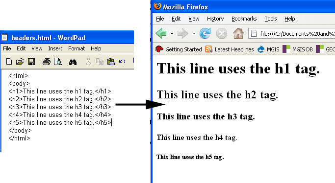
As the figure above shows, a web page can be authored using just a plain text editor. Most web pages (especially static ones) are saved with a .htm or .html file extension. When naming HTML files, it is best to avoid using spaces (use underscores instead) and punctuation.
Basic HTML Rules/Terminology
- The characters that denote an HTML tag (< and >) are referred to as angle brackets.
- Tags usually come in pairs (e.g., <body> and </body>, where <body> is the start tag and </body> is the end tag).
- HTML is not case sensitive (i.e., <title> is the same as <TITLE>), though lowercase is the recommended standard.
- Tags and their associated text form HTML elements.
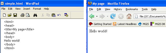
A simple HTML document
All HTML documents should be enclosed within <html></html> tags and should contain a head section and a body section. The head section contains metadata about the document and is defined using the <head> tag. The <title> tag is used frequently in the head section to define the title of the document. The body section contains the information you want to appear on the page itself and is defined using the <body> tag. Below is an example of a very basic HTML document:
Commonly used tags
As we saw earlier, the <h1>...<h6> tags are used to define headings. Other tags that are often used to define elements in the body of a document include:
- <p></p> to define paragraphs of text
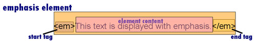
- <em></em> to give text emphasis (displayed in italics by default)
- <strong></strong> to give text strong emphasis (displayed in bold by default)
- <br> to insert a line break
- <hr> to insert a horizontal rule (line)
Note that a couple of these tags refer to the default presentation of their associated text. Later in the lesson, we'll see how stylesheets can be used to override these defaults.
Displaying lists
HTML allows authors to define two types of lists - ordered and unordered. Ordered lists are most appropriate when listing a set of steps or items that can be ranked in some way. The <ol> tag is used to begin an ordered list and the </ol> tag is used to end it. Within those tags, each item should be enclosed within <li> and </li> tags. By default, web browsers number the items automatically beginning with 1.
<html>
<body>
<h4>Ordered List</h4>
<ol>
    <li>Citizen Kane</li>
    <li>Casablanca</li>
    <li>The Godfather</li>
</ol>
</body>
</html>
|
 |
Unordered lists are most appropriate when listing items that cannot be ranked meaningfully. List items are defined the same way with <li></li>, but the items are enclosed by <ul></ul> rather than <ol></ol>. By default, web browsers mark the items with bullets.
<html>
<body>
<h4>Unordered List</h4>
<ul>
    <li>Ford</li>
    <li>GM</li>
    <li>Chrysler</li>
</ul>
</body>
</html>
|
 |
Note: The indentation of the list items in the examples above is done merely to improve the readability of the HTML code and is not responsible for the indentation of the items in the output. Writing the code such that the li elements appear flush with the left margin would result in the same output.
Displaying images
Images are added to a web page using the <img> tag. For example:
<img src="brown_MarkerA.png">
Some important points to note about this example:
- img elements don't have an end tag.
- src is an example of an element attribute.
- Attribute values should be specified in quotes, preferably double quotes.
- The web browser will look for brown_MarkerA.png in the same folder that the HTML document is in.
- It is also possible to load images using a full web address (URL):
<img src="http://www.personal.psu.edu/jed124/icons/brown_MarkerA.png">
Adding links
Links are added to a web page using the anchor tag (<a>) and its href attribute:
<a href="http://www.psu.edu/">Penn State</a>
Note that the text that you want to display as a link should be placed between the <a> and </a> tags. The URL that you want to load should be used to specify the href attribute value.
You've probably encountered pages with links that jump to other locations in the same page (e.g., a "Back to top" link). Creating this type of link is a two-step process:
- Create an anchor somewhere in the document: <a id="top"></a>
- Link to that anchor: <a href="#top">Back to top</a>
Note that the value assigned to the id attribute ("top" in this case) is entirely up to you. The key is to plug the same value into the href attribute and precede that value with a pound sign to specify that you're linking to an anchor in the same document.
HTML entities
Some of the characters you might want to display on your page require special coding because they have special meanings in HTML. For example, if you wanted to display an algebraic expression like x > 5, you'd need to use the code > since angle brackets are used to produce start and end tags.
Another aspect of HTML that can prompt the use of one of these entities is the fact that consecutive spaces in your HTML source code are treated as one. You can get around this by inserting one or more non-breaking spaces with the entity.
Some other commonly used entities include:
| Output char | HTML code |
|---|---|
| & | & |
| " | " |
| © | © |
| ÷ | ÷ |
| × | × |
HTML tables
Tables are commonly used in mapping mashups to display information associated with features on the map. A table is defined using the <table> and </table> tags. A row can be added to the table using the <tr> and </tr> tags. Individual cells of data can be added to a row using the <td> and </td> tags. Here is a very simple example:
<table> <tr> <td>Penn State</td> <td>Nittany Lions</td> </tr> <tr> <td>Ohio State</td> <td>Buckeyes</td> </tr> </table> |
 |
To add a border to a table, you set its border attribute to some whole number (of pixels):
<table border="1"> <tr> <td>Penn State</td> <td>Nittany Lions</td> </tr> <tr> <td>Ohio State</td> <td>Buckeyes</td> </tr> </table> |
 |
To include column headings, add a row containing <th> elements instead of <td> elements. By default, web browsers will display the <th> elements in bold:
<table border="1"> <tr> <th>School</th> <th>Mascot</th> </tr> <tr> <td>Penn State</td> <td>Nittany Lions</td> </tr> <tr> <td>Ohio State</td> <td>Buckeyes</td> </tr> </table> |
 |
<td> and <th> elements have an attribute called colspan that can be used to spread the element's text across multiple columns:
<table border="1"> <tr> <th colspan="2">2000</th> <th colspan="2">2006</th> </tr> <tr> <th>Males</th> <th>Females</th> <th>Males</th> <th>Females</th> </tr> <tr> <td>5,929,663</td> <td>6,351,391</td> <td>6,043,132</td> <td>6,397,489</td> </tr> </table> |
 |
Likewise, <td> and <th> elements also have a rowspan attribute for spreading text across multiple rows.
Miscellaneous notes
Comments can be inserted into an HTML document using the following syntax:
<!-- This is a comment. -->
Also, as mentioned above, consecutive spaces are ignored by web browsers. This means that you should feel free to indent your HTML code (as shown in the table examples) and use line spacing to make it easier to read and follow.
Online tutorials/cheatsheets
This section of the lesson is just an introduction to the basics of HTML. There are many other helpful online HTML tutorials that can help you learn the language, along with cheatsheets that can be used for quick reference once you've gained some coding experience. Here is a list of sites that I've found to be helpful:
XML/XHTML
What is XML?
HTML handles the needs of most web authors, but there are some kinds of information that it is not well suited for presenting (e.g., mathematical notations, chemical formulae, musical scores). The eXtensible Markup Language (XML) was developed to address this shortcoming. XML is a language used to define other languages, a meta-language. Just as HTML has its own syntax rules, you can create your own markup language with its own set of rules.
For example, here is an example of a markup language [17] used to store information about CDs in a CD catalog. Unlike HTML, in which the root element is called <html>, this language has a root element called <CATALOG>. A <CATALOG> element is composed of one or more <CD> elements. Each <CD> element in turn has a <TITLE>, <ARTIST>, <COUNTRY>, <COMPANY>, <PRICE>, and <YEAR>.
So, like HTML, XML documents use tags to define data elements. The difference is that you come up with the tag set. It is possible (though not required) to specify the rules of your XML language in a document type definition (DTD) file or an XML schema definition (XSD) file. For example, you might decide that a <CD> element can have one and only one <ARTIST> element within it.
While XML is quite similar in syntax to HTML (i.e., its use of tags), there are some syntax differences that make XML a bit more strict. Among these differences are:
- XML elements must have an end tag. Recall that the <img> element in HTML doesn't require an end tag.
- XML tags are case sensitive. <CATALOG> is not the same as <catalog> in XML, whereas <EM> is the same as <em> in HTML.
- XML elements must be nested properly. In HTML, an author can get away with code like <strong><em>Total</strong></em>, whereas in XML the </em> tag must come before the </strong> tag.
XML's Uses
XML has become an important format for the exchange of data across the Internet. And, as the CD catalog example discussed above implies, it can also be used as a means for storing data. We'll use XML later in the course for both of these purposes. Right now, we're going to focus on XML's use in creating a new flavor of HTML called XHTML.
An early development in the growth of web publishing was that desktop web browsers were designed to correct poorly written HTML. For example, in a bit of content containing paragraphs of text, it is possible to omit the </p> tag for paragraph elements and all of the popular desktop web browsers will render the content the same as if the </p> tags were present. This is not a surprising development if you think about it for a moment. Which browser would you prefer to use: one that displays a readable page the vast majority of the time or one that displays an error message when it encounters poorly written HTML?
Flash forward to the 2000s, the dawn of portable handheld devices like tablets and smart phones and wireless Internet. Slower data transfers and less computing power in these devices combined to produce lesser performance when rendering HTML content. This was one of the factors leading to the development of XHTML.
What is XHTML?
XHTML (eXtensible Hypertext Markup Language) is simply a version of HTML that follows the stricter syntax rules of XML. An XML/XHTML document that meets all of the syntax rules is said to be well formed. Well-formed documents can be interpreted more quickly than documents containing syntax errors that must be corrected.
The introduction of this new XHTML language came after years of the development of plain HTML content. Thus, web authors interested in creating well-formed XHTML had to adjust their practices a bit, both because of the sloppy habits that forgiving browsers had enabled and the outright differences with HTML. These adjustments include:
- Elements that don't require an end tag in HTML must have one in XHTML (e.g., <p> needs a matching </p>).
- Empty elements in HTML must be terminated in XHTML (e.g., <br> must be changed to <br></br> or its shortcut <br />).
- Elements must be properly nested.
<strong><em>Some text</strong></em> INCORRECT
<strong><em>Some text</em></strong> CORRECT - Attribute values must be quoted.
<table rows=3> INCORRECT
<table rows="3"> CORRECT - XHTML is case sensitive. <a> and <A> are different tags. The standard is to use lowercase.
Flavors of XHTML
HTML was originally developed such that the actual informational content of a document was mixed with presentational settings. For example, the <i> tag was used to tell the browser to display bits of text in italics and the <b> tag was used to produce bold text. An important aspect in the development of web publishing has been its push for the separation of content from presentation. This resulted in the creation of an <em> tag to define emphasized text and a <strong> tag to define strongly emphasized text. It turns out that the default behavior of browsers is to display text tagged with <em> in italics and text tagged with <strong> in bold, which may leave you wondering what purpose these new tags serve if they only replicate the behavior of <i> and <b>.
The answer lies in the use of Cascading Style Sheets (CSS). With CSS, web authors can override the browsers' default settings to display elements differently. Authors can also develop multiple style sheets for the same content (e.g., one for desktop browsers, one intended for printing, etc.). The usage of style sheets also makes it much easier to make sweeping changes to the look of a series of related pages. We'll talk more about CSS in the next section.
So, while it is possible to override the behavior of the <i> and <b> tags just as easily as any other tags, the <em> and <strong> tags were added and recommended over <i> and <b> to encourage web authors to move away from the practice of mixing content with presentation.
XHTML has two main dialects that differ from one another in terms of whether they allow the use of some presentational elements or not. As its name implies, the XHTML Strict dialect does not allow the usage of elements like <font> and <center>. It also does not allow the usage of element attributes like align and bgcolor. Presentation details like font size/type and alignment must be handled using CSS. The Strict dialect also requires that all text and images be embedded within either a <p> element or a <div> element (used to define divisions or sections of a document).
The XHTML Transitional dialect does not prohibit the use of presentational elements and attributes like those described in the previous paragraph. Generally speaking, XHTML Transitional was intended for developers who want to convert their old pages to a newer version, but would probably not bother to do it if they had to eliminate every presentational setting. XHTML Strict was intended for developers creating new pages.
XHTML developers specify which set of rules their page follows by adding a DOCTYPE line to the top of the page. For example, here are the DOCTYPE statements for XHTML Strict and XHTML Transitional, respectively:
<!DOCTYPE html PUBLIC "-//W3C//DTD XHTML 1.0 Strict//EN"
"http://www.w3.org/TR/xhtml1/DTD/xhtml1-strict.dtd">
OR
<!DOCTYPE html PUBLIC "-//W3C//DTD XHTML 1.0 Transitional//EN"
"http://www.w3.org/TR/xhtml1/DTD/xhtml1-transitional.dtd">
Browse this article for more details on the differences between the two dialects. [18]
The basic skeleton of an XHTML Strict document looks like this:
<!DOCTYPE html PUBLIC "-//W3C//DTD XHTML 1.0 Strict//EN"
    "http://www.w3.org/TR/xhtml1/DTD/xhtml1-strict.dtd">

    <html xmlns="http://www.w3.org/1999/xhtml">
        <head>
            <meta http-equiv="content-type"
                content="text/html; charset=utf-8"/>
            <title>Your title here</title>
        </head>
        <body>
            Your content here
        </body>
    </html>
Page validation and conversion
XHTML and its dialects were developed by a standards organization called the World Wide Web Consortium (W3C). They also provide tools for web authors [19] to validate that their pages follow the syntax rules of their selected DOCTYPE and to convert their pages from sloppy HTML to clean XHTML. This conversion tool is called HTML Tidy and can be run on the desktop or online (see links below).
HTML Tidy [20]
HTML Tidy (online version) [21]
Recent developments
Though XHTML was originally intended to be "the next step in the evolution of the Internet," it never gained a strong foothold in the web development community. A major factor that discouraged its adoption was that in order to reap the full benefit of an XML-based document, it needed to be served to browsers as "application/xhtml+xml" rather than "text/html." Most major browsers such as Firefox, Chrome and Safari were built to handle the "application/xhtml+xml" content type. The notable exception was Internet Explorer, which until version 9 did not support "application/xhtml+xml" content — users were asked if they wanted to save the file when documents of that type were encountered.
In addition to the content type issue, technological advances have undercut the argument that small handheld devices cannot load web pages at an acceptable speed without the use of an XML-based parser. Today's smartphone browsers utilize the same HTML parsers as their desktop counterparts.
Thus, in recent years, the notion of a world in which browsers parse all web pages as XML and page developers must author well-formed documents appears less and less likely. The W3C halted their development of a new version of XHTML and shifted their focus towards a new version of HTML (HTML5). This led some to declare that "XHTML is dead [22]." HTML5 requires browsers to continue correcting poorly written HTML. This has the effect of allowing sloppy page authors to continue in their sloppy habits. That said, browsers will continue to accept pages authored with XHTML-style coding, so developers who see value in serving their pages as XML may continue to do so. To learn more about HTML5 [23], see the short tutorial at the w3schools site.
So what language should we use?
HTML5 is the current standard for web publishing and you should certainly be looking to employ it in the web pages you develop. I have the content on XHTML in this lesson for a few reasons:
- to give you an appreciation for the evolution of web publishing standards,
- you're likely to encounter XHTML in other people's source code, and
- to encourage you to write clean HTML code. Doing so will enable you to achieve a higher level of consistency in the rendering of your pages than if you allowed yourself to pick up bad habits.
At the end of this lesson, you'll be asked to write a web page from scratch using what you learned from the lesson. I'm going to require you to write that page in XHTML Strict. However, for subsequent projects, you will be able to use the less rigid HTML5.
CSS
The need for CSS
During the early years of the World Wide Web, maintaining a site where all of the pages share the same style was tedious and inefficient. For example, if a web author wanted to change the background color of each page on his/her site, that would involve performing the same edit to each page.
Creating alternate versions of the same page (e.g., one for the visually impaired) was also frustrating since it involved maintaining multiple copies of the same content. Any time the content required modification, the same edits would need to be made in multiple files.
Also, the mixing of page content with its presentational settings resulted in bloated pages. This was problematic for a couple of important reasons:
- It decreased the readability of the HTML source code, for example when performing edits.
- It increased the page's file size, which in turn increased the time required to download it.
The Cascading Style Sheet (CSS) language was developed to address all of these issues. By storing presentational settings in a separate file that can be applied to any desired page, it is much easier to give multiple related pages the same look, to create multiple views of the same content and to reduce the bloating of pages.
How does CSS work?
To see how CSS works, go to this w3schools CSS demo [24]. Click on a few of the "Stylesheet" links beneath the Same Page Different Stylesheets heading and note how the same exact content is displayed in a different way through the use of different style sheets.
Next, click on the "Stylesheet1" link beneath the View Stylesheets heading to see the CSS code stored in that style sheet. The beginning of this stylesheet tells the browser to display text within the document's body element at 100% of the size set by the user (as opposed to shrinking or enlarging it) and in the Lucida Sans font. It also applies a 20-pixel margin and a line-height of 26 pixels. Scrolling down to the bottom of the stylesheet, note that the a element is set to display in black (#000000) and with an underline. If you scan through the rest of the document, you should notice some other useful settings. Don't worry if you don't follow all of the settings at this point; you should have a clearer understanding after working through this page of the lesson.
The basic syntax used in CSS coding is:
selector {property: value}
where selector is some element, property is one of its attributes and value is the value that you want to assign to the attribute. I'll again refer you to the w3schools site for more CSS syntax and selector [25] details. Pay particular attention to the "class selector," which is used when you don't want every element of a particular type to be styled in the same way (e.g., if you wanted some paragraphs to be aligned to the left and some to the right), and the "id selector," which is used to style a specific element.
Where to put CSS
CSS code can be written in three places:
- External style sheet - in an entirely separate file from the HTML document
- Internal style sheet - in the HTML document's head section
- Inline - the style is made an attribute of the desired HTML element
When the CSS code is stored in an external style sheet, a critical step is to add a reference to that style sheet in the HTML document's head section. The screen capture below (from the w3schools site) highlights this important setting.
To implement an internal style sheet, the actual CSS code should be stored in the head section of the HTML document rather than a link to an external file. The code should be surrounded by <style></style> tags as in this example:
  <style type="text/css">
    hr {color: sienna}
    p {margin-left: 20px}
    body {background-image: url("images/back40.gif")}
  </style>
</head>
Finally, to apply an inline style, the required CSS code should be assigned to the style attribute of the desired HTML element. Here is an example that changes the color and left margin settings for a paragraph element:
<p style="color: sienna; margin-left: 20px"> This is a paragraph </p>
Cascade order
The CSS language gets its name from the behavior exhibited when a page has styles applied from more than one of the sources described above. Styles are applied in the following order:
external — internal — inline
This order becomes important when the same selector appears in more than one style source. Consider the following example in which a page acquires styles from both an external and internal style sheet:
All h3 elements on the page will be colored red based on the setting found in the external sheet. The cascading nature of CSS comes into play with the text-align and font-size attributes. The page's h3 elements will take on the settings from the internal style sheet, since those styles were applied after the styles found in the external style sheet.
Now that you've seen how CSS works, the rest of this section will cover some of the more commonly used styles.
Background styles
The background color for any element (though most especially for the page's body) can be set as in the following example from w3schools:
<html>
    <head>

        <style type="text/css">
            body {background-color:yellow}
            h1 {background-color: #00ff00}
            h2 {background-color: transparent}
            p {background-color: rgb(250,0,255)}
        </style>

    </head>

    <body>

    	<h1>This is header 1</h1>
    	<h2>This is header 2</h2>
    	<p>This is a paragraph</p>

    </body>
</html>
|
 |
Note the different ways that the background-color property can be set. Valid values include names, 6-character hexadecimal values and RGB values. A list of valid color names can be found at w3schools. [26]
Text styles
The color of text can be altered using the color property. As with background colors, text colors can be specified using names, hexadecimal values or RGB values:
<html>
    <head>

        <style type="text/css">
            h1 {color: #00ff00}
            h2 {color: #dda0dd}
            p {color: rgb(0,0,255)}
        </style>

    </head>

    <body>

    	<h1>This is header 1</h1>
    	<h2>This is header 2</h2>
    	<p>This is a paragraph</p>

    </body>
</html>
|
 |
Text can be aligned to the left, right or center using the text-align property:
<html>
    <head>

        <style type="text/css">
            h1 {text-align: center}
            h2 {text-align: left}
            p {text-align: right}
        </style>

    </head>

    <body>

    	<h1>This is header 1</h1>
    	<h2>This is header 2</h2>
    	<p>This is a paragraph</p>

    </body>
</html>
|
 |
Underlining text and producing a strikethrough effect is accomplished using the text-decoration property. Note that this is also the property used to remove the underline that is placed beneath linked text by default. Removing this underline is sometimes desirable, particularly when lots of links are clustered near each other.
<html>
    <head>

        <style type="text/css">
            h1 {text-decoration: overline}
            h2 {text-decoration: line-through}
            h3 {text-decoration: underline}
            a {text-decoration: none}
        </style>

    </head>

    <body>

    	<h1>This is header 1</h1>
    	<h2>This is header 2</h2>
    	<h3>This is header 3</h3>
    	<p><a href="http://www.w3schools.com/default.asp">This is a link</a></p>

    </body>
</html>
|
 |
Recall from earlier that the font used to display the text of an element can be set using the font-family property and that it is a good idea to list multiple fonts in case the preferred one is not available on the user's machine.
Text can be sized using the font-size property. Note that valid values include percentages in relation to the parent element, lengths in pixel units and names like small, large, smaller, and larger.
<html>
    <head>

        <style type="text/css">
            h1 {font-size: 150%}
            h2 {font-size: 14px}
            p {font-size: small}
        </style>

    </head>

    <body>

    	<h1>This is header 1</h1>
    	<h2>This is header 2</h2>
    	<p>This is a paragraph</p>

    </body>
</html>
|
 |
To change the weight of text (i.e., its boldness), the font-weight property is used. Valid values include names like bold, bolder, lighter or multiples of 100 ranging from 100 to 900 with 400 being normal weight and 700 being bold.
<html>
    <head>

        <style type="text/css">
            p.normal {font-weight: normal}
            p.thick {font-weight: bold}
            p.thicker {font-weight: 900}
        </style>

    </head>

    <body>

    	<p class="normal">This is a paragraph</p>

    	<p class="thick">This is a paragraph</p>

    	<p class="thicker">This is a paragraph</p>

    </body>
</html>
|
 |
Margin styles
The space around elements can be specified using the margin-top, margin-right, margin-bottom, and margin-left attributes. These margin attributes can be set using values in pixel units, centimeters or as a percentage of the element's container. For example:
{margin-left: 2cm}
{margin-left: 20px}
{margin-left: 10%}
Note that all four margins can be set at once using the margin property. The values should be specified in the order top, right, bottom and left:
{margin: 2px 4px 2px 4px}
Table styles
Some of the more important styles to understand in a mashup context are those involving tables. The border properties are used to control the width, color and style (e.g., solid or dashed) of the borders of tables and their cells. Different settings can be applied to each side with separate declarations or the same settings applied to all sides in one declaration. The latter option, which is the most common, has this syntax:
border: thin solid gray
See w3schools' CSS Border page [27] for more details on the usage of the border properties.
Tables drawn with a border have their cells detached or separated from one another by default. Personally, I find this behavior to be annoying and prefer to collapse the borders using the setting:
border-collapse: collapse
 Table without a border-collapse setting (or set to border-collapse: separate) |
 Table with border-collapse: collapse setting |
Another default behavior that I find annoying is that empty cells are not displayed with a border. (This actually only applies to tables with detached borders; when borders are collapsed, empty cells will be visible no matter what.) To override this behavior, the empty-cells property is used:
empty-cells: show
Finally, the padding properties are used to specify the amount of space between the outside of an element's container and its content. Applying padding settings to td elements is commonly done to control the amount of space between a table cell border and its text. Again, padding can be controlled on a side-to-side basis or in a single declaration. The most common setting is to pad the cells equally on all four sides, which can be done as follows:
padding: 5px
The following CSS styling example [28] applies some of these styles and some that were described earlier to produce a visually appealing table:
CSStable {
background-color:#FFFFFF;
border: solid #000 3px;
width: 400px;
}
table td {
padding: 5px;
border: solid #000 1px;
}
.data {
color: #000000;
text-align: right;
background-color: #CCCCCC;
}
.toprow {
font-style: italic;
text-align: center;
background-color: #FFFFCC;
}
.leftcol {
font-weight: bold;
text-align: left;
width: 150px;
background-color: #CCCCCC;
}
|
HTML<table cellspacing="2">
<tr class="toprow">
<td> </td>
<td>John</td>
<td>Jane</td>
<td>Total</td>
</tr>
<tr>
<td class="leftcol">January</td>
<td class="data">123</td>
<td class="data">234</td>
<td class="data">357</td>
</tr>
<tr>
<td class="leftcol">February</td>
<td class="data">135</td>
<td class="data">246</td>
<td class="data">381</td>
</tr>
<tr>
<td class="leftcol">March</td>
<td class="data">257</td>
<td class="data">368</td>
<td class="data">625</td>
</tr>
<tr>
<td class="leftcol">Total</td>
<td class="data">515</td>
<td class="data">848</td>
<td class="data">1363</td>
</tr>
</table>
|
This code yields:
Assignment: Write a Page Using XHTML and CSS
You have been sent a Word document containing text that I’d like you to convert to a valid XHTML Strict document. Match the formatting found in the Word doc as closely as possible, paying particular attention to text alignment, font size and font weight. Some of the formatting will require CSS, which you should write in either an external file or in the head section of the XHTML doc.
The goal of this project is to test your ability to code the document from scratch, so avoid using applications that generate the HTML code for you such as Word. They almost invariably generate more code than is actually needed and your grade will be docked considerably if you use one. Instead, I recommend you use a basic text editor like Notepad.
You can refer to the links below for an example in which I've replicated a document similar to the one you've been assigned:
Example Word document [29]
My XHTML/CSS solution [30]
You may be tempted to find your assigned document online and copy its source code. To discourage this, I’ve made small modifications to each document. If I find that you’ve submitted a document that matches the original and not the one that I sent you, I will consider it an academic integrity violation (resulting in a grade of 0).
The addresses of links can be determined by right-clicking on one in Word and selecting Edit Hyperlink. The URL will be shown in the Address text box. You can highlight the complete URL using Ctrl-a and copy it to the Windows clipboard using Ctrl-c.
For full credit, your page must pass through the World Wide Web Consortium’s page validator [19] without errors.
Your e-Portfolio
From this point on in the course, you should be publishing your assignments to your PSU e-Portfolio (or to some other web host, if you prefer).
- Following the instructions in the Orientation [31], connect to your web space.
- There will be a default index.html page in your www folder. Modify this page (or create a new index.html page altogether) to include links to your first two assignments, along with anything else you want to include on your page.
- After uploading your index.html page, I will be able to view it through the URL http://www.personal.psu.edu/xyz123 [32], where xyz123 is replaced by your access account ID. (You should test this to confirm.) Note that when a URL ends in a folder name rather than a file name, the web browser looks for a file by the name of index.html or index.htm in that folder. This is why index.html can be omitted when attempting to view that page.
Deliverables
This project is two weeks in length. Please refer to the course Calendar, in Canvas, for the due date.
- Click on the Assignment 2 Submission link in Canvas to submit a link to your project page (a link to your e-portfolio index page is OK too, if it contains a link to your project). (70 of 100 points)
- I will be checking your page against the World Wide Web Consortium’s page validator [19]. For full credit, your page must pass through without errors. (20 of 100 points)
- Be sure to include a link to your app from Lesson 1 in your e-Portfolio (10 of 100 points).
- Complete the Lesson 2 quiz.
Summary and Final Tasks
In this lesson, you learned about the core languages involved in web publishing. While knowledge of these languages isn't completely necessary for producing maps with the Google Maps API, you are now likely to have a much better understanding of the pages in which your maps will reside and you'll also be better equipped to develop pages of a higher quality.
In Lesson 3, you'll be introduced to the Google Maps JavaScript API and use it to create a map of your hometown.
Lesson 3: Introduction to the Google Maps API
Overview
In Lesson 3, you'll be exposed to the "Hello, World" page of the Google Maps JavaScript API. Hello World programs [33] have been encountered by computer programming students learning a new language for many years. The folks who developed the GNU operating system have a funny list of Hello World programs [34] written by people of different ages and occupations. Perhaps you can find one that matches you.
To make sense of the Google Maps Hello, World page, you'll need to recall the web content authoring technologies covered in the previous lesson:
- Hypertext Markup Language (HTML)
- Cascading Style Sheets (CSS)
- HTML Document Object Model (DOM)
- JavaScript
After dissecting the various parts of the Google Maps Hello, World page, you'll finish the lesson by modifying the page to include a marker that depicts the location of your hometown.
Objectives
At the successful completion of this lesson, students should be able to:
- use the Google Maps website to locate places by various search methods;
- manually construct a URL that will load a desired Google Map;
- insert JavaScript into a web page;
- use JavaScript and the Google Maps API to add a custom map to a web page;
- set the initial extent parameters of a custom map;
- obtain information on how to work with objects defined in the API through the API Reference;
- add markers (points) to a map;
- cite examples of well-known Google Maps API apps.
Questions?
If you have any questions now or at any point during this week, please feel free to post them to the Lesson 3 Discussion Forum. (That forum can be accessed at any time by clicking on the Discussions tab within Canvas.)
Checklist
Lesson 3 is one week in length. (See the Calendar in Canvas for specific due dates.) To finish this lesson, you must complete the activities listed below. You may find it useful to print this page out first so that you can follow along with the directions.
| Step | Activity | Access/Directions |
|---|---|---|
| 1 | Work through Lesson 3. | You are in the Lesson 3 online content now. The Overview page is previous to this page, and you are on the Checklist page right now. |
| 2 | Complete "Plot Your Hometown" project. You will be working on this throughout the lesson.
|
Follow the directions throughout the lesson and on the "Plot Your Hometown" page. |
| 3 | Review a GIS mashup after you read the online content. | Find a Google Maps API mashup that catches your eye and write a short review of it in the Lesson 3 Discussion Forum. |
| 4 | Take Quiz 3 after you read the online content. | Go to the Canvas Homepage and click on the "Lesson 3 Quiz" link to begin the quiz. |
Introduction to Google Maps
Before we build our own Google Maps pages, we'll begin by taking a look at how Google's own mapping site works. Even if you've used this site before, you are likely to learn something from this section.
Please open a browser window to Google Maps [35] so that you can follow along with the discussion below.
Navigating the map
The user can pan the map to see what's just off the screen by clicking and dragging in the desired direction.
The user has multiple options for zooming in on the map, including double-clicking on the map in the area of interest, clicking on the plus sign in the lower right of the map (or minus sign to zoom out), or using the scroll wheel on the mouse (if available).
Also in the lower right corner of the map is a scale bar; clicking on it toggles between English and metric units.
In the lower left corner of the map is an icon that allows the user to switch between two primary map types: Map and Earth. The Map view displays a conventional reference map of political boundaries, place names, roads, railroads, water features, and landmarks. The Earth view displays satellite imagery or aerial photography, depending on the zoom level, with higher resolution data often available for major cities.
When in Earth view, a couple of additional controls appear above the zoom controls. The first enables rotating the view 90o, 180o or 270o. The red arrow will point north. The second control allows for applying two levels of tilt.
If you are a regular Google Maps user, you are probably aware that the search box at the top of the page can be used to locate places using full street addresses, just a city and state name, or even just a city name or zip code. However, it is also possible to locate places using airport codes (e.g., "LAX" for Los Angeles International) or latitude/longitude pairs (e.g., 40.8, -77.86 for Penn State's University Park campus). In addition, driving directions can be generated by separating any set of locations by the word "to" (e.g., "phl to state college, pa" to get directions from Philadelphia International Airport to State College). Businesses in close proximity to a location can be found by using the word "near" (e.g., "pizza near state college, pa") or by simply searching for a business type (e.g., "restaurants") when already zoomed in to the area of interest.
A collapsible control beneath the search box provides access to other background layer/overlay options. These include:
- Traffic - an overlay available in major cities that color codes highways based on the amount of congestion: red for heavy traffic, yellow for slow traffic, and green for normal-speed traffic
- Bicycling - routes originally obtained from the Rails-to-Trails Conservancy and augmented with user contributions
- Terrain - a layer that depicts the area using shaded relief
One last viewing option that warrants a mention is the Street View layer, which enables the user to view 360-degree panoramic photos taken at street level. Switching to Street View can be done by clicking on the "orange man" icon in the lower right and dropping him onto any blue line on the map. If the man icon is colored gray, then Street View is not available anywhere in the viewport.
Most of the site features discussed above are also available to third-party Google Maps developers. They can be arranged differently and unwanted controls can be left off the interface altogether. We'll come back to this later.
Inside Google Maps URLs
After searching for a location/business or generating driving directions, you can copy the URL in the browser's address bar to save it for later use, for example, to e-mail it to a friend. If you examine this URL closely, it has a number of parameters that will vary depending on the map type. Here is a simple Google map of State College [36] [https://www.google.com/maps/place/State+College,+PA/ [37]@40.7880144,-77.8525714,14z/data=!3m1!4b1!4m2!3m1!1s0x89cea899c13bdb73:0x9ce1c6c2833c8091].
Looking closely at this URL, here are some points to note:
- the spaces in "State College, PA" are replaced by + signs since spaces in URLs can create problems,
- the word "place" will be replaced by "search" or "directions" depending on the entry made in the search box (e.g., "coffee shops" or "philadelphia to harrisburg"),
- after the search term (in this case "State+College,+PA") comes the latitude/longitude at which the map should be centered (preceded by the @ symbol),
- after the map's center comes the zoom level ranging from 3z to 21z.
The URL often ends with a data parameter set to a long character string. Google has not made public how this string is constructed, though some bloggers have published some observations. It's a bit complicated, so I'll just point you toward the blog posts if you're interested in learning more:
New Google Maps URLs - Introduction from Sticklesville [38]
Stop Worrying About the New Google Maps; These URL Parameters Are Gold [39]
Knowledge of constructing URLs that can be parsed by the Google Maps servers has a lot of potential value. For example, if you had an Excel spreadsheet of addresses, you could generate a list of links that would open up a Google Map of each address. Excel's SUBSTITUTE function could be used to replace spaces in the addresses with + signs and the CONCATENATE function could be used to merge the address with the other required parts of the URL.
Now that you've gotten a brief tour of Google Maps, let's dive into creating your own custom mashup using the Google Maps API.
Orientation to the Google Maps API Reference
Google provides web developers with a number of APIs [40] (Application Programming Interfaces) for building geospatial applications. The most commonly used API (the JavaScript-based Maps API) is the one that we'll be learning about during this course. However, you should make a mental note of the other APIs that are available: two for developing native apps on mobile devices (one for Android phones and the other for iOS), and a set of location-based web services (e.g., the Elevation and Time Zone APIs).
The Google Maps JavaScript API home page [41] [https://developers.google.com/maps/documentation/javascript/] [42] is composed of 5 tabs:
- Overview: shows demos of the API's capabilities
- Guides: provides a high-level overview of various API concepts. This course will cover a lot of these same concepts, though you may find it worthwhile to use Google's Guide pages as a supplement to what you read here or to explore topics we don't cover.
- Reference: the place to go to obtain detailed information on the usage of the object classes built into the API.
- Samples: go here to find code examples in categories such as Basics, Controls, Drawing on the Map, etc.
- Support: provides a link to Stack Overflow's questions related to the Google Maps API and to a list of known API bugs
- Tutorials: self-explanatory
Now that we've seen where Google Maps developers go for information about the API, let's begin developing our own maps.
Building Your First Google Map Customization
The best way to build your first Google Map page is probably to use their "Hello, World" page as a starting point.
- Head over to the "Getting Started" section of the API documentation [43]. As the tutorial says, the first step in building a map page is to browse to the Google APIs Console to obtain an API key.
- Open the link to the Console page [44] in a new window or tab. We'll want to work with both the tutorial and console pages. If you don't yet have a Google account, sign up for one now. Then, log in to your account. You're likely to be asked how you can be contacted should you ever forget your password and to accept the terms of service. After going through all that, you should be looking at the Google Developers Console, with a Dashboard appearing in the primary window pane. The first thing we'll do is specify that we want to work with the Maps JavaScript API.
- Click on the Enable API link.
- In the list of APIs that appears on the right, click on Google Maps JavaScript API under the Google Maps APIs heading, then on the Enable button. Now we can move on to obtaining an API key.
- In the left-hand pane, click on the Credentials link.
- Select Create credentials > API key. You will be presented with a Create a new key dialog box.
- Select Browser key.
- In the text box beneath the Accept requests from these HTTP referrers... heading, enter the following:
*.personal.psu.edu/[your PSU access account ID]/*
For example, I entered *.personal.psu.edu/jed124/*
Note
It turns out that you don't really need an API key when working with the Maps API, but it's good to know how to obtain and use one in case you build a production application. If the API key gets in your way while testing (for example, when double-clicking your .html file on your local file system), you can remove the key. Just remove the text:
key=AIzaSyD1PO2RgLOjIXNSd3_OSQ_UTFJV4sQocBE (your actual key will differ). - Click Create to complete the creation of the key. We'll come back to the console page in a moment, so be sure to leave it open.
- Open Notepad or another plain text editor.
- Return to Google's Getting Started page, scroll down to the Hello, World section and copy and paste the code there into your text editor.
- Now go back to the Console page and copy your API key.
- In your text editor, locate the second script element and replace the API_KEY text with the key you just copied from the console page.
- Save the file as lesson3.html.
- Upload your lesson3.html file to your personal web space and confirm that you see a map of Sydney, Australia. (If you upload the file to your root web space, it will be available at the address http://www.personal.psu.edu/[your PSU access account ID]/lesson3.html.)
Now, unless you live in Sydney, this map probably won't be particularly useful to you. In the next section, we'll spend a good deal of time dissecting the various pieces of the code you just copied so that you are able to understand what each piece contributes to the page.
Dissecting the Google Maps Hello World Page
Let's examine this start-up page and discuss its various pieces. Now that you are familiar with HTML, you should recognize the <html>, <head> and <body> tags. You should also recognize that the <!DOCTYPE> directive declares that the document is written as HTML5.
After defining the page's title (Simple Map), the <head> of the document contains two <meta> elements. The first of these is concerned with rendering the document in a user-friendly way across a variety of devices (part of the larger CSS topic of responsive web design [45] [http://www.w3schools.com/css/css_rwd_viewport.asp]. [46] This is not critical for you to dive into now, but you may want to return to this topic if you are developing for mobile phones or tablets). The second meta element specifies that your document is encoded in the UTF-8 character set, one that supports all of the world's major languages. It's a good idea to include this line verbatim in all of your map pages. If you're an insomniac, you may want to read more about character encoding [47] [http://www.w3schools.com/charsets/default.asp] [48].
The next block of code within the head is a style element containing a few CSS settings. The basic idea behind these settings is to produce the best consistency in the rendering of the document by different browsers. The document as a whole (i.e., the html element) should take up 100% of the available space in the browser window. The body element, in turn, should take up 100% of its parent container, the html element. The body's margin and padding are also set to 0px, which in effect specifies that there should be no whitespace added to either the exterior or interior of the body element's boundary. Finally, the element with the ID of "map" has its height set to 100% of its parent container.
Next comes the body of the document, in which the first thing you'll find is a div element. div elements are used to create divisions, or sections, in a document. In a Google Maps API context, a div is typically used as the container for the page's map. Note that this div is assigned an id of map. This is consistent with the style setting mentioned a moment ago and, as we'll soon see, with the creation of the Map object in the JavaScript code.
After the map div, you'll find two <script> elements, which are used to define scripts written in JavaScript. The first of these elements specifies how to create the map to be inserted on the page (more on this later), while the second sets up a reference to the current version of the Google Maps API by setting the element's src attribute equal to a Google URL. Including this script element is critical to building a working application. Without it, the browser won't know what to make of the JavaScript code that's found in the first script element.
Learn More
At this point, you should familiarize yourself with the syntax of JavaScript (JS). The w3schools site offers a good hands-on JavaScript tutorial [49] that should do the job. Take a couple of hours to work through the topics listed under the JS Tutorial heading and pay particular attention to the following points:
- Ending statements with a semicolon is optional. (The start-up script from Google uses semicolons.)
- Note the difference between placing scripts inside the page's head section and its body section.
- JavaScript is a dynamically typed language; you do not need to specify a data type when declaring a variable.
- JavaScript variables are case sensitive.
- Variables can be initialized on the same line that they are declared.
- Code associated with a conditional statement (if or else statements) or a loop (for or while) must be enclosed in braces.
- Alert boxes can be used to debug scripts that aren't working properly.
- JS functions are reusable blocks of code with an optional return value.
- The backslash (\) can be used to insert special characters in a string (e.g., if you want a string enclosed in double quotes to also contain a double quote).
- Comments are signaled in JS using two slashes (//).
Now that you've learned a bit about JavaScript, we can examine the part of the file that loads the map onto the page. The first <script> element declares a variable called map, then defines a function called initMap(). Because the map variable is declared outside of the function, it has a global scope. In other words, if there were a second function -- say, loadData() -- the map variable could be used in that second function, whereas if the variable had been declared within initMap(), it would not be usable in a different function.
Before discussing what's going on in initMap(), first scan through it, and note the occurrence of the string "google.maps." This is an example of a namespace. The usage of namespaces is deserving of a lesson in itself, but you can get by with the basic knowledge that namespaces are used to prevent confusion when multiple classes share the same name. For example, the Hello, World page that we're discussing here references (or sources) a JavaScript code library stored on a Google server. One of the classes defined in that library is called Map. If you wanted to, you could develop your own class named Map, but you'd need a way to distinguish between your class and Google's. That's where namespaces come in. To use Google's Map class with no chance of confusion, we add the prefix "google.maps." to the class name.
To understand what's going on in initMap(), open the API Reference [50] in a new tab. The API Reference is a large page containing documentation on all of the entities built into the API. The Contents section at the top of the page (collapsed by default) provides links to the part of the page that deals with the associated entity (class, object specification or constant). For example, if you click on the Map class, you'll be redirected to the section that describes that class's constructor (i.e., information on the parameters that are specified when creating a Map object), its methods (actions that the Map class is programmed to perform), its properties (characteristics that uniquely define Map objects) and its events (interactions with the Map that are triggered by the user and can be programmed against by you the developer).
Method parameters (pieces of information the method uses in performing its action) are listed in parentheses after the name. If a parameter is optional, it will be listed with a question mark next to it. If a method returns a value when it is called, the type of return value will be listed next to the method name and parameters. Finally, there is a brief description listed for each method.
Note that some methods return a basic data type like a Number, String or Boolean, while others return an object (anything presented as a link). Following one of these object name links will jump you to that object's section of the documentation.
The API Reference is good for getting a sense of everything that you can do as a developer with the API. However, it is not always easy to translate the information found in the API Reference into a working custom map application. That is where the code Samples [51] page can be quite helpful.
Getting back to initMap(), it creates an object of the Map class, so we'll want to look at the constructor for that class. The documentation tells us that when creating a new Map object, we need to specify a container that will hold the Map. As we saw earlier, a div was created for this purpose and assigned an id of map. Getting a reference to that div element within your JavaScript code is done using the HTML Document Object Model (DOM).
Learn More
Once again, the w3schools site offers a good JavaScript HTML DOM tutorial [52]. This short tutorial should only take you 30-60 minutes to complete. Pay particular attention to the usage of the getElementById() and getElementsByTagName() methods.
Returning to the documentation of the Map class constructor, note that we can optionally specify a MapOptions object when creating a Map. Following the MapOptions link takes you to a section of the API Reference labeled "MapOptions object specification." The wording of this header indicates that we're dealing with a JavaScript object literal, a term that may seem intimidating, but is actually not too difficult to grasp. Object literals are basically a list of property/value pairs, in which the list is enclosed in curly braces and the property/value pairs are separated by commas. Unlike a class such as Map, an object literal has no class constructor, methods or events. In this case, the object literal is specified using two property/value pairs: a center property, which is itself set equal to an object literal defined as a lat/lng pair, and a zoom property, which is set to a value of 8. Note that it is possible to store an object literal in a variable. For example, an alternative to the syntax seen in the Hello, World script would look like this:
var myMapOptions = {
  center: {lat: -34.397, lng: 150.644},
  zoom: 8
}

map = new google.maps.Map(document.getElementById('map'), myMapOptions);
Finally, here are a couple of important points to note:
- The second script element uses two attributes to control the loading and execution of the Google Maps API code. The default behavior for browsers is to pause the rendering of other HTML elements when they encounter a script element. The async attribute (introduced in HTML5) tells the browser to continue rendering the HTML and to load and execute the JavaScript code at the same time. The defer attribute (which has been around longer than async) similarly tells the browser to continue rendering the HTML while it loads the JavaScript code. The difference with defer is that it instructs the browser to wait to execute the JavaScript until the HTML is fully rendered. The two attributes can be used together to still get the "don't-stop-rendering" behavior even in older browsers that don't support HTML5 (and async). You can find further discussion of these attributes in this blog post [53], if you're interested. I wouldn't be too concerned if you're a bit fuzzy on the topic though, as it's not critical for a novice developer to understand.
- What is critical to understand are the key and callback parameters appended to the API URL. If you're adapting this example to create a page of your own, you'll want to replace the "API_KEY" value with the one that you obtained earlier in the lesson. Likewise, the value assigned to the callback parameter (the name of the function to execute when the API is done loading) may need modification depending on how you name your initialization function. For example, if you name your function initialize rather than initMap, you'll need to change the callback parameter accordingly.
Now that you understand the workings of the Google Maps Hello, World page, you'll see how to add a marker to your map in the next section.
Adding Markers to a Google Map
The Google Maps API allows developers to add points, lines and polygons to the map as overlays. Point overlays are the most common and are represented in the API as Marker objects. We'll use the API Reference as a guide to adding a marker to our map.
- Open the API reference page [54] and search the page (Ctrl-F) for the Marker class.
Like many other classes in the API, the Marker class's listing in the API Reference includes a Constructor section. This indicates that an object of this class can be created using the new keyword followed by the class name (new google.maps.Marker). Inside the parentheses is a listing of the parameters that the developer must/can supply when creating the object. In the case of the Marker class, it has just one parameter called opts that is supplied using an object of the MarkerOptions class. The opts parameter has a ? beside it to indicate that it is an optional parameter. - Follow the MarkerOptions link to view its documentation.
Note that this class does not have a Constructor section in its documentation. This indicates that creating an object of this class involves using the object literal notation that we encountered earlier when we created a MapOptions object. Of the many properties listed beneath MapOptions, two are particularly important:- position: set using a LatLng object defining the point where you want the marker to appear, and
- map: set using a reference to the Map object on which the marker should be added.
- Follow the LatLng link to jump to its section.
The LatLng class constructor lists two required parameters (lat and lng). As implied by their names, these parameters are specified using numbers representing the desired point's latitude and longitude. The third, optional, parameter can be set to True to allow for lat/lng values outside -90/+90 and -180/+180.
So, with the information we've gathered from the API reference, we know that the steps for adding a marker to the map are to create a LatLng object, use that object to create a MarkerOptions object, then create a Marker object using the MarkerOptions object as an argument to the Marker class constructor. - Open your lesson3.html file in any text editor. We're going to add our marker in the same location that's being used for the map's center. Rather than specify the marker's position using an object literal as the Hello, World example specifies the map's center, let's create a LatLng object, store a reference to that object in a variable, then use the variable to set the marker's position.
-
Insert the following line to the end of the initMap() function:
var latlng = new google.maps.LatLng(-34.397, 150.644);
- Next, create a MarkerOptions object and set its position and map properties:
var myMarkerOptions = { position: latlng, map: map } - Finally, create the Marker and add it to the map:
var myMarker = new google.maps.Marker(myMarkerOptions);
- Save the page and test it in your web browser.
You may have noticed (and been confused) that latlng appears in the script as both the name of a variable and a class. The same goes for map. It's actually OK if this happens, but let's rename these variables to make the script a bit easier to follow. - Change the name of the variable that references the LatLng object from latlng to myLatLng. Note that changing this name requires updating the position property of the MarkerOptions object.
- Change the name of the variable that references the Map object from map to myMap. This requires updating the lines where the variable is declared, where it's initialized and where the map property of the MarkerOptions object is set. Here is the complete script if you'd like to confirm that you wrote it correctly:
var myMap;
function initMap() {
  myMap = new google.maps.Map(document.getElementById('map'), {
    center: {lat: -34.397, lng: 150.644},
    zoom: 8
  });

  var myLatLng = new google.maps.LatLng(-34.397, 150.644);

  var myMarkerOptions = {
    position: myLatLng,
    map: myMap
  }

  var myMarker = new google.maps.Marker(myMarkerOptions);
}
Going forward, you will not be expected to preface your variable names with "my" as we've done here. My rationale for doing it here is to help clarify what's a variable (changeable) and what's a property or class (not changeable).
Now that you've seen how to add a marker to a map, you're ready to modify your page so that it displays your hometown. If you see problems with the way the initMap() function was written above, that's good because I'll be expecting you to write the code more efficiently as part of your assignment. ![]()
Assignment: Plot Your Hometown
Given the large dose of conceptual material you were introduced to in this lesson, the project that you'll submit for grading will be rather short. Here are some instructions for completing the assignment.
If you completed GEOG 482 (or GEOG 160 for those on campus), you should have located the latitude/longitude coordinates of your hometown in Project 1 using the United States Geological Survey's Geographic Names Information System [55] or the Getty Thesaurus of Geographic Names [56] (for students outside the U.S.). If you have not taken that course, use those tools or any other resources at your disposal to find this information. (One handy way to get a location's coordinates is to pull it up in Google Maps, right-click on the location and select What's Here?)
Modify your lesson3.html page so that the map is centered on and a marker points to your hometown. The easiest approach to this problem would be to alter the two identical sets of coordinates left over from the lesson. However, I hope you'll recognize that repeating values in different parts of a program is generally a bad practice because of situations like this where you end up having to make revisions in multiple places. So, while you're changing the location displayed on the map, revise the code so that it is as efficient as possible.
Also, be sure that your page passes successfully through the W3C validator without errors. (You will probably receive 2 warnings, which are OK to ignore.)
Deliverables
This project is one week in length. Please refer to the course Calendar, in Canvas, for the due date.
- Post the map of your hometown to your e-portfolio. (60 of 100 points)
- Below the map, include some reflection on what you learned from the lesson and/or any concepts that you found to be confusing (minimum 200 words). (20 of 100 points)
- Find a map built using the Google Maps API that catches your eye, and write a short review of it in the Lesson 3 Discussion Forum. (20 of 100 points)
- Click on the Assignment 3 Submission link in Canvas to submit a link to your project page (a link to your e-portfolio index page is OK too, if it contains a link to your project).
- Complete the Lesson 3 quiz.
Summary and Final Tasks
In this lesson, you built your first Google Maps customization. Even the simple map that you created involves a number of different technologies (HTML, XML, XHTML, the HTML Document Object Model, and JavaScript) and it is important that you have a firm understanding of this material before moving on. If you skipped over the w3schools tutorials referenced in the lesson, be sure to go back and complete them.
In Lesson 4, you'll see how to spice up the rather dull product of Lesson 3 by adding navigation and map type controls, opening info windows when the user clicks on a marker, using a custom marker icon, and adding line and polygon overlays.
Lesson 4: Adding Basic Functionality to a Google Map
Overview
So far in the course, you've spent the bulk of your time learning about the various web technologies that are involved in the creation of even the simplest Google Maps page. The last project deliverable was quite basic, and you probably came away thinking that the map was a bit boring. In Lesson 4, we'll dig deeper into the API to learn how to produce a more useful and personalized map. At the conclusion of the lesson, you'll be asked to map a set of locations and enable callout windows to appear when those points are clicked.
Objectives
At the successful completion of this lesson, students should be able to:
- modify the default user interface (e.g., the map type controls and map navigation controls);
- add event handling code that produces custom behavior when certain events are triggered by the user (e.g., opening a callout window when a marker is clicked);
- display map markers using icons that have been created and published by others;
- understand the process involved in creating an icon image that can be used for displaying map markers;
- work with JavaScript arrays to add lines and polygons to a map;
- use GIS software to obtain the latitude/longitude coordinates of points to be displayed on a Google map.
Questions?
If you have any questions now or at any point during this week, please feel free to post them to the Lesson 4 Discussion Forum. (That forum can be accessed at any time by clicking on the Discussions tab within Canvas.)
Checklist
Lesson 4 is one week in length. (See the Calendar in Canvas for specific due dates.) To finish this lesson, you must complete the activities listed below. You may find it useful to print this page out first so that you can follow along with the directions.
| Step | Activity | Access/Directions |
|---|---|---|
| 1 | Work through Lesson 4. | You are in the Lesson 4 online content now. Click on the "Next Page" link to continue. |
| 2 | Complete the "Jen and Barry's" project on the last page of the lesson.
|
Follow the directions throughout the lesson and on the "Jen and Barry's" page. |
| 3 | Take Quiz 4 after you read the online content. | Go to the Canvas Homepage and click on the "Lesson 4 Quiz" link to begin the quiz. |
Modifying the Map's User Interface
In this lesson, you'll be adding to the code you wrote in Lesson 3, so create a copy of your lesson3.html file and call it lesson4.html.
Note
The code examples in this lesson and beyond do not utilize the "my" prefix on variable names that was suggested in the previous lesson. That naming scheme was only meant to clarify what were variables and what were object names from the API. Hopefully now you'll be comfortable with variables having the same name as the object classes they reference.
Unless otherwise specified, a Google map includes a set of controls in the upper-right corner that allows the user to switch between the available map types (Map, Satellite and Terrain). There is also a zoom control in the lower-right corner for zooming in/out on the map. Depending on the application or your personal preference, you may want to deviate from these defaults.
Modifying the default map type control
Altering the map type control involves creating an object of the MapTypeControlOptions [57] class. As with the MapOptions and MarkerOptions classes we encountered in Lesson 3, a MapTypeControlOptions object must be created as an object literal. It has a mapTypeIds property for specifying which map types should be made available, a position property for specifying where on the map the control should appear and a style property for specifying whether the control should be a set of side-by-side buttons or a drop-down menu.
In Lesson 3, we saw that the Hello World example initialized the map so that it displayed the basic road map using the ROADMAP map type ID. The other map type IDs currently built into the API are SATELLITE, HYBRID, and TERRAIN. These ID constants are accessed through the MapTypeId class, which like all classes in the Google Maps API, must be referenced through the "google.maps" namespace.
Setting the mapTypeIds property of the MapOptions object requires an array of MapTypeId constants. A simple way to produce an array in JavaScript is to enclose a comma-separated list of items in square brackets. Thus, the code for setting up a map to display only the Map and Hybrid options might look like this:
var mapTypeControlOpts = {
    mapTypeIds: [google.maps.MapTypeId.ROADMAP, google.maps.MapTypeId.HYBRID]
};
The ControlPosition class defines the constants that can be used to set the position of the map type control. These constants are TOP_LEFT, TOP_RIGHT, BOTTOM_LEFT, BOTTOM_RIGHT, TOP, BOTTOM, LEFT, and RIGHT. To position the map type control on the bottom of the map, you would use code like this:
var mapTypeControlOpts = {
    position: google.maps.ControlPosition.BOTTOM
};
Finally, the MapTypeControlStyle class defines the constants that can be used to set the style of the map type control. These constants are DEFAULT, DROPDOWN_MENU and HORIZONTAL_BAR. The HORIZONTAL_BAR style shows the map type options as a set of buttons arranged side by side horizontally and is best suited for maps viewed on a large display such as a desktop monitor. The DROPDOWN_MENU style lists the map type options in a hierarchical dropdown menu and is best suited for maps viewed on a small display such as a smartphone. The DEFAULT style enables the API to switch automatically between a horizontal bar and dropdown menu depending on the size of the browser window that's displaying the map rather than hard wiring one or the other. To display the map types as a menu (and use the same mapTypeIds and position settings from above), you would use code like this:
var mapTypeControlOpts = {
    mapTypeIds: [google.maps.MapTypeId.ROADMAP, google.maps.MapTypeId.HYBRID],
    position: google.maps.ControlPosition.BOTTOM,
    style: google.maps.MapTypeControlStyle.DROPDOWN_MENU
};
Once the MapTypeControlOptions object is defined, it can be used to set the mapTypeControlOptions property of the MapOptions class:
var mapOptions = {
    mapTypeControlOptions: mapTypeControlOpts
};
The MapOptions object would then be applied to the map as an argument to the Map class constructor, just as before.
This discussion presumes that you want to give users a choice of background layers. If you'd instead prefer to lock them into one map type, the MapOptions class has a Boolean mapTypeControl property that can be set to false to remove the map type buttons from the interface:
var mapOptions = {
    mapTypeControl: false
};
Modifying the map navigation controls
Past versions of the API made it possible for developers to select from a zoom control that included a slider and one that did not (i.e., just + and - buttons). The slider version of the control also included a set of four arrows for panning the map. At version 3.22, the option to implement the slider version of the control was removed. The zoom control is now a pair of + and - buttons, located in the bottom right of the map by default. The control can be re-positioned using one of the constants described above in the discussion of the map type control. For example:
var zoomControlOpts = {
    position: TOP_LEFT
};
Using the same mapOptions object literal from the previous section on customizing the map type control, you would use the zoomControlOpts variable to set the zoomControlOptions property.
var mapOptions = {
    zoomControlOptions = zoomControlOpts
};
The developer also has the ability to disable the zoom control altogether:
var mapOptions = {
    zoomControl: false
};
The elimination of the slider style of the zoom control also did away with the panning buttons. Users must pan the map by clicking and dragging (or by swiping on a touchscreen).
Modifying other map controls
Other map controls that can be customized by developers include the street view control and scale control. As with the ones discussed above, these controls can be enabled/disabled using the Boolean MapOptions properties streetViewControl and scaleControl. The street view control is enabled by default, while the scale control is disabled.
Besides enabling/disabling them, the only customization option available for these controls is the position of the street view control. The street view control ("pegman" icon) appears just above the navigation controls by default. Overriding this position requires creating a StreetViewControlOptions object much like the ControlOptions objects discussed above.
Summary
As you can see, the API provides developers with a fair bit of control over the user interface. One last point I want to bring to your attention is the disableDefaultUI property. If you want to build an interface that differs quite a lot from the default, you can set this property to true, effectively giving yourself a clean slate with which to work. Leaving the property unset means that any changes you make will have the default interface as the starting point.
The Google documentation devotes a full page to map controls [58] and I encourage you to consult that page for a more thorough discussion of this topic. You'll find a couple of working examples on this page along with information on adding your own custom controls.
Once you've experimented with the various controls discussed in this section and gotten a feel for modifying the user interface, move on to the next part of the lesson, where you'll see how to style the Google basemap.
Styling the Base Map
The Maps API provides a great deal of control over the appearance of the base map. The process of modifying part of the base map involves specifying a feature type (e.g., road, transit, water), an element type (e.g., geometry, labels) and the desired style for that feature/element. To illustrate these concepts further, let's have a look at the source code of a couple of examples. Note that these examples initialize the page slightly differently than the Hello World example discussed in the previous lesson. I recommend you consider Google's current Hello World initialization method a best practice, but you should also not be "thrown off" by the method used in the examples below. You're likely to see many slight variations like this if you look at other people's source code, such as in places like stackoverflow.
Example 1: Changing Colors
This first example produces a new map type (called "Styled Map") [59] in which the color of water and of state names has been altered. Let's look first at the creation of the styles variable. This variable is assigned an array of MapTypeStyle [60]objects -- in this case, two such objects. Note that each of these objects has three properties set: featureType, elementType, and stylers.
The featureType property is set using one of the MapTypeStyleFeatureType [61] constants: to 'water' for the first MapTypeStyle object and 'administrative.province' for the second.
The elementType property is set using one of the MapTypeStyleElementType [62] constants: to 'geometry.fill' for the first object and 'labels.text.fill' for the second.
Finally, the stylers' property is set using a MapTypeStyler [63]object. In both cases, this object has only its color property set, though other commonly set MapTypeStyler properties include visibility and weight.
With an array of MapTypeStyle objects created, the next step is to create a StyledMapType object. To create this object, the MapTypeStyle array is passed to its class constructor along with a StyledMapTypeOptions object literal composed of two property settings: map and name. The map property defines the Map object that the StyledMapType will be associated with, while the name property defines the label that will appear on the map type control.
The next step is to add the StyledMapType to the Map's MapTypeRegistry. That is done with the line:
map.mapTypes.set('styled', styledMapType);
styledMapType refers to the object created in the previous statement, while the string 'styled' is the name assigned to the map type in the registry. This name is entirely up to you, and you'll note that it's different in Google's example.
The next statement sets the map's opening map type to the 'styled' map type. In some contexts, you might omit this statement so that your styled map type is an option for the user to switch to, but is not the default.
A final important step is to add the StyledMapType to the map type control array. This is actually done near the beginning of the initialize() function when the mapTypeControlOptions property is set using the expression:
mapTypeIds: [google.maps.MapTypeId.ROADMAP, 'styled']
It may seem strange that this setting comes before the StyledMapType is actually created, but apparently it's OK to do this.
Example 2: Changing Feature Visibility
This second styled map example [64] demonstrates how you might go about simplifying what's shown on the base map by turning off a number of its features. As with the first example, the key to manipulating the components of the base map is to specify a feature type, element type and desired style.
The first featureType altered in this example is 'road'. Keep in mind that it is possible to manipulate different categories of roads (e.g., roads.highway, roads.arterial). The use of 'road' here indicates that the style setting should be applied to all types of roads.
The setting of the elementType to 'all' specifies that the style should be applied to both the geometry of the roads and their labels.
Unlike the previous example where we changed the colors of features, here we set the visibility of the road features to 'off'.
Continuing on through the script, note that a number of other base map features are turned off in a similar way (national boundaries, neighborhood boundaries, land parcel boundaries, points of interest, and transit features). Also note that locality features (showing urbanized areas) have not been turned off, but have been lightened by setting their lightness property to 40%.
This base map is similar to the light options that we saw in Google My Maps and ArcGIS Online in Lesson 1 and is especially appropriate in situations where you want to ensure that the user's attention is drawn to the map's overlays rather than features on the base map.
One final difference to note between this example and the previous one is in the application of the styles. In the previous example, a new map type was created and made available as an option for the user to switch to. In this case, the styles are applied across all the map types that are made available to the user -- in this case, ROADMAP and TERRAIN -- through the line:
map.setOptions({styles: visStyles});
Using the Styled Maps Wizard
To help API developers style their base maps, Google has put together a Styled Maps Wizard [65]. Let's walk through how you might use this wizard to reproduce the styling code we saw in Example 1 above.
- In the Selectors dialog, select Water under the Feature Type heading.
You should see the interface automatically scroll to the right to reveal an empty option list. This adjacent option list is empty because Google offers no sub-categories for the Water feature type. If you select any of the other main categories (such as Administrative), you'll see sub-categories. - Under the Element Type heading, select Geometry.
You should see the options Fill and Stroke appear to the right. (If you only see Stroke, be sure to scroll up though that list.) When dealing with polygon features as in this case, fill refers to the interior of the polygon, while stroke refers to its outline. Note: Experimenting with the wizard, it appears that no differentiation is made between the fill and stroke for many polygonal feature types (like Water). So don't be surprised if you are unable to assign separate colors for each of these. - Select Fill from the Geometry sub-options.
- Check the Color checkbox.
You should see the water features on your map change to gray since the RGB sliders initialize to the midpoint value of 128. Note that you can change the color by dragging the sliders, entering values between 0-256 or by entering a hexadecimal code.
With a color selected, note that the Map Style dialog on the right side of the window summarizes the selections you've made in the Selectors dialog. These selections are labeled under the heading Style 0. - Add a new style by clicking the Add button at the top of the Map Style dialog.
You should see a new entry in the Map Style dialog labeled Style 1 and that the options in the Selectors dialog have been reset. - Return to the Selectors dialog and make the following selections:
Feature type: Administrative > Province
Element type: Labels > Text > Fill
Color: Red = 255, Green = 128, Blue = 128
You should end up with red state labels like the ones in my Example 1, and again, a summary of your style settings in the Map Style dialog. - At the bottom of the Map Style dialog, click the Show JSON button to see the style settings in JavaScript Object Notation (JSON). If you were incorporating these settings into your own map, you could copy and paste this code from the JSON popup window into your web page.
Now that you've seen how you can style the Google basemap to your liking, let's move to the next page where you'll see how to display a callout window when a marker is clicked.
Handling Clicks on a Marker
A disappointing aspect of the map from Lesson 3 was that clicking on the marker didn't do anything. The behavior that you're probably used to seeing when a marker is clicked is that a callout window opens with some information about that marker. To add this kind of behavior, we need to add an event "listener" for our marker. This listener will enable us to execute a function whenever certain events are triggered with respect to the marker (e.g., when it is clicked, when it is double-clicked, or when the mouse moves over it). The full list of events supported by markers can be found by looking up the Marker class in the API Reference. We will add a handler for the click event that will open an info window and display text that we've encoded as HTML.
Like several other classes we've encountered so far, an object of the InfoWindow class can be created by passing an "Options" object to its class constructor. So we'll start by defining an InfoWindowOptions object using object literal notation.
-
Add the following code (in which the long URL has been split across two lines for readability) to the end of the initMap() function:
var infoWindowOpts = {
  content: '<a href="https://www.youtube.com/watch?v=aLSFcF8SOiw">' +
    'My Hometown</a>'
};

var infoWindow = new google.maps.InfoWindow(infoWindowOpts);
The first statement in this block of code (which spans four lines) creates an object literal and sets its content property equal to a string of HTML that we want to display in the info window - a link to a website. Pay close attention to the two pairs of quotes used in this statement. The first pair is a set of single quotes used to enclose the entire string that is to be assigned to the content property. The second pair is a set of double quotes used to enclose the URL that's being assigned to the href attribute of the anchor tag. It would also be acceptable to use double quotes around the full string and single quotes around the URL. The important thing is that one kind of quotes be used to set the JavaScript content property and the other kind be used to set the HTML href attribute.
The second statement creates an InfoWindow object based on the content setting defined in infoWindowOpts. We're now ready to create the event listener.
-
Add the following code where you left off:
google.maps.event.addListener(marker, 'click', function() {
  infoWindow.open(map, marker);
});
This code calls the addListener() method in the event namespace, passing it the object whose events we want to listen for (marker), the event we want to listen for (click), and a function to execute when that event is triggered.
Even if you're an experienced programmer, the code used for the third argument may have you scratching your head a bit. We could have supplied the name of a function that was defined elsewhere in the document, but instead we're using something called an anonymous function. Anonymous (or inline) functions have a number of uses in JavaScript that are beyond the scope of this class, so we won't discuss them in depth. For our purposes, you should simply understand that they are frequently used to define the code to be executed as part of an event listener. Note that the function is defined in the same way as a normal function, with the exception that it is left unnamed.
In this case the anonymous function is just one line in length, calling on the open() method of the InfoWindow. The open() method's first parameter specifies the Map to display the InfoWindow on, while the second specifies an object to anchor the InfoWindow to (typically a Marker, Polyline or Polygon).
-
Save the file and reload it in your browser. Clicking on the marker should now open an info window that contains a link to a website. Note that we could have inserted any amount of HTML text into the info window.
Now, let's say we want to add a second marker with its own associated info window text. We could repeat the same statements (beginning with the creation of the latlng variable and ending with the call to the addListener method). I've added such code to an example page so that you can see why an approach like this doesn't work:
Note
Do not enter this code into your file. This is the wrong way to add a second marker. We'll see a better way to do this momentarily.
var latlng = new google.maps.LatLng(40.812, -77.8565); var markerOpts = { position: latlng, map: map }; var marker = new google.maps.Marker(markerOpts); var infoWindowOpts = { content: '<a href="http://www.gopsusports.com/facilities/' + 'beaver-stadium.html">Beaver Stadium</a>' }; var infoWindow = new google.maps.InfoWindow(infoWindowOpts); google.maps.event.addListener(marker, 'click', function() { infoWindow.open(map, marker); }); -
View my bad marker example page [66] and click on the markers to see why there is a problem with adding a second marker this way. If you click on the northern marker, an info window opens with the correct text. However, if you click on the southern marker, the info window associated with the northern marker opens again.
Note that this piece of code re-uses a number of variables that I had defined earlier in the script. The problem with re-using these variables in this way is that when the click event for either marker is being triggered, the variables are holding the values last assigned to them, rather than the values that were originally assigned when the event handlers were set up.
The simplest solution to this problem is to use different variable names for each marker (e.g., infoWindowOpts2, infoWindow2). However, if you're adding more than two or three markers, you'll find that such a solution is inefficient. A better solution is to create a function you can call on any time you want to create a new marker with an associated info window. That is the approach we'll take.
-
Add the following function to your lesson4.html file, just prior to the initMap() function (after the initMap() function would be fine also):
function createMarker(point,info,map) {
  var markerOpts = {
    position: point,
    map: map
  };

  var marker = new google.maps.Marker(markerOpts);

  var infoWindowOpts = { content: info };
  var infoWindow = new google.maps.InfoWindow(infoWindowOpts);

  google.maps.event.addListener(marker, 'click', function() {
    infoWindow.open(map,marker);
  });
}
This function accepts a LatLng object for its first parameter (stored locally in the function in the point variable), a string for its second parameter (stored in the info variable) and a Map object for its third parameter. A marker is created from the point and a handler is set up for the marker's click event that displays an info window containing the text passed into the info variable. The marker is added to the Map object passed into the map variable. (It might help to keep in mind that pages aren't restricted to having just a single map.)
In the next few steps, we'll modify the initMap() script so that it creates the marker using the new function.
First, a word about the map variable. Going back to the Google Hello World example, you've been working with a map variable defined outside your initMap() function. This gives the variable a global scope, meaning it can be used in any script or function found in the document. Thus, in this new createMarker() function we just added, we could easily utilize the global map variable to specify which map the marker should be added to. If we were going that route, it would not make sense to define a map parameter in the createMarker() function definition. However, defining the function with a map parameter makes it a bit more flexible because it won't be locked into adding markers to a single map. When going this route, it doesn't make sense to use a global variable for the map. -
Remove the var map statement found outside your initMap() and createMarker() functions.
- Back in the initMap() function, insert the var keyword at the beginning of the line that defines the map variable. This gives it a scope local to the initMap() function.
- Remove the var infoWindowOpts, var infoWindow and addListener() statements.
-
Modify the var marker statement to read:
createMarker(latlng, '<a href="https://www.youtube.com/watch?v=aLSFcF8SOiw">' +
  'My Hometown</a>', map);
- Next, add code for a second marker. You can simply modify the lat/long coordinates you used for your first marker slightly if you can't think of a good place to put the second one. You may need to change the initial zoom level of the map to see both markers. Re-use the same latlng variable that you used for the first marker. After adding the code, your page's source should look something like the source of this good marker example page [67].
- Test your page to confirm that it behaves as expected. This version of the code doesn't suffer from the error we encountered above - even though it also re-uses the same variable names - because embedding the anonymous function inside the createMarker() function creates something referred to as a function closure. Each time the createMarker() function is called, new copies of its local variables are created and the values held by the variables in previous calls to the function are retained separately. Thus, each Marker object created by the createMarker() function carries with it its own properties. A complete understanding of how function closures work is beyond the scope of this course, so don't worry if you're confused. You won't be asked about them on the quiz. :-)
Now that you've seen how to display an info window in response to a click on a marker, let's see how you can plot a marker using a custom icon.
Changing the Marker Icon
Unless you specify otherwise, markers you add to a map will be displayed using a red teardrop-shaped icon with a black circle at its center. However, you can change this icon to any image stored in .png format that has been sized appropriately. We'll first look at some icons published by fellow Google Maps developers. Later, we'll see how you might go about creating your own icons.
Using existing icons
There are lots of sites that provide useful Google Maps icons. Here are some of my favorites:
- Map Icons Collection [68] - a large number of categorized icons whose colors can be customized
- Benjaminkeen.com (Google Maps: Colored Markers) [69] - icons lettered from A-Z in ten different hues
- Marker Icons (from Portland State University) [70] - numbered icons in different hues
- In your web space, create an icons sub-folder within your geog863 folder.
- Go to Benjamin Keen's site and download his zip file of icons in .png format.
- Choose a color and upload the images labeled A and B to your icons folder.
We saw earlier that Marker objects can be created by passing a MarkerOptions object to their class constructor. And we saw that when defining the MarkerOptions object, you must set the map property to specify which Map object the Marker will be added to and the position property to specify where on the Map to place the Marker. When assigning a custom icon to a Marker, there are two optional properties that you may want to set: icon and shape.
We'll begin with the icon property as it's the most important. This property is set by specifying an Icon as an object literal. This object allows you to specify the URL of the image, its size, what part of the image you want to contact the map, and whether the image is being scaled down from a larger size.
Because the Icon object is required when we create the Marker, we're going to add the Icon code to the createMarker() function. Our first step will be to modify the function's input parameters to include a variable that will hold the name of the desired icon. -
Return to your lesson4.html document and add a variable named img to the createMarker() function's parameter list after the map variable:
function createMarker(point,info,map,img) { -
Next, above the code that already exists inside the function, specify an Icon object as follows:
var iconURL = 'icons/' + img;
var iconSize = new google.maps.Size(20,34);
var iconOrigin = new google.maps.Point(0,0);
var iconAnchor = new google.maps.Point(10,34);

var myIcon = {
  url: iconURL,
  size: iconSize,
  origin: iconOrigin,
  anchor: iconAnchor
};
The first line of this code creates a string defining the location of the icon image. In this case, the image is located in a sub-folder -- relative to the location of the HTML page -- named icons, so the URL is built by concatenating 'icons/' with the name of the image that was passed into the createMarker() function.
The next line creates an object of the Size class and stores a reference to it in a variable. Size objects are defined simply by specifying their width and height in pixels within the class constructor.
The next two lines create objects of the Point class, a class that is used to create objects that define positions on images in pixel coordinates. For example, the coordinates defining the center of a 16x16 pixel image would be 8,8. When defining a Point object, the first argument to the class constructor is the x coordinate and the second argument is the y coordinate. Here the first Point object is being used to define the coordinates of the image's origin (the pixel in the upper-left corner). It is generally a good idea to set these coordinates to 0,0. The second Point object is being used to define the part of the image that should appear to be touching the map (i.e., where it should be anchored). For the teardrop-shaped icons, the anchor point should be defined as 10,34 (10 pixels to the right of the origin and 34 pixels down). It turns out that the API assumes an anchor point of (width/2, height) if one is not defined, so it is not really necessary to define one for this icon. But this shows you how to define the anchor point if you use an icon that has a different shape.
Note
You can find the width and height of an image in Windows Explorer by right-clicking on it, selecting Properties, and viewing the Details tab. You can determine the coordinates of your image's anchor point using any image manipulation software. For example, in Microsoft Paint, you would simply open the image, hover the mouse over the desired anchor point and make note of the coordinates reported in the lower right of the window.
Finally, the four variables are used to set the properties associated with Icon objects. These property settings are stored in a variable called myIcon. With the Icon created, it can be used to set the icon property of the MarkerOptions object.
-
Add the line in bold to your code:
var myMarkerOpts = {
  position: latlng,
  map: map,
  icon: myIcon
}
Recall that we added an img parameter to the createMarker() function's parameter list. Our next step will be to return to the initialize() function and specify the desired image name when making a call to the createMarker() function.
-
In the initialize() function, modify the calls to the createMarker() function so that they include the name of the desired icon (I used blue, you should specify the color you uploaded to your web space):
createMarker(latlng,"some info window content",map,"blue_MarkerA.png");
...
createMarker(latlng,"some other info window content",map,"blue_MarkerB.png");
Note
There are a number of different ways to set up the passing of the icon name to the createMarker() function. For example, if your page only used blue markers, you could choose to "hard-code" that into the function (var iconURL = 'icons/blue_Marker' + img + '.png';). In that scenario, your calls to the function would simply include the desired letter ('A', 'B', etc.).
When using someone else's images as we did here, be sure that the owner of the images does not object. Also, save a local copy of the images to your server instead of referencing the originals. It is bad etiquette to ask someone else's server to serve icons that are being used on your site.
At this point, you could view the map and see your custom icon. However, the map would suffer from a relatively minor deficiency: when hovering the mouse cursor over the icons, the cursor will change (i.e. the marker will become clickable) whenever the cursor is hovered over the entire 20x34 image instead of just the visible part of the image. To fix this problem, we'll need to set the MarkerOptions object's shape property.
The shape property is set using a MarkerShape object, which has two required properties: coord and type. See the documentation of the MarkerShape class [71] and note the different ways of specifying the shape depending on whether the marker is circular, rectangular, or irregular. In this instance, our marker has an irregular shape, so we need to set the type property to 'poly'. We also need to set the coord property equal to an array of x/y coordinate pairs that delineates the shape. - Add the following code to create the MarkerShape object:
var iconShape = [8,33, 6,21, 1,13, 1,5, 5,1, 13,1, 18,6, 18,13, 12,21, 10,33];
var myMarkerShape = {
  coord: iconShape,
  type: 'poly'
};
Note that I inserted spaces between coordinate pairs to make the list more readable. The spaces make no difference to the API.
To determine the coordinates that describe your marker's shape, you should use some sort of image manipulation package like MS-Paint. Trace the boundary of the icon with your mouse, stopping where you would place the vertices if you were digitizing the shape in GIS software, for example. The software should report the coordinates as you move the mouse around, so you should jot down the coordinates at each stop.
-
Finally, we can set the shape property of the MarkerOptions object by adding the code in bold:
var myMarkerOpts = { position: latlng, map: map, icon: myIcon, shape: myMarkerShape } - Save your document, re-load it in your browser and confirm that it looks and behaves as expected.
Creating your own icons
As mentioned above, any png-formatted image can be used as an icon for markers you add to your maps. If you wish to create your own icon, here are a number of points to consider:
- You will want to make sure the icon is sized roughly the same as Google's default icon (20 pixels wide by 34 pixels high) or smaller. It need not have the same exact dimensions, but you should avoid using images that have more than 40 pixels in either dimension.
- You may need to add a leader line to the image, so that the image's anchor point is clear to the user.
- The handy site FavIcons From Pics [72] offers an easy way to create a .png file from other image formats such as .jpg or .gif. The site's primary purpose is to create .ico files that can be used to display a small logo to the left of the URL in a browser's address bar, but part of the zip file output is a .png file that happens to be a good size for mashup icons.
Now that you've seen how to jazz up your pages a bit with custom marker icons, let's move beyond plotting simple points to more complex line and polygon geometry.
Adding Lines and Polygons
Though you won't be expected to create maps with lines or polygons at this stage in the course, we're going to cover how to do so now. You can copy and paste the example code into test documents of your own if you like, but it is also OK if you just read through the examples.
Adding Lines
Adding a line to a map actually involves creating an object of the Polyline [73]class. The name Polyline comes from the fact that a number of shorter straight lines are drawn in sequence to build the complete geometry. A straight line is drawn between the first vertex and the second vertex. Then another straight line is drawn between the second vertex and the third vertex. This continues until the last vertex in the sequence is encountered and the polyline is complete.
As you might guess, a Polyline is created by passing a PolylineOptions [74]object to the Polyline class constructor. As with the MarkerOptions class, a PolylineOptions object must have its map property set to specify which Map the Polyline should be added to. However, unlike MarkerOptions which has a position property that is set using a LatLng, PolylineOptions has a path property that is set using an array of LatLng objects.
To customize the look of the Polyline, the PolylineOptions class has three simple properties:
- strokeColor - set using a hexadecimal color value, just like those we encountered in the Lesson 2 content on CSS,
- strokeOpacity - set using a value from 0 to 1 depending on the extent to which you want the user to be able to see the base map behind the line; 0 produces a fully transparent line and 1 a fully opaque line, and
- strokeWeight - set to the desired width in pixels; values in the range 1-4 are typical.
Here is a simple example of a three-vertex line drawn in red with 100% opacity and four pixels in width:
var lineCoords = [
   new google.maps.LatLng(40.73033, -77.87844),
   new google.maps.LatLng(40.812, -77.8565),
   new google.maps.LatLng(40.812419, -77.922449)
];

var lineOpts = {
   path: lineCoords,
   map: map,
   strokeColor: "#FF0000",
   strokeOpacity: 1.0,
   strokeWeight: 4
};

var line = new google.maps.Polyline(lineOpts);
The first statement creates the array of LatLng objects representing the desired line. Recall from earlier in the lesson that a simple way to construct an array is to put together a list of items separated by commas and enclosed within square brackets. In the next lesson, we'll dig deeper into other ways arrays can be constructed.
After the array is built and stored in the lineCoords variable, the next statement creates a PolylineOptions object as an object literal. The lineCoords array is used to set the path property, a variable called map is used to set the map property, the hexadecimal value of "#FF00000" is used to set the strokeColor to red and the strokeOpacity and strokeWeight properties are set to the values of 1 and 4 respectively. A variable called lineOpts is used to store a reference to the PolylineOptions object literal.
With the PolylineOptions object defined, the last statement passes that object to the Polyline class constructor to create a new Polyline object.
You can see this code in a complete working example (polyline) [75].
Adding great-circle lines
By default, the lines connecting the vertices in a Polyline are drawn such that they are straight in the two-dimensional Mercator projection used by the base map. But the Earth is not flat and the default two-dimensional lines are not really the shortest paths between the points. Great-circle lines (also called geodesics) represent the true shortest paths because they take the Earth's curvature into account. For large-scale maps like the one above, the difference between three-dimensional paths and two-dimensional paths is negligible, and you as the map author need not worry about the issue. However, if your map is of a regional or continental scale, the difference may be quite significant.
Fortunately, switching from a two-dimensional polyline to a geodesic is as simple as setting the PolylineOptions object's geodesic property to true. Have a look at this geodesic example [76] showing both types of lines connecting Miami to San Francisco.
In addition to illustrating the geodesic concept, this example also shows how properties of an object literal can be re-set to new values after they've been initialized. Because I wanted to draw the same Polyline with different values for just the geodesic and strokeColor properties, I didn't need to create a new PolylineOptions object. I could simply refer to the existing object through the lineOpts variable name and use the 'object.property = value'' syntax to assign new values to the properties I wanted to change.
Adding Polygons
Adding simple polygons to a map follows a pattern similar to what you just saw for lines. The end goal is to create a Polygon [77]object from a PolygonOptions [78]object. As with Polylines, you need to create an array of LatLng objects that delineate your Polygon's boundary. (I recommend making the last LatLng in the array the same as the first, though the documentation says that Polygons will close themselves if not closed explicitly.) Like PolylineOptions, PolygonOptions objects have a strokeColor, strokeOpacity, and strokeWeight property. These properties control the appearance of the polygon outline. To control the appearance of the polygon's interior, you will need to set the fillColor and fillOpacity properties.
Have a look at this PolygonsOptions example [79] showing the boundaries of the District of Columbia. Note in the source code that the fillColor and fillOpacity are not set. This demonstrates that the default values for these properties appear to be gray and ~50% opaque.
You should also note from the example that PolygonOptions doesn't have a path property, but instead a paths property. This difference arises from the fact that the API also allows for the display of more complex polygons, such as those with holes in their interior (donut polygons) and those made up of multiple parts (like the islands of Hawaii). In both cases, the idea is to create an array of coordinate arrays. In other words, for a donut polygon, you would create one coordinate array depicting the exterior of the polygon and a separate array depicting the hole. For a multi-part polygon, you would create a separate array for each part. Once all the coordinate arrays have been stored in variables, those coordinate array variables should be put into an array and used to set the paths property. This example demonstrates the depiction of a famous donut polygon, the Pentagon. [80]
Coding Tips
So far in the course, you've been encouraged to use a plain text editor like Notepad and have received little guidance on the topic of debugging code that's not producing the desired result. There are a number of tools out there that can make your job as a developer easier, and that will be the focus of this part of the lesson.
jsFiddle
jsFiddle.net [81] is a "playground" environment for seeing code and its output side-by-side. HTML, CSS and JavaScript code is entered in separate boxes, then the output is shown in a fourth box. Here's a quick tutorial on using jsFiddle:
- Go to this fiddle [82] to see Google's Hello World example.
- Edit the code in some way (e.g., change the map's center coordinates), then click the Run button. You should see your desired changes reflected in the Result window.
- Note the steps I took to adapt the Hello World code to jsFiddle:
- I entered only the HTML elements found in the body of the document.
- I removed the key parameter from the script element that references the Maps API.
- I omitted the style tags and script tags that would otherwise be found surrounding the code in the CSS and JavaScript boxes, respectively.
- I changed the selection in the second dropdown list under Frameworks & Extensions from onLoad to No wrap - in <body>. This specifies that you want the code in the JavaScript box to be executed as if it was in the body of the HTML document.
jsFiddle is often used by the folks who participate in help forums such as Stack Overflow. If you find yourself in need of help down the road, putting your code into jsFiddle and including a link to your fiddle in your post would be a good idea.
Note: Google used to maintain a similar environment specifically for their APIs called the Google Code Playground. That no longer appears to exist, but I encourage you to keep your eyes open to see if they resurrect it.
Development Environments
Plain text editors like Notepad are OK for beginners getting to know web-publishing languages, but there are more advanced tools out there that make the developer's job easier. Integrated Development Environments (IDEs) are software applications that allow developers to write, test, and debug source code all in one application. IDEs also typically provide auto-completion and syntax highlighting. Examples of popular IDEs include Microsoft Visual Studio and Eclipse. Google's Code Playground can be thought of an online JavaScript IDE. However, it lacks syntax highlighting and, obviously, does not allow for editing code stored on your local file system.
There are lots of IDEs suited for web development, as a web search for "web development ide" [83] will show you. For the purpose of continuing on through this course, I'm going to recommend Notepad ++ [84]. As its name implies, It's a step (or two) up from Notepad. My main reasons for pointing you to it are that it is free, it's easy to use, and it provides line numbers and syntax highlighting. Notepad++ is arguably not a true IDE since it's not possible to view your pages directly within the same application, but it does allow you to easily launch them in various web browsers, so I think it's a rather pointless debate.
Let's walk through a short set of steps to familiarize you with Notepad++.
- Download and install Notepad++. [85]
- Open your lesson3.html page in Notepad++. An easy way to do this is to browse to it through your file system, right-click on it, and select Edit with Notepad++.
The first thing you should notice is the formatting applied to your code. HTML elements are shown in blue, attributes in red, and attribute values in purple. This happens because your file has a .html extension. Keep in mind that if you create a new page from scratch, you will not see this highlighting done until you save it with a .htm or .html extension.
Next, note the boxes just to the left of several lines in your code. These boxes appear at the beginning of blocks of code that can be logically treated as a unit. - Click on the box next to the style element in the head of the document to collapse that code. The minus that had been inside the box will have changed to a plus, indicating that clicking it again will re-expand that code unit.
- Move your cursor down through the document until you reach the first script element (the one that sources the Maps API). You should see that the first and last lines of that element are highlighted. This highlighting can be very helpful, especially if you haven't done a good job of indenting your code logically.
- Continue moving the cursor down the document until you reach the line that defines the var mapOpts variable. Move the cursor to the right until you reach the opening brace. You should see that the brace is highlighted and a red line appears connecting the opening brace to its matching closing brace. The same behavior can be observed with brackets and parentheses. Given how often these characters are used in JavaScript -- and the importance of ordering them correctly -- this feature can be quite useful.
Now that we've worked with a more fully-featured source code editor, let's discuss some tips for working out the kinks in pages that aren't giving you the results you expect.
Debugging
So, what do you do when you load your page in a browser and get... nothing? Thankfully, there are tools that can help pinpoint problems in your code without having to manually search line by line. Let's have a look at a couple of broken Hello, World pages and how we can determine why they're broken.
- Load the first Hello World example [86] in IE, Firefox, or Chrome. Your browser window should be blank because of an error in the page.
- Open the JavaScript console as follows:
Chrome - click on the menu icon (3 stacked lines to the right of the address bar), then select More Tools > Developer Tools > Console.
Firefox - click on the menu icon and select Developer > Web Console.
IE - 1. From the Tools menu, select F12 developer tools (or simply hit the F12 key). 2. Click on the Console tab. 3. Reload the page.
You should see one of the following error messages, depending on your browser:
Chrome - Uncaught SyntaxError: Unexpected identifier; the page's name and the line of the error appear to the right of the message (hello_world_broken1.html: 18, in this case).
Firefox - SyntaxError: missing } after property list; Line 18 is listed as the location of the error and an arrow points to the line in which the mapTypeId property is set.
IE - Expected '}', hello_world_broken1.html, line 18, character 11.
Each browser in its own way is reporting that it encountered something unexpected on Line 18. If this was your own page, you could have a look at that line in Notepad++ or whatever editor you are using. Let's just look at the source code in the browser in this case. - View the page's source code by right-clicking anywhere on the empty page and selecting View source/View page source.
As is sometimes the case, the problem here can be found just before the flagged line: there is no comma after the setting of the zoom property. The browsers are confused when they see spaces after the 8. They expect either a comma if there is another property to be set or a closing brace if that is the last property. - Load the second Hello World example [87] in IE, Firefox, or Chrome. Again, your browser window should be blank because of an error in the page.
- Using the error checking steps outlined above, you should identify the following error:
Chrome - Uncaught SyntaxError: Unexpected token ); on Line 22
Firefox - SyntaxError: syntax error; on Line 22
IE - Syntax error; line 22
Line 22 is simply a closing parenthesis. Based on its indentation, it is supposed to close the initialize() function. However, if you were to place the cursor next to the parenthesis character in Notepad++, you wouldn't see a line connecting it to the beginning of the function, as you'd expect if the code was written properly. The problem here is that the function needs to be closed using a brace, not a parenthesis.
While checking for errors in this way can often be a big help, there are likely to be times when you're unable to identify the problem in your code. Another method for pinpointing problems is to produce some output at strategic points in your code. This could be as simple as an alert() statement that confirms that code execution reached a certain point, like
alert("Finished adding overlays");
You might also use an alert() box to display the contents of a variable or the property of some object:
alert("The coords are: " + pt.lat() + ", " + pt.lng());
An alternative to using alert() in this way is to write messages to the JavaScript console. This is especially preferable when you want to diagnose a problem with a loop and would rather not have to dismiss alert() boxes repeatedly. Writing messages to the console can be done as follows:
console.log("The value of i is " + i);
There are certainly more sophisticated debugging methods and tools out there (e.g., a plugin for Firefox called Firebug). However, over years of web development, I have found the simple ones discussed above to be sufficient.
Miscellaneous coding tips
I'll end this lesson's content with a few tips that I hope will make you a bit more successful as a coder. This advice applies regardless of the kind of programming you're doing:
- Write your code in baby steps. Start with something very simple, test it, add a small piece, test again, etc.
- When inserting an opening brace, bracket or parenthesis, insert the matching closing character at the same time. If you wait to do that until after you've finished entering the intervening statements, you're apt to forget.
- When the JavaScript console reports multiple errors, fix just the first error, then reload the page. One error can cause several others to appear downstream; fixing it can cause the rest to disappear.
- As with writing in general, the best way to get past a block is often to take a break and come back to the code later. With a fresh look at your code, it may take just minutes to find a bug that you had banged your head against the wall about for hours the night before.
With that, you've finished reading all of the material associated with this lesson. For your graded assignment, you'll be asked to put many of these coding techniques into practice by developing a page that displays a few markers (and associated info windows) using a custom icon.
Assignment: Mapping the Candidate Sites for Jen and Barry's Shop
If you've taken my other programming classes, I apologize for once again dredging up this scenario! In the project that you'll submit for grading this week, you are required to create a map that displays the locations of the four candidate cities from that scenario. You will depict these sites using a custom ice cream cone icon. Here are the detailed instructions:
- Download a shapefile [88] of the candidate cities and the ice cream cone image.
- Load the shapefile into ArcMap and obtain the latitude/longitude coordinates for the four sites. One way to do this would be to click on the sites using the Identify tool and copy/paste the coordinates of your click as reported by the tool. Be sure the data frame's Display units are set to Decimal Degrees.
- Modify the createMarker() function from earlier in the lesson so that it creates an icon using the provided image. You should set the icon and shape properties of the MarkerOptions object.
- An info window should open when a marker is clicked. This info window should contain the name of the (fictional) city in bold. Beneath the name, you should list its population in normal print.
- This project does not require the plotting of lines or polygons.
- Because there are only four cities to depict, it is OK to hard-code their coordinates and info window text in the body of the script. We'll discuss how to work with larger datasets in more practical ways in the next lesson.
Deliverables
This project is one week in length. Please refer to the course Calendar, in Canvas, for the due date.
- Post the map of Jen and Barry's candidate cities to your e-portfolio. (80 of 100 points)
- Below the map, include some reflection on what you learned from the lesson and/or any concepts that you found to be confusing (minimum 200 words). (20 of 100 points)
- Click on the Assignment 4 Submission link in Canvas to submit a link to your project page (a link to your e-portfolio index page is OK too, if it contains a link to your project).
- Complete the Lesson 4 quiz.
Summary and Final Tasks
In this lesson, you've seen how to modify the Google Maps user interface and basemap, open info windows when markers are clicked, implement a custom marker icon, and code the addition of line and polygon overlays. To this point, we've only dealt with a small number of points and have been able to hard-code their locations in our JavaScript code.
In the next lesson, you'll learn how to handle a larger volume of data than can be hard-coded into your page. You'll also learn how to add a sidebar that lists the names of your features and how to use the API's address geocoder.
Lesson 5: Reading Data From Various Data Sources
Overview
In Lesson 4, you learned how to code info windows for each marker and how to display your markers using a custom icon. However, you were still hard-coding the locations of the markers in your JavaScript, a less-than-ideal arrangement. In Lesson 5, you'll learn how to read and overlay data stored in a variety of formats. The project deliverable will require you to map a dataset of your choosing.
In addition, I will discuss how to use the Google geocoder and give you a taste of database-driven mapping (covered in greater depth in an optional lesson), a topic you may want to explore for your final project.
Objectives
At the successful completion of this lesson, students should be able to:
- add Esri shapefile data to a map;
- add a sidebar that lists selected attribute information about the points on the map;
- add a KML layer to a map;
- explain how the Ajax programming technique produces more responsive web applications;
- understand how server-side scripting can be used to read data from a DBMS and package the data so it can be consumed by JavaScript;
- use the Google geocoder to obtain lat/long coordinates for addresses.
Questions?
If you have any questions now or at any point during this week, please feel free to post them to the Lesson 5 Discussion Forum. (That forum can be accessed at any time by clicking on the Discussions tab within Canvas.)
Checklist
Lesson 5 is one week in length. (See the Calendar in Canvas for specific due dates.) To finish this lesson, you must complete the activities listed below. You may find it useful to print this page out first so that you can follow along with the directions.
| Step | Activity | Access/Directions |
|---|---|---|
| 1 | Work through Lesson 5. | You are in the Lesson 5 online content now. The Overview page is previous to this page, and you are on the Checklist page right now. |
| 2 | Complete the project on the last page of the lesson.
|
Follow the directions throughout the lesson and on the last page. |
| 3 | Take Quiz 5 after you read the online content. | Go to the Canvas Homepage and click on the "Lesson 5 Quiz" link to begin the quiz. |
Reading Shapefiles Using JavaScript Libraries
Way back in 1998, Esri published a technical description of their shapefile data format [89]. That description makes it possible for third parties to develop shapefile readers and conversion algorithms. One such reader that I recently came across [90] was developed by Mano Marks, a member of the Google Geo development team. Mano's JavaScript-based shapefileloader project relies heavily on two object classes, SHPParser (which parses the geometry information) and DBFParser (which parses the tabular information).
You could probably dissect Mano's shp_load.html sample and figure out how to use his Parser classes to build your own maps. However, I thought I would try to make that job a bit easier with a couple of my own examples (adapted from his) along with explanations of how they work.
Loading a single point shapefile
The first shapefile loader example [91] reads data from the all-too-familiar Jen and Barry's candidate_cities shapefile. Let's have a look at its source code to see how it works.
One of the first things you should note in the source code is the referencing of two JavaScript libraries -- shp.js and dbf.js. These libraries house the SHPParser and DBFParser classes mentioned above.
Important
You don't necessarily have to create your own shapefile-based maps since this lesson's assignment allows you to choose a different data format. However, if you plan on using the Parser examples discussed here, I strongly recommend you download my copies of the libraries here. (I found a bug in the copies hosted on the Google site and also added some code that is needed for the second example below to work, which is why I'm suggesting you use mine.)
The createMarker() function is basically the same as we saw in the previous lesson, which brings us to the initMap() function. After creation of the Map object, comes the part where the shp file and dbf file are opened by their respective parsers using the load() method. Each parser's load() method accepts the name of a file, a callback function that will process the data after it's been read in, and a function that will be executed if an error is encountered. The data processing callback for the shp file is shpLoad(); for the dbf file it is dbfLoad().
Looking at these two Load() functions, they are basically mirror images of one another. In shpLoad(), the geometry data read in from the shp file can be accessed through the sh variable. In dbfLoad(), the tabular data read in from the dbf file can be accessed through the db variable. Those two pieces of data are assigned to the variables shp and dbf, which were declared with global scope near the top of the document, so that they can be accessed easily by multiple functions. After that assignment, each function has an identical check to see if the two files have both been parsed. When that happens, it is time to execute the render() function.
The first four lines of the render() function are concerned with zooming in on the area covered by the shapefile. This is done by constructing a LatLngBounds object using the maxX, maxY, minX and minY properties of the object returned by the SHPParser. That LatLngBounds object is then passed to the Map's fitBounds() method.
Now we're ready to loop through the shapefile's geometries. The geometries can be accessed as an array by reading the records property. A loop running from 0 to the length of the records array is set up. Within the loop, the expression shp.records[i].shape retrieves the geometry of the record at position i in the array. The geometry is stored in the variable shape. The latitude and longitude of the point geometry are then obtained using the expressions shape.content.y and shape.content.x. These values are passed to the LatLng constructor to create an object of that class, stored in the variable pt.
The DBFParser is set up similarly, in that the object it returns has a records property for getting the array of tabular data. So, the expression dbf.records[i] returns the tabular record at position i, which is stored in the variable dbfRecord. That variable itself holds an array of values associated with row i of the table. The array is associative, which means specifying the desired column name can access a value in the array. For this map, I was interested in only the city name and population for the marker's info window.
Finally, the end of the document contains two Error() functions, which, as you'll recall, were listed when the two Parsers were invoked. These functions output a very basic error message to the JavaScript console in the event there is a problem reading one of the files.
Note
Only the .shp and .dbf files are needed by the Parsers. Other components of a shapefile that are used by Esri software need not be uploaded to the web server for a mashup like this.
Closing other info windows before opening a new one
In testing the map above, you may have noticed that other info windows remain open when when clicking on markers. While this behavior may be desirable in certain applications, it is probably not how a typical map should operate. To ensure that only one info window is open at any one time, follow these steps:
- Save the page to your own machine so that you can edit it.
- Remove the var infoWindowOpts and var infoWindow statements from the createMarker() function.
-
Move to the very beginning of the script element containing your JS code (just above the createMarker() function) and declare a new global variable:
var infoWindow;
Note
Recall from the w3schools tutorial that declaring a variable outside of any particular function gives it a global scope, making it available to any function in the applicable script element.
-
Now move to the top of the initMap() function and create a new InfoWindow object without supplying an InfoWindowOptions object to the class constructor:
infoWindow = new google.maps.InfoWindow();
Our approach here will be to create a single InfoWindow object and re-use it throughout the life of the map. Because we're not creating a new InfoWindow on each call to createMarker(), we won't be defining the contents of the InfoWindow using an InfoWindowOptions object as before. Instead, we'll call the setContent() method on the existing infoWindow global variable. Before resetting the info window contents, we'll call its close() method to ensure the previously opened window is closed.
-
Inside the addListener() method's callback function and just before the infoWindow.open statement, add the following code:
infoWindow.close();
infoWindow.setContent(info);
- Save and test your document. Consult this working example [94] if you run into problems.
Loading multiple shapefiles of different geometry types
This first example was relatively simple in that it dealt with a single point shapefile. The second shapefile loader example [95] ups the ante by handling multiple shapefiles of different geometry types.
In testing the behavior of this map, you may notice that it is difficult to click on an interstate feature because of the presence of the counties polygon layer. If you zoom in to the interstate feature in the NW part of the map that ends near Butler, PA, you should see that it extends a bit beyond the counties layer. Clicking on that part of the feature should yield the interstate data.
Challenge
If you have any ideas on how to make the interstates clickable, feel free to share them in the Lesson 5 Discussion Forum.
Diving into the source code, start by having a look at the initMap() function. Instead of a shpfile variable holding the name of a single shapefile, this version has a shpfiles variable that holds an array of names. (The page is built to handle any number of shapefiles, performance issues notwithstanding.) A loop is then used to load each of the shapefiles using the same Parsers discussed above.
As before, the load() statements pass control to callback functions named shpLoad() and dbfLoad(). However, these versions of the callback functions have to deal with an unlimited number of shapefiles, not just one. This is handled by adding each parsed shp or dbf file to an array (arrShp and arrDbf). A check is then done to see if the lengths of the two arrays matches the length of the names array. If they do, then all of the files have been parsed and the render() function can be called.
Looking at the render() function, it now needs to determine the lat/long bounds of all of the specified shapefiles combined, not just of one. To do this, a LatLngBounds() object is created and stored in the bounds variable. A loop is then used to process each of the shapefiles. On each pass through the loop, a LatLngBounds object representing the bounding box for just the current shapefile is constructed and then unioned with the all-shapefile bounding box (held in bounds). So, because the shapefiles were specified in the order candidate_cities - interstates - counties, bounds starts out relatively small on the first pass through the loop, expands quite a bit on the second pass, and finally expands slightly more on the last pass.
As in the previous example, a loop is used to process all of the shapefile records. In this case, that loop (the j loop) is embedded within the i loop, which iterates through all of the specified shapefiles.
The previous map loaded only a point shapefile, so it was hard-coded to create only Marker objects. This map needs to handle points, lines and polygons, so a check has been added to determine what kind of geometry the current shapefile holds. The switch construct [96] used here may seem foreign to you unless you're an experienced programmer. It is basically an alternative to using if-else if and in this situation causes one block of code to be executed when shape.type is 1 (point data), another block when shape.type is 3 (line data), and another block when shape.type is 5 (polygon data).
As we saw above, retrieving the lat and long values from a parsed point shapefile can be done using the expressions shape.content.y and shape.content.x.
When dealing with a line shapefile, each geometry is composed of a sequence of vertices, not just one point. These vertices are accessed using the expression shape.content.points. The vertices returned by the points property are immediately passed to a function called pathToArray(), which turns them into an array of LatLng objects. With that array constructed, it is used to set the path property of a new Polyline object.
Polygon shapefiles are complicated by the fact that polygon features can be composed of multiple parts. Thus, the polygon rendering code begins by obtaining the parts of the current feature. If the length of the parts array is 1 (i.e., the feature has only 1 part), then all of the vertices can be passed to the pathToArray() function to convert them to LatLng objects. However, a loop is used (the k loop) to put together the right set of vertices for each part. I have to confess though, that I can't explain what's going on in the shape.content.points.subarray(2 * parts[k], 2 * parts[k + 1]) expression. The subarray() method must be grabbing a subset of vertices, but I haven't the slightest idea why the vertex arrays are being multiplied by 2. In any case, you don't need to understand all of the code to put it to work for yourself.
Two more parts of this example could use some further explanation. Note that after the switch block, the data associated with record j in the dbf file is passed to a function called recordHtmlContent(). That function iterates through each of the keys (which correspond to columns) in the data, putting each key and its associated value on a separate line.
That bit of HTML returned by recordHtmlContent() is then passed to a function called handle_clicks(), which displays the HTML in an InfoWindow.
With that, you've seen how overlay data can be read in from a shapefile. Seeing the distribution of features on the map is great, but the user may also like to have the ability to search for a feature by its name or some other attribute and find out where it is located on the map. Providing that ability is the subject of the next section.
Adding a Sidebar
Many of the Google Maps you see embedded on web pages are accompanied by a list of the items that are plotted on the map - sometimes referred to as a sidebar. Often, the items in the sidebar are links that trigger the opening of their associated info windows on the map.
In this section, we're going to add a sidebar to the page we built in the previous section that read and plotted points stored in a shapefile. This sidebar will list the names of the candidate cities as links that open their associated info windows when clicked.
Our approach to this problem will be to add a new sidebar div element to the page. We'll use styles to position the map and sidebar div elements. To construct the HTML that will go in the sidebar div, we'll insert a line into the script's loop that assigns some HTML to a variable. Each time through the loop, the variable will be assigned whatever text it held after the last record was processed, plus the text associated with the current record. In this way, we'll iteratively construct the list of feature info and once the loop is completed assign that list to the innerHTML property of the sidebar div.
With this general strategy in mind, let's go through the steps required to add this functionality one at a time:
-
First, be sure that you're editing the document from the last page in which you applied the info window fix.
-
Add a sidebar div element to the <body> section of the page as follows (note that this is HTML and not JavaScript):
<div id="sidebar"></div>
-
Next, add the following CSS settings to the style section:
#map { margin: 0; padding: 0; height: 600px; width: 800px; float: left; } #sidebar { width: 300px; height: 600px; float: right; } -
Next, move to the top of the JavaScript section and add the following global variable beneath the global infoWindow variable created in the last section:
var markers;
-
Move to the top of initMap() and initialize the markers variable to an empty array:
markers = [];
The markers variable - as you might have guessed - will be used to store all of the Marker objects as an array.
-
Next, add a function (perhaps before or after createMarker) that will be used to handle clicks on the links in the sidebar:
function myclick(num) {
  google.maps.event.trigger(markers[num], "click");
}
Note that this function uses the event namespace to open a specific marker's info window by programmatically triggering its click event. The number passed into the function determines which info window gets displayed. For example, if 0 were passed, the info window associated with the first marker in the array would be opened. If 1 were passed, it would open the window associated with the second marker, etc.
-
Inside the createMarker() function, add the following statement after the var marker statement:
markers.push(marker);
This statement uses the push() method of the markers array to add the newly created marker to the end of the array. The last few steps will involve modifications to the render() function.
-
Just before the loop that processes the shapefile records, declare a new empty string variable to hold the sidebar HTML:
var side_html = "";
-
Next, move to the bottom of the loop and add a link to the sidebar HTML that will open the info window for the record being processed:
side_html += '<a href="javascript:myclick(' + i + ')">' +
  name + '</a><br />';
Note how this statement sets the href attribute of the link so that it executes a JavaScript function - namely, the myclick() function we added moments ago. Included in the call to myclick() is the number held in the loop variable i. The link text is pulled from the name variable, which we had already been obtaining in the previous version of the script.
The side_html variable will be added to incrementally on each pass through the loop. Once the loop is complete, we're ready to use that variable to set the side_bar div's innerHTML property.
-
Move just beyond the end of the for loop (but still inside the render() function) and set the sidebar HTML as follows:
document.getElementById("sidebar").innerHTML = side_html; -
With that, your page should be ready for testing. If you run into any problems, you can compare your code against mine [97].
That was a fairly simple sidebar. Let's say we wanted to provide not just the names of the cities, but also their populations in a tabular format. To do so, we would just need to write some HTML to the side_html variable that's a bit more complex.
-
Begin by modifying the side_html variable's declaration statement as follows:
var side_html = '<table style="border-collapse: collapse" border="1" \
  cellpadding="5"> \
    <thead> \
      <tr style="background-color:#e0e0e0"> \
        <th>City</th> \
        <th>Population</th> \
      </tr> \
    </thead> \
    <tbody>';
This defines a table with a collapsed border (one solid line rather than two detached lines) that is one pixel in width. The cellpadding attribute specifies that the text inside the cells should be five pixels from all edges. A header row is added in a gray background color, followed by a <tbody> start tag, which is used to signal the beginning of the table's body. Note the use of the line continuation character (\) to spread the statement across multiple lines to improve readability.
-
Inside the loop, the existing side_html statement should be modified like this:
side_html +=
  '<tr> \
     <td><a href="javascript:myclick(' + i + ')">' + name + '</a></td> \
     <td>' + pop + '</td> \
   </tr>';
This code adds a new row (<tr>) and two new data cells (<td>) in that row. The first cell contains the link from the original version of this example and the second contains the population value for the current city.
-
Finally, after the loop we need to close out the <tbody> and <table> tags:
side_html +=
    '</tbody> \
  </table>';
Here is my version of this page [98] for your reference.
The last couple of sections have improved on what we had done previously by reading data from a shapefile instead of hard-coding it in the JavaScript and adding a sidebar to make your mashup more informative. Now, let's have a look at incorporating data in another common format, KML.
What about KML?
KML (Keyhole Markup Language, named for a company acquired by Google in 2004) was originally developed for the display of data in what would become Google Earth, but subsequent modifications to the Maps API made it possible to view KML data in Google Maps as well.
KML data can also be incorporated into your own mashup through the use of the KmlLayer class. This map [99] contains an example of the use of that class:
var kml = new google.maps.KmlLayer({
  url: 'http://ssc.e-education.psu.edu/get_ssc_in_kml.php?day=0&app=maps'
});
kml.setMap(myMap);
FYI...
The points displayed in this KML are weather stations symbolized according to the type of weather occurring there (such as Dry Polar, Moist Tropical, etc.). The weather types are determined using a system called the Spatial Synoptic Classification (SSC), originally developed at the University of Delaware in the mid-1990s. Here is more SSC information if you're interested [100].
Your first reaction might be that this is a lot easier than the process for adding shapefile data outlined earlier in the lesson. Yes, it is true that for some applications adding your data as KML might be a far better solution. In addition to making it easier to add your data to a map, the other big advantage to using KML is that it is an open data standard that makes the data interoperable with other applications (most notably, Google Earth).
That said, adding KML data to a Google Map also has a number of drawbacks:
- The fact that multiple features can be added as one overlay is one of the things that greatly reduces the Javascript code needed, but it can also be a disadvantage if you want to manipulate individual features.
- It is more difficult to produce a sidebar that behaves as we saw earlier in the lesson. (There are 3rd-party extensions that address this issue. [101])
- Symbology styles encoded within a KML file for use in Google Earth may not yield desirable results in Google Maps. For example, the weather stations displayed in the link above were originally symbolized using 12-pixel x 12-pixel icons. However, when displayed in Google Maps such icons are scaled to 32x32 pixels, creating an ugly map. My solution was to center the existing 12x12 images within 32x32 canvases and add transparent pixels around the outside.
- KML is a rather verbose language (you might try viewing the KML from my example above [102] in a plain text editor like Notepad), so if you are going to author KML yourself (e.g., by writing a script that retrieves data from a database), you will need to spend some time familiarizing yourself with its syntax.
If you are interested in learning more about KML, I’ll refer you to the KML documentation [103] maintained by Google. There you’ll find a language reference and examples laid out in much the same way as the Google Maps API documentation site.
How to create KML
As a form of XML, KML is stored in plain text files. Thus, any text editor can be used to author a KML document. However, unless you’re dealing with just a few features, manually coding the KML file in a text editor is not practical. Fortunately, KML’s evolution into an open international standard has meant that it is not difficult to find tools that automate the conversion of other data formats into KML. For example, in ArcGIS, users can convert data stored in shapefile or geodatabase format to KML using the Layer to KML tool or entire maps using the Map to KML tool. I encourage you to try one or both of these tools, upload the output file to your personal web space and copy and paste the URL to the file into the Google Maps search box.
Now that we've talked about a couple of file-based options for data storage, let's shift our attention to a cloud-based option: Google's Fusion Table technology.
Using Fusion Tables as a Data Source
Google’s Fusion Tables technology offers a number of advantages to map developers. Among these is the ability to load a “layer” of overlays with just a single line of code and to define symbology without writing any code. Let's walk through the usage of Fusion Tables as a data source for a Google Map with our familiar Jen and Barry's data.
Obtaining a Google account
- If you don't already have one, sign up for a Google Account [104].
- After creating and signing in to your account, navigate to the Google Drive [105] page.
Google Drive doesn't support working with Fusion Tables by default, so the first thing you'll want to do is change that.
- Click on New > More > Connect more apps.
- Select By Google from the dropdown list in the upper left of the Connect apps to Drive dialog.
- Click on the Connect button associated with the Google Fusion Tables app. (Try searching for 'Fusion' if you have trouble locating the app.)
- Click OK to dismiss the dialog informing you that the Fusion Tables app is now connected and close the Connect apps to drive dialog.
- Now when you select New > More, you should see a Google Fusion Tables option. Go ahead and click on that option.
Typically the easiest way to populate a Fusion Table is to import the data from an existing spreadsheet, delimited text file or KML file. It is also possible to create a new table from scratch.
Importing from a csv file
Point feature classes are convenient because it is possible to add fields to the attribute table in ArcMap, populate those fields with the coordinate values associated with the points, then export the feature class to a comma-delimited text file. That text file can then be imported into a Fusion Table. Let's follow those steps with the cities shapefile.
- Load the cities shapefile into ArcMap and open its attribute table.
- Add two new Double fields to the attribute table named X and Y.
- Right-click on the X field header and select Calculate Geometry.
- Choose X Coordinate of Point from the Property list and confirm that the values will be in the GCS/NAD27 coordinate system and in Decimal Degree units. Click OK.
- Repeat this step to populate the Y field.
- Open the cities layer's attribute table and select Export from the Table Options drop-down list (upper-left corner of the table).
- Select Text File from the Save as type drop-down list, give the file a logical name and click OK.
Note: Number formats applied in ArcMap don't appear to be "stick" when exporting; if this matters to you, may want to open the exported file in Excel, format there and import the Excel file to a fusion table. - Open the text file in a text editor and verify that it was exported correctly.
- Back in your web browser, you should be seeing an Import new table dialog. Click the Browse button.
- Browse to the location of the exported file. Note that it is possible to specify the character that separates the values in the import file as a comma, tab, colon or some other character.
- Click the Next button to move to the next part of the import process.
- If satisfied that your file is being read correctly, click Next.
- The last step in the import process is to add/modify some properties of the new Fusion Table. For example, its name defaults to that of the import file, but can be changed to something else. When satisfied with these properties, click Finish to complete the import process.
Preparing your Fusion Table to be mapped
Once your ArcMap export file has been imported as a Fusion Table, you should confirm that the table is set to use the values in the X/Y columns to map the points.
- Select Edit > Change Columns.
- Highlight the X column to view its details on the right side of the dialog. The Two column location checkbox should be checked, the Latitude column should be set to Y and the Longitude column to X. (The X and Y columns were set the opposite by default when I went through this step.) Click Save when finished specifying the lat and long columns.
- Click on the Map of X tab to see your points on a map. You can return to the tabular view by selecting the Rows tab.
Note: If you don't see a map in this step, try clicking the red "plus" icon to the right of all the tabs and select Add map. You should see a map now. - When you click on a point, an info window will present values from each column of the table by default. You can override this by clicking the dropdown arrow on the Map tab and selecting Change info window layout. The resulting dialog allows for two levels of customization. Under the Automatic tab, you can uncheck the columns that you’re not interested in seeing. Under the Custom tab, you can modify the HTML used to present the information.
- It is also possible to modify the symbology of the points by clicking the Change map styles from the same dropdown menu. Options include displaying all the points in the same style (Fixed tab), displaying them using a marker icon specified in one of the table’s columns (Column tab) and defining classes and using a different icon for each class (Buckets tab).
The final step in preparing your fusion table to be incorporated into a custom Google Map is to make it possible for anyone to view its contents. (It’s only visible to you by default.)
Try This
See if you can set up a 3-bucket classification based on the Population column with the following bucket definitions: 0-50000, 50000-100000, 100000+. Then try a 2-bucket classification based on the 1/0 values in the University column.
- Click on the Share button in the upper right corner of the page. In the resulting dialog, click the Change link under the Who has access heading. Note that it is also possible in this dialog to specify a list of people that you’d like to grant editing privileges.
- Select Public on the web and Save to finish setting the table's visibility.
- Click Done to dismiss the Sharing settings dialog.
With that, you are now ready to incorporate your Fusion Table data into a map.
Adding a FusionTableLayer to a Google Map
- With your Fusion Table open, go to File > About this table.
- In the resulting dialog, you should see a long alphanumeric ID. Highlight and copy this ID.
-
Next, add the following lines of JavaScript code to your page:
var lyr = new google.maps.FusionTablesLayer('xxxxxxx');  // Replace xxxxxxx with your table’s ID
lyr.setMap(map); // where ‘map’ is a reference to the Map object in your code
If you look at the FusionTablesLayer section of the API Reference [106], you should note that its constructor has a single FusionTablesLayerOptions parameter, whereas the code snippet above shows specifying the table ID (a string). The ID string syntax was documented in older versions of the API and still appears to work. Whether that syntax should be considered deprecated (i.e., going away eventually) or undocumented at this point is unclear.
In any case, let's talk about the FusionTablesLayerOptions object that appears in the documentation. This Options object offers a number of properties for configuring the layer. Most notable among these are:
- query – used to retrieve a subset of records rather than the full fusion table
- styles –used to override the style applied to the table through the point-and-click interface.
Creating a FusionTablesQuery object involves the same kind of logic that one might use to build a query with SQL. The difference is that the parts of the query need to be specified in object literal notation. The API Samples page includes a link to a sample demonstrating the use of a FusionTablesQuery [107].
The styles property must be set to an array of 1 to 5 FusionTablesStyle objects. This array makes it possible to apply different styles to different categories of records in much the same way that the point-and-click interface makes it possible through the Buckets tab. Again, there is a sample in the API documentation that demonstrates styling [108].
Importing KML into a Fusion Table
The method of adding coordinate values to the attribute table in ArcMap before exporting outlined above works great for point feature classes, but is not practical for line or polygon feature classes. For those geometry types, a better solution is to export the data in KML format. Let’s do that for the counties shapefile.
- Apply the desired symbology to the counties layer in ArcMap.
- Open ArcToolbox.
- Open the Layer to KML tool (under Conversion Tools > To KML).
- In the Layer to KML dialog, select the counties layer.
- Specify the desired name for the output file. Note that the tool outputs the data as compressed KML (in a .kmz file).
- If your layer relies on scale-dependent rendering, enter the scale at which you’d like it to be exported in the Layer Output Scale box. Otherwise, a value of 1 will work in this box.
- Skip the rest of the properties in the dialog (unless you have good reason not to) and click OK.
- As mentioned above, the output file is actually compressed to minimize its size. The Fusion Tables Import tool can only handle uncompressed KML, so you’ll need to unzip it. Depending on the setup of your computer, you may be able to unzip the .kmz file directly. If not, rename it, changing the .kmz suffix to .zip.
- After unzipping, you should be left with a file called doc.kml. I suggest you rename this file to something like counties.kml.
- Return to the Fusion Tables page referenced above, click Create, then Browse to your KML file.
- After selecting the KML file, you should see a preview indicating that three columns will be imported from the file: description, name, and geometry. Click Next, then give the new Fusion Table a name and specify any other desired properties.
- Click Finish to complete the import.
- View the contents of the table and note that the description column contains a bit of HTML for each record and the geometry column simply lists the word kml to indicate that there is a block of KML stored in that cell.
- Select Map of Geometry to confirm that your data imported properly.
- You can now apply styling and add your Fusion Table to a Google Map using the methodology outlined above.
Adding a clickable sidebar
As with KmlLayers, the downside to FusionTablesLayers is that there is no way to work with the individual features that are displayed by the layer. The FusionTablesQuery object can be used only to specify which features from the table to display in the layer. There appears to be nothing built into the Fusion Tables API that enables querying records from a table and working with those records individually. However, it is still possible to build a map with a clickable sidebar using data stored in a Fusion Table. The solution involves sending a query that retrieves the desired data to Google's Visualization API.
The Visualization API is typically used for building dynamic charts, but it is useful in this situation because it can be used to obtain a DataTable object that encapsulates the data requested by a query. The DataTable class and other classes are documented in the Visualization API Reference [109], which is formatted much like the Maps API Reference you've been consulting throughout the course.
Have a look at this Fusion Table Markers and Sidebar example [110] and view its source code to follow along with the discussion below:
- The example follows the same basic approach used earlier in the lesson to build a clickable sidebar from data stored in a shapefile. The primary difference is in how the data are retrieved.
- Making use of the Visualization API requires the addition of two lines near the top of the document: a) the script element that sources the API at the URL http://www.google.com/jsapi [111], and b) the google.load statement. (The API includes a number of packages offering different bits of functionality. We're using the 'table' package. If you wanted to build charts, you would load the 'chart' package as well.)
- An SQL SELECT statement is used to retrieve information from a table that stores the cities from the Jen and Barry's scenario. Note the ORDER BY clause that causes the results to be returned in alphabetical order by city name.
- The SQL statement is eventually included as a parameter in a URL. Because it contains special characters that are dangerous to use in URLs (such as spaces and commas), the SQL statement is first passed to JavaScript's encodeURIComponent() function. This function encodes special characters to ensure that they are interpreted correctly.
- The query.send(getData)statement specifies that when a response comes back from the Viz API, it should be forwarded to the getData() function (defined just below the initialize() function).
- The API retrieves the data and passes a QueryResponse object to the getData() function. A reference to this object is stored in the response variable.
- The DataTable object encapsulated within the QueryResponse is obtained using the getDataTable() method and stored in the dt variable.
- A for loop is used to step through each row in the DataTable. The upper bound of the loop is set by calling the DataTable's getNumberOfRows method.
- Within the loop, values from the current row are retrieved using the getValue() method. The first argument to getValue() specifies the desired row (in this case, i, which changes on each pass through the loop) and the second argument the column. Note that the column number is based on the columns retrieved by the query, not on the column's position in the parent table.
This example works well when dealing with point data. Creating a clickable sidebar for line or polygon data in a Fusion Table is a much tougher nut to crack since those geometry types are typically stored in the table as KML. Those of you who are highly experienced programmers may want to consider having a go at this topic for your final project.
With that, let's switch gears a bit and move on to the topic of Ajax, a programming paradigm that has revolutionized both web mapping and web publishing in general.
Ajax
A new web-programming paradigm
For the first decade or so of the World Wide Web's existence, mapping sites like MapQuest were held back by the fact that any time the user wanted to zoom in/out or even just pan a bit in some direction, the whole page needed to be re-loaded. While these sites were still useful, their lack of responsiveness caused by the delay in waiting for data to stream from the server to the client machine clearly limited their effectiveness and frustrated users.
A major advancement in web application development occurred in early 2005 and was encapsulated in an article by Jesse James Garrett entitled, Ajax: A New Approach to Web Applications [112]. Ajax (shorthand for Asynchronous JavaScript and XML) is a programming technique that uses a number of web technologies (JavaScript, the DOM, XML, and HTML/XHTML, most notably) to provide a much more responsive user experience. While Garrett and his team were certainly not the first to employ the Ajax technique (in fact, Google Maps was released prior to Garrett's article), his article was the first to provide a name for the technique and to explain its conceptual framework to a wide audience.
The Google Maps API is made possible by the use of Ajax programming. When a user views a Google Maps page, tiles of map data are passed from the Google server as XML and translated into imagery on the user's machine. As the user pans around the map, the tiles that are just outside of the visible portion of the map are downloaded behind the scenes. This is what allows the seamless panning that Google Maps wowed the world with in 2005.
A simple illustration
Google Maps developer Mike Williams points out in his API tutorial [113] that the important aspect of this web programming paradigm is not really the use of JavaScript or XML per se. Rather, the important aspect of Ajax is its basic philosophy of loading the static parts of a web page once and loading the dynamic parts quickly through the use of small asynchronous exchanges of data that go on behind the scenes without the user's knowledge.
Be sure to test Mike's page to see the Ajax technique at work. His page makes it possible to view three separate sets of markers by clicking on the A, B, and C buttons just below the map. Note how quickly the markers and sidebar text are updated when one of the buttons is clicked. This responsiveness is achieved because the page is only requesting the data required to plot the new points and update the sidebar. A non-Ajax page would ask the server to send back all of the HTML required to display the desired page - even the parts that are not changing - and would not load as quickly. (While Mike's example is written for V2 of the API, you should still be able to follow its use of Ajax.)
Mike's example calls upon a script written in the PHP language to return different sets of markers depending on an input parameter passed to the script. This brings up an important concept that we haven't discussed yet — the difference between client-side and server-side scripting languages. JavaScript is an example of a client-side scripting language. When you embed JavaScript in a web page, that code gets downloaded to and executed on the browser's machine. In contrast, code written in a server-side scripting language like PHP, ASP, or Perl is never downloaded to nor executed on the browser's machine. It is instead executed on the web server that hosts the program and the output of the program (if any) is sent to the browser's machine.
One reason you may want to incorporate a server-side script into your application is that JavaScript is limited to reading files that are stored in the same domain (i.e., on the same machine) as the page containing the JavaScript. Thus, if you were aware of a website that published data that you'd like to integrate into a mapping mashup, you would not be able to accomplish the task with JavaScript alone. You would need to use a server-side script (known as a proxy) to read the data and pass it to your JavaScript page.
Another reason to use a server-side script as part of a mashup solution is its ability to extract information from a DBMS like Oracle, SQL Server, or MySQL. Converting data from a DBMS to one of the formats discussed earlier in the lesson can be quite tedious, particularly if your data are constantly changing. Instead, you can set up a server-side script to query your database and output the data in a form that can be consumed by JavaScript. This could be XML, JSON or even simply comma-separated text. Your JavaScript page can then read in the output from this proxy just as it would if the data were actually stored in a flat file.
An example of database-driven mapping
To further illustrate the concept of Ajax programming, let's take a look at a database-driven mashup that I've written. This solution uses MySQL and PHP to map the locations of students in the PSU online geospatial programs by their zip codes. [114]
Note
You are not expected to come out of this lesson with a complete understanding of how this application works. My goal here is to give you an appreciation for how an Ajax-oriented (and in this case a database-driven) mapping application works. If this sort of application seems like something you'd like to learn more about, then I recommend checking out the course's optional database lesson.
The page plots the US and Canadian students in our various programs in different colors. Clicking on a student's hometown will zoom to that location and open the associated info window. By default, the map will display all of the students enrolled in the most recently completed term. However, any term going back to the launch of the GIS Certificate Program in winter 1999 can be selected from the drop-down list just above the map.
The data for this map are stored in a MySQL database. A PHP script is used to query the database and feed the query results to the JavaScript page in XML format. To see how this application works under the hood, start by viewing the XML output from the PHP script [115]. You could obtain data for other terms by replacing the 201503 part of the URL with 201502, 201501, etc. A detailed explanation of how to work with XML data like this is found in the database lesson.
Without going into too many details on the syntax of PHP, let's have a look at the PHP script [116] to give you a sense of how it works. (This is a version of the script saved in plain text format so that you're able to view its source code. If I hadn't posted this plain text version, you would only be able to see the script's output and not its source code. This is one of the big differences between client-side and server-side scripts.)
Note that all PHP variables begin with the dollar sign character ($). The first three lines of the script open a connection to the MySQL database. The $term statement retrieves the value that was passed to the script through the URL (e.g., 201503) and stores it in a local variable. That variable is then plugged into the WHERE clause of a long SQL SELECT statement that brings together the desired data from three tables. That query string is then used as the argument to a function that executes the query. A for loop is eventually used to process the query results one row at a time, but first an important line known as a response header is added to indicate the type of data that will be returned by the script:
header("Content-type: text/xml");
The script's output is created using a series of echo statements. The start tag for the root <students> element is echoed before the loop and its end tag is echoed after the loop. Within the loop itself, the various XML start and end tags are echoed with the appropriate values from the current row inserted in between. Note that the concatenation character in PHP is the period.
Now, have a look at the source of the wcgis_students.html page. Within the <head> section of the document are a number of required JavaScript functions, the most important of which is the load() function. This function requires that the desired term be supplied as an input parameter. The first thing the function does is set the main heading of the page to display the term being mapped using the DOM. Note that a call is made to the getTermName() function to convert the term in the format 201503 to 'SU-2015'.
The next bit of code removes all of the markers from the map (if there are any) and empties the markers array. These statements are necessary because this function is going to be called each time the user selects a different term from the drop-down list. Without them, markers from previously selected terms would remain on the map each time a new term is selected.
Next, note how the PHP script is plugged into the call to the downloadUrl() function. (This function comes from an external library written by the same Mike Williams cited above and is discussed in detail in the database lesson.) The complete URL is created by appending the term value originally passed into the function to the static beginning of the URL. The rest of the code in the load() function is written much like the Jen and Barry's example from earlier in the lesson.
Skipping down to the page's <body> section, recall that the div with id "heading" has its text set by the load() function.
Next, two <table>s are used to arrange the information below the headings. The first is used to show a key to the marker symbols, the term drop-down list, and a count of the number of students being mapped. The second table contains the sidebar and the map.
Note that the third cell in the first table contains an HTML <form> element and within that form element is a <div>. This div will have its innerHTML property set to a <select> element (the drop-down list) by code found in the init() function.
The drop-down is constructed dynamically in init() by obtaining the current year and month using JavaScript's built-in Date functions. These values allow me to determine the last term for which records are available in the database. This information is needed to initialize the map when the page is first loaded and also to have a starting point for constructing the list of options in the drop-down list.
After the setting of the last_term variable comes a critical statement. A variable called drop_down is created to hold the HTML for the drop-down list. The critical part of this statement is the setting of the onchange attribute to execute the load() function. The DOM is used to specify that the text of the option selected by the user should be passed to the load() function. Thus, if the user changes the selected option in the drop-down list from 201503 to 201502, the load() function will be called and passed the value 201502.
After that initial bit of HTML defining the <select> element, two loops are used to create the options associated with that element. The first loop adds all terms that have been completed in the current year. The second loop adds all terms for every year going back to 1999. This code is complicated by the fact that we switched from 4 terms per year to 5 terms per year in 2013.
After the loops, the HTML required to close the <select> element is appended to the drop_down variable. That variable is then finally used to set the innerHTML property of the appropriate <div>.
The next statement adds the map and sets its center and map type.
The last line of the script makes the initial call to the load() function, passing it the most recently completed term, as computed from the current year and month.
This section demonstrated how features stored in a database can be retrieved by the user through a responsive application using an Ajax approach. But what if you don't have the latitude/longitude coordinates of the locations you wish to map? If you have some kind of locational information such as a full postal address, city/state, or zip code, you can pass this information to Google's geocoder and ask it to give you the associated coordinates. That's the topic of the last page of this lesson.
Geocoding
The ability to geocode addresses in V3 of the API is provided by the Geocoder class [117]. This class appears to make use of the same geocoding engine that is utilized on Google's own maps.google.com page. The same variety of strings that can be entered in the search box on Google's site can also be passed to the geocoder (e.g., full addresses, city/state combinations, and zip codes all yield matches).
Addresses are passed to the geocoder by creating a GeocoderRequest object as an object literal. In addition to the address, the GeocoderRequest class also makes it possible to specify where to search (as a bounding box or within a country) and the preferred language for the results.
The API samples page provides a very good example of geocoding [118]. Go to that page, test its behavior, then view its source so you can follow along with my description of how the page works.
In the HTML <body> section is a <div> element containing two <input> elements. The first input element (the search box) has its type set to textbox and its initial value to Sydney, NSW. The second input element is of the button type and has its onclick attribute set to a function called codeAddress().
Moving up to the JavaScript, note that the Geocoder object is created before the two functions, making it possible to work with the object in either function through the global variable geocoder
That brings us to the codeAddress() function that gets executed in response to clicks on the Geocode button. Logically, the first step in this function is to obtain the user's entry in the search box using the DOM. This address is passed along as an object literal in a call to the Geocoder object's geocode() method. The second argument passed to the method is a callback function that handles the matches that are returned when the geocoding is complete. Within the callback function, the success/failure of the request is accessible through the status variable and, assuming the request returns one or more matches, those matches are accessible through the results variable.
Before processing the results though, the function first checks to make sure the request was successful by examining the status code and looking for a value of OK. (Here is the full list of codes. [119]) If the status variable holds something other than OK, that value is reported through an alert() box.
The geocoding results are returned as an array of GeocoderResult objects defined in JavaScript Object Notation (JSON) format. JSON is a commonly used method for exchanging data across networks and follows the same basic syntax you've used to define object literals throughout the course. A GeocoderResult object has a geometry property that returns an object of the GeocoderGeometry type. That object, in turn, has a location property that returns a LatLng object (a point). The expression results[0].geometry.location returns the position of the first match in the array of GeocoderResults. That position is used to set the map's center and to add a plain marker. If you were writing your own geocoding application, you might want to examine all the matches in the array using a loop instead of retrieving just the first match.
Note
The accuracy of each matching point can be found using results[0].geometry.location_type. The location type codes are detailed in the API Reference [120].
Assignment: Mapping Your Own Data
For this lesson's graded assignment, I'd like you to select your own dataset (perhaps something from your work) and create a mashup that depicts those data on a map. Most students choose to map a set of points (markers), but you're welcome to try lines and/or polygons instead. You have the option of storing your data in shapefile, KML or Fusion Table format. When deciding on a format, keep in mind that I'd like to see a clickable sidebar similar to that discussed earlier in the lesson. The user should be able to click on links in the sidebar to open the info windows associated with the map's features. The lesson didn't provide a detailed outline of coding this behavior for every data format, so you may need to mix and match code from examples and/or consult outside examples.
Finally, I want to point out that the Lesson 7 project will also give you an opportunity to map data of your own choosing. Keep that in mind when selecting data and/or functionality to incorporate into this project.
Deliverables
This project is one week in length. Please refer to the course Calendar, in Canvas, for the due date.
- Post the map with data extracted from your selected dataset along with a clickable sidebar listing selected attribute information to your e-portfolio. (80 of 100 points)
- Below the map, include some reflection on what you learned from the lesson and/or any concepts that you found to be confusing (minimum 200 words). (20 of 100 points)
- Complete the Lesson 5 quiz.
Summary and Final Tasks
In this lesson, you continued building on your experience with the Google Maps API by learning how to read data from various data sources, how to add a list of the overlay features to the side of your map, how Google's address geocoder works, and how Ajax programming techniques produce more responsive web applications.
In the next lesson, we'll shift gears by exploring Esri's JavaScript-based mapping API. It offers a lot of the same functionality that the Google API provides, but it also goes beyond to offer more of the capabilities that we're used to seeing in the GIS world.
Lesson 6: Using the ArcGIS API for JavaScript
Overview
Through the previous three lessons of this course, you've learned how to build useful web maps using the Google Maps JavaScript API. Esri also offers a web mapping API for the JavaScript platform; what you learned earlier in the course has you well positioned to pick up the Esri API without a terrible amount of effort. This lesson covers the similarities and differences between the two APIs and culminates with you creating a mashup using the Esri API.
Questions?
If you have any questions now or at any point during this week, please feel free to post them to the Lesson 6 Discussion Forum. (That forum can be accessed at any time by clicking on the Discussions tab within Canvas.)
Checklist
Lesson 6 is two weeks in length. (See the Calendar in Canvas for specific due dates.) To finish this lesson, you must complete the activities listed below. You may find it useful to print this page out first so that you can follow along with the directions.
| Step | Activity | Access/Directions |
|---|---|---|
| 1 | Work through Lesson 6. | You are in the Lesson 6 online content now. The Overview page is previous to this page, and you are on the Checklist page right now. |
| 2 | You will be e-mailed a scenario requiring the development of a map based on Esri's JavaScript API.
|
Follow the directions throughout the lesson and in the scenario sent via e-mail. |
| 3 | Take Quiz 6 after you read the online content. | Go to the Canvas Homepage and click on the "Lesson 6 Quiz" link to begin the quiz. |
The Hello World of the ArcGIS API for JavaScript
Esri’s ArcGIS API for JavaScript offers web-mapping capability that is quite similar to what you’ve encountered so far in the course with the Google Maps API. But while Google’s API is focused primarily on mapping, Esri’s provides more of the functionality you would expect from a GIS vendor, including geoprocessing, network analysis and data editing. Organizations that have their data in Esri’s formats (shapefiles and geodatabases) should also find it easier to share their maps online as there is less need for massaging data into another format.
We’ll get started by putting together a Hello World map using Esri’s JavaScript API. Take a look at the source code of this Hello World map [121].
Let’s focus first on the elements of the code that are quite similar to what you’ve seen in Google Maps:
- You place a div element in the body of the page, assign it an id you’ll reference later in your JavaScript code, and apply styles to the div to define its dimensions.
- You access the functionality provided by the API by adding a script element that points to the API’s URL.
- The API contains a Map class whose constructor requires that you associate the new Map object with a div container on the page.
Now, let’s get into the differences:
- In Google Maps, a basic reference map will appear by default after instantiating a Map object and associating it with a div on the page. In Esri’s API, you must explicitly select a base map. Available basemap options include “streets”, “satellite”, “hybrid”, “topo”, “gray”, “oceans”, “osm” and “national-geographic”. In this case, we’re utilizing the topo option.
- Map services can be streamed as a set of pre-made image tiles (like Google’s) or as imagery that's generated on the fly. The former requires instantiating an object of the ArcGISTiledMapServiceLayer class; the latter an object of the ArcGISDynamicMapServiceLayer. We’ll see examples of these services later in the lesson.
- Esri built their API around a JS toolkit called Dojo. Toolkits like Dojo help JS developers build applications more easily by providing a set of user-interface widgets that can be programmed without the worry of maintaining multiple versions of the code for various browsers. Examples of Dojo widgets (also known as “dijits”) utilized in Esri’s API are the zoom level slider and the info window.
- In addition to including a reference to the API's JS library, it is also necessary to include a link to the esri.css stylesheet.
- All map pages contain references to one or more JS modules in a call to Dojo’s require() function. This function imports functionality into the page in much the same way that script tags are used to bring in functionality from external JS libraries. At minimum, a page will include an import of the "esri/map" module, which enables working with maps, graphics and symbols. Other resources may be necessary depending on the desired functionality. For example, "esri/tasks/query" is necessary for apps that carry out query tasks.
- Whereas the initMap() function in Google’s Hello World page is executed because it appears in the body of the document, the Esri map is initialized by inserting “dojo/domReady!” as the last item in the list of modules supplied to the require() function. That list of modules is then followed up by a callback function that you want to be executed when the DOM has finished loading.
- The callback function contains a list of arguments that corresponds to the list of required modules. In the Hello World example, only the “esri/map” module is required, so the only argument to the callback function is one called Map. We’ll see other arguments associated with other modules in more complex examples later. Note that a callback function argument is not included to go along with the domReady! plugin.
Now that we've seen the Hello World of the Esri JavaScript API and discussed its similarities and differences with the Google API, let's have a look at some resources that developers can consult when putting together an Esri JS page.
Esri Resources for Developers
Just as the Google Maps API Reference is an important resource for developing custom Google maps, you won't go far in creating maps with the Esri JavaScript API without consulting their resource pages [122]. Each of the three tabs -- Guide, API Reference and Sample Code -- is worth your time checking out.
The Guide tab provides a good starting point for beginners, in particular the topics under the "About the API", "Work with the API" and "Tutorials" headings.
The API Reference tab, as with Google's version of the same, is the place to go for detailed information on the various object classes built into the API including their constructors, properties, methods and events. There is also usually example code on these pages to help clarify usage along with links to samples that use the classes. I encourage you to follow along with the code discussion in the lesson by looking up the various classes utilized in the API Reference. Note that the classes are broken up under a number of headings including esri, geometry, layers, symbols, etc. If you have any trouble finding a class, you can always look it up through the Search box in the upper right of the page.
Finally, the Sample Code tab provides access to a gallery of sample maps that demonstrate a variety of classes and functionality. The samples are categorized on the left side of the page (e.g., Graphics, Query and Select, and Renderers). Clicking on a sample in the gallery pulls up a page that provides links to a live version of the sample and a zipped copy of the source code. The page also lists and discusses the source code. It is also possible to open the sample in "the sandbox," a tool for making modifications to a sample and seeing the resulting changes side by side. As with classes in the API Reference, you can look for samples that make use of a class through the Search box in the upper right of the page.
Plotting Your Hometown on an Esri Map
That last map was pretty boring, so let's spice it up a bit by plotting a point. View the source code of this map [123], copy the code to a text editor and replace the x/y coordinates in the ‘var pt’ statement with the coordinates of your hometown. Save the file and open it in a browser (no need to upload it to a web server) to confirm that you changed the coordinates correctly.
When working with the Google API, we added vector overlays by creating Marker, Polyline and Polygon objects and associating them with the desired Map. In Esri’s API, adding vector overlays involves creating a Graphic object and adding it to the Map’s associated GraphicsLayer. A Graphic has four properties that are typically set: geometry, symbol, attributes and infoTemplate. The bulk of the JS code in this page is concerned with building objects that can be used to set these properties for a new hometown graphic.
The first difference you may notice as compared to the Hello World example is that this page includes several module references and corresponding callback function arguments, in addition to the “Map” reference. As a developer, you probably won’t identify all of the modules you’ll need at the outset. You’re likely to jump back and forth between the body of your code and the module list as you recognize new modules that need to be referenced in the course of your coding.
Moving to the code’s body, an important detail to note is that manipulating the GraphicsLayer can only be done after the Map has finished loading. To ensure that this happens, the graphic adding code is written in a separate function called ShowHome(); that function is triggered by the event handler that is set up on Line 32. Note the use of the “on” syntax to create the event handler.
Getting a graphic to overlay properly on top of the base map requires that the graphic’s coordinates are in the same spatial reference system used by the base map. Esri’s base maps are in the WGS 84 geographic coordinate system. The first line of the ShowHome() function creates a new Point object and defines its spatial reference as 4326, the “Well-Known ID” (WKID) of the WGS 84 coordinate system. (The ID is “Well-Known” because it’s used throughout the geospatial industry.) Complete listings of geographic and projected coordinate systems and their WKIDs can be found at http://resources.arcgis.com/en/help/arcgis-rest-api/02r3/02r3000000qq000000.htm. [124]
The next step in creating the graphic is defining its symbol. If you look under the symbols heading in the API Reference, you're likely to see a number of classes that seem like they might be suitable for depicting a point location. It turns out that the only two choices are actually SimpleMarkerSymbol and PictureMarkerSymbol. The first of these classes is used to depict points using a circle, cross, diamond, square or an x. As its name implies, the other class is used to depict points using an image.
In this script, we use a SimpleMarkerSymbol. Looking at that class in the API Reference, you should note from the Class Constructor section that objects of the class can be created by supplying no arguments (in which case you would follow up the creation of the object with calls to methods like setOutline() and setStyle()), with a list of four arguments separated by commas, or with properties defined in a JSON object. The second option is the one we use in this script.
Before discussing the code further, I want to draw your attention to the Class Hierarchy section near the top of the SimpleMarkerSymbol class. This section shows that SimpleMarkerSymbol is a sub-class of the MarkerSymbol class, which in turn is a sub-class of the Symbol class. What this means is that a SimpleMarkerSymbol inherits the properties and methods defined under the MarkerSymbol class and the Symbol class. So, a SimpleMarkerSymbol has a size property because it inherits it from the MarkerSymbol class and a color property because it inherits it from the Symbol class.
Also, while looking at the MarkerSymbol and Symbol classes, note that their descriptions explain that those classes have no constructor. This means that there are no actual objects of those classes. They simply exist in the abstract as a means of defining properties and methods that are shared in common by sub-classes beneath them in the class hierarchy. You should also note that a similar hierarchy exists for line and polygon symbols.
Returning to our code, the SimpleMarkerSymbol object is constructed using STYLE_CIRCLE for the style parameter (other constants allowed for this parameter are listed on the SimpleMarkerSymbol API Reference page), 8 (pixels) for the size parameter, a SimpleLineSymbol for the outline parameter (which is constructed in a similar way to SimpleMarkerSymbols), and a Color object. The API Reference page for the Color class explains that a Color object can be constructed using either a named color, a hexadecimal value, an array of red/green/blue values or an RGB array plus a transparency value. In this example we use an RGB array.
So far we've discussed the coding of the graphic's geometry and symbology, which leaves the graphic's attributes and info template. In a more typical mashup that displays data stored in a shapefile or geodatabase, the attributes would be retrieved from the dataset's attribute table. Here, since we are building a marker from scratch, we hard-code the attribute information into our script using JSON notation. The InfoTemplate object is then created by supplying a title that will appear in the title bar of all info windows (the first argument to the InfoTemplate constructor) and the text that will appear in the body of the info window (the second argument to the constructor). Pay particular attention to the way values from the feature's attributes are inserted into the string (with the name of the attribute enclosed in braces and preceded by a dollar sign).
With the four necessary components created, we can create the new Graphic using the four components as arguments to the Graphic class constructor. The final line within the ShowHome() function adds the new graphic to the map's graphics layer.
Now that you've been introduced to the use of graphic overlays in Esri's API and gotten some experience digging around in the API Reference, let's continue by discussing a common need for map developers, setting the map's initial extent.
Setting the Map's Extent
By default, a map will initialize to fit all of its layers. However, you may prefer that it be zoomed in on a particular area instead of opening to the full extent. Example 1 [125] builds on the hometown map by setting the map's extent. It does so by creating a new Extent object from a set of four bounding coordinates. The SpatialReference of the Extent object is set to match that of the base map. The Extent object (stored in the startExtent variable) is then used to set the Map's extent property within its constructor.
Example 2 [126] shows a page containing a world topo map that initializes zoomed in on a Louisville land records layer. (It is adapted from this Esri sample [127].) Refer to the source code to follow along with the discussion below.
The code from this example is a bit complicated as compared to the previous ones. The ultimate goal is to set the Map's extent to match the extent held in the fullExtent property of the Louisville map service layer. However, it is important to wait to read a layer's properties until it's finished loading. Thus, this page includes code that tests whether both layers have successfully loaded before creating the map. Note that the script sets up listeners for the layers' load events, increments a counter variable by 1 when a layer has been loaded, and calls to the createMapAddLayers() function when that counter reaches 2. Unfortunately, the script is further complicated by behavior in Internet Explorer that is documented on Esri's 'Working with Events [128]' page:
In Internet Explorer, due to resource caching, the onLoad event is fired as soon as the layer is constructed. Consequently you should check whether the layer's loaded property is true before registering a listener for the load event..."
This IE behavior is the reason why the lines that increment the counter and call the createMapAddLayers() function are duplicated for each layer.
The createMapAddLayers() function is set up to accept two map service layers as arguments. When the Map is created, note that the Map's extent property is set to the second layer's fullExtent as part of the constructor. Also note that the basemap property is not set as in earlier examples. Instead, the layer in myService1 serves as the basemap after it's added.
Event listeners like those discussed in the example above require memory and unless additional steps are taken that memory will remain tied up unnecessarily when the map is closed. Read on to see how to prevent such memory leaks.
Removing Event Listeners
The previous page made reference to a note from Esri's Working with Events page in the API documentation. That page contains another important suggestion:
As a best practice, and to avoid memory leaks, event listeners should be removed when the application is closed. This is done by adding another listener, this time for the map's onUnload event...
var myUnload = map.on("unload", unloadHandler);
In your "unload" handler function, you disconnect the listeners, including any listener you added for the onUnload event:
function unloadHandler(evt){ changeHandler.remove(); myUnload.remove(); }
To see this concept illustrated more fully, please refer to this alternate version of the map from the last page [129]. The differences in this version:
- References to the listeners set up for the two layers' load events are stored in variables. (The listeners were simply created before without storing references to them.)
- The createMapAddLayers() function ends with the creation of a listener for the map's unload event, which triggers a call to a new function called removeListeners().
- The removeListeners() function calls on the remove() method belonging to each of the three listeners defined earlier to clean up the memory used by those listeners.
At this point, we've gone over some of the basics of setting up an Esri JavaScript API map. And while there's often good use cases for adding graphic overlays to a map, data are more typically added by consuming services published via ArcGIS Server. So let's explore how to go about doing that.
Finding Map (and other) Services
Now that you've gotten a chance to play around with Esri's JavaScript API, let's pause to discuss the big picture.
Esri's mashup architecture is largely focused on consuming services published through ArcGIS Server. Maps are the most obvious type of service and the type that we will focus on in this lesson. However, there are a number of other ArcGIS web service types that offer a great deal of potential for building rich applications, including geocoding services, geoprocessing services, image services, mobile data services, and network analysis services.
Esri makes it possible to consume their web services through the two primary architectural styles employed by web developers today: SOAP (Simple Object Access Protocol) and REST (REpresentational State Transfer). The SOAP protocol was developed by Microsoft in the 1990s and can be thought of as object-oriented programming in which the objects live on some web server and the programming code that manipulates them lives on some client machine. REST came later and has overtaken SOAP in popularity because of its ease of use. RESTful web services, as they are sometimes called, progressively expose their functionality through URLs that can be invoked almost like properties and methods. They send responses to the client applications in the form of XML or JSON.
Esri's JavaScript API uses the REST framework for working with web services published with ArcGIS Server. One important aspect of using this framework is that information on the various REST web services published through an ArcGIS Server instance can be discovered through a series of pages called the Services Directory. This directory can be viewed in a web browser using a URL of the form <server name>/arcgis/rest/services. For example, earlier in the lesson we consumed map services published through ESRI's server called 'server.arcgisonline.com'.
Let's explore that server's Services Directory.
- Go to the server.arcgisonline.com Services Directory [130].
The resulting page lists all of the services at the server's root directory (e.g., note the World_Street_Map and World_Topo_Map map services we used earlier). Those services having a label of MapServer are ones that can be consumed using the JavaScript API. The GlobeServer services are intended for use in ArcGlobe on the desktop or ArcGIS Explorer online.
The page also lists a number of folders (sub-directories) within the root directory. Each of these could contain a list of services itself. - Follow the World_Street_Map link to view metadata on that service.
The links along the top of the page provide a list of ways to preview the service. Clicking the ArcGIS JavaScript link will pull the service into a map as an ArcGISTiledMapServiceLayer or ArcGISDynamicMapServiceLayer, depending on how the service was published.
The Service Description can provide important information regarding the sources used in producing the service.
The Layers section lists all of the layers that are built into the service. In the case of a tiled service, this is mostly just informational since the tiles are pre-made "snapshots" of the layers stored as images. However, for dynamic services, it is possible to display only certain layers and to query individual layers.
The Spatial Reference section's purpose should be obvious. Remember that the number listed is a well-known ID that can be looked up in the documentation's coordinate system listing [131].
The last part of the page I want to bring to your attention is the Tile Info section. This section tells you how many and which zoom levels are covered by the service. You can even have a look at the first and last tiles for each level, if you like. Most importantly from a practical standpoint is that the existence of this section within the page tells you that you should use an ArcGISTiledMapServiceLayer to add the service to your map. Services that do not exist as cached tiles (and thus should be added using an ArcGISDynamicMapServiceLayer) will not have a Tile Info section in their metadata. I don't see any dynamic services on the server.arcgisonline.com server, so let's check a different server for that type of service. - Browse to the Services Directory for Esri's 'sampleserver1' server [132].
Note that the root directory contains a GeometryServer service. This type of service can be used to carry out geometric calculations such as buffering and calculating areas. - Follow the link to the Demographics folder, and from there the ESRI_Census_USA folder.
This map service lacks a Tile Info section in its metadata, so it should be added to maps as an ArcGISDynamicMapServiceLayer. The layers in this service are scale dependent. It displays states and counties at the default scale, but only shows block groups and block points if the user zooms in close enough. - Click on the coarse counties link to view metadata on that layer.
Note the Min and Max Scale values reflecting the scale-dependent nature of the map described above. Also note the list of fields in the layer's attribute table. All of these fields are queryable as we'll see later in the lesson. - Finally, return to the root (Home) directory of sampleserver1, then navigate to the Elevation folder.
This folder contains a GPServer (a geoprocessing service) called Elevation/ESRI_Elevation_World. - Click on the Elevation/ESRI_Elevation_World [133] link and note that this service can be used to build an app that prompts the user to specify a point location and a viewing distance, and it will return the viewshed associated with those inputs.
In this section of the lesson, we saw how to explore the services published on an instance of ArcGIS Server. You might try creating a map that includes an ArcGISDynamicServiceLayer or ArcGISTiledMapServiceLayer from one of the sample servers mentioned above or maybe from a server you have at work using the Louisville land records example map from the previous page as a starting point.
In the next part of the lesson, we'll discuss these layer types in a bit more detail and then focus on another layer type that offers even greater possibilities to developers: the FeatureLayer.
Working with Feature Layers
Earlier in the lesson, we saw how a vector feature could be added to a map as a graphic. That method of hard coding coordinates into the script works for a small number of features, but is impractical for large numbers of features. There are a few approaches that can be used in such situations. The approach to use depends on how much the data change and the functionality needed in apps that use the data.
First, you should keep in mind that it is possible to read in and overlay data stored in non-Esri formats (like delimited text) using a methodology similar to the one used in the last lesson with the Google API. You could even store your data in Fusion Tables, though you would not be able to add the features as a layer (i.e., the Esri API has no FusionTablesLayer class). But it is possible.
That said, Esri's API is really geared around consuming services that were published through ArcGIS Server. These services allow for building more sophisticated GIS-like functionality than what is possible with a Google Maps app. Because of time constraints, this lesson focuses on consuming services that have already been published (by someone else). However, if you are interested in building a map using your own services, perhaps for your final project, that is an option you can choose to pursue. Here are the details:
Esri has partnered with Amazon Web Services to provide a "sandbox" for people to experiment with ArcGIS Server. The basic idea is that you request a sandbox, Amazon sets it up for you (a virtual server running ArcGIS Server), you log in to the server remotely and experiment, then Amazon charges you for the time the server was running. If you are interested in trying, please send me an e-mail and I will point you to a tutorial from our Cloud/Server GIS course.
As I said, this lesson only requires you to consume existing services. However, the discussion below goes over some of the considerations a service publisher must take into account when making services available to developers who might use the service in a web map. In other words, whether or not you decide to play with ArcGIS Server, these are issues you need to be aware of.
Datasets that rarely change lend themselves to being served as pre-made (or cached) tiles. The advantage to cached tiles is a faster drawing speed, particularly noticeable as the number and complexity of features increases. The disadvantage is that the tiled layer is a "dumb" picture of your data. Users will not be able to interact with the features depicted in the layer (e.g., to view attribute values in an info window).
For datasets that change more frequently, creating cached tiles is a less desirable option because keeping the service up to date requires frequent re-creation of the tiles. Tile creation involves some manual work to initialize the process (though this can be automated). This may only take a few minutes, but waiting for the software to churn out the tiles may take hours.
For this reason, frequently changing datasets are often published as dynamic services. When a dynamic service layer is requested, the server generates images of the data on the fly and streams them to the client app making the request. This on-the-fly work can take longer than simply serving up pre-made tiles, so dynamic services typically do not draw as quickly as tiled services.
However, what makes dynamic services an attractive option in spite of the performance issue is the ability to allow interaction with the features (e.g., pulling up info windows). Prior to the release of ArcGIS 10, a JavaScript API developer's only choice for consuming this type of service was to use the ArcGISDynamicMapServiceLayer class. This class allows for specifying which layers in the service are visible and also which subset of features are shown by the layer (e.g., show only the Pennsylvania counties from a national counties layer).
With the release of ArcGIS 10, the FeatureLayer class can be used to stream the actual geometries of the features to the client machine and draw them using the web browser. In order to not overwhelm the browser with too much data, the geometries streamed to the machine are filtered based on queries constructed by you, the application developer.
Downloading feature geometries to the client machine's memory opens up more possibilities because it reduces the frequency and size of data transfers needed between the server and client. Among these possibilities are the ability to select features to be used as inputs to geoprocessing tasks, the ability of the user to perform edits on the underlying data, and the ability of the application developer to re-style the features on the fly based on hovering the mouse or clicking a feature or color ramp.
Any app that involves user interaction with the map is especially suited to using a FeatureLayer because of this in-memory geometry factor.
Given our limited time, let's focus on using a FeatureLayer to display a large set of clickable features. A FeatureLayer has a mode property that is used to specify how features are retrieved from the server. Acceptable values for this property are:
- MODE_SNAPSHOT - all features are retrieved
- MODE_ONDEMAND - only those features found in the current map extent are retrieved; i.e., panning or zooming the map retrieves a new set of features
- MODE_SELECTION - only the selected features are retrieved
In most scenarios, the choice is between the SNAPSHOT and ONDEMAND options. ONDEMAND is especially appropriate when retrieving all features would result in poor drawing performance.
As with the ArcGISTiledMapServiceLayer and ArcGISDynamicMapServiceLayer classes, the FeatureLayer class constructor has a URL parameter and an optional options parameter. The options set most commonly are mode (set to one of the values described above), outFields (set to a comma-delimited list of field names; specify only those fields needed by the app to maximize performance), and infoTemplate (set to an object of the InfoTemplate class, which we saw in the hometown example earlier in the lesson).
Another important property to set for a FeatureLayer is its Renderer. A number of renderer classes exist, with the most commonly used including SimpleRenderer (all features drawn using the same symbol), UniqueValueRenderer (features are drawn using different symbols for different categories; e.g., land use types), and ClassBreaksRenderer (features are drawn using different symbols based on ranges of values in a numerical field; e.g., population density).
Refer to this example [134] adapted from two Esri samples and pay particular attention to the following key aspects:
- The FeatureLayer's mode, outFields and infoTemplate options described above are set via the class constructor.
- The setDefinitionExpression() method is used to limit the features retrieved to Pennsylvania counties rather than the full national dataset.
- A SimpleFillSymbol object is used in the creation of a SimpleRenderer, which in turn is used to set the Renderer property of the FeatureLayer.
Now that you've learned a bit about streaming feature geometries to the client machine using FeatureLayers, let's look at how to display associated attribute data alongside the map.
Adding a Clickable Sidebar
Esri's samples that demonstrate the display of tabular data alongside a map involve the usage of a Dojo class called dgrid. (Samples written for earlier versions of the API used an older Dojo class called datagrid.) See Dojo's website [135] for documentation. Open this example [136] and view the source code to follow along with the discussion below. The example builds on the map of Pennsylvania counties from the previous page. Let's focus on what was added to that example.
Begin by examining the HTML at the bottom of the page. In addition to the usage of the dgrid class, this code also demonstrates how to use Dojo's BorderContainer [137] and ContentPane [138] classes to aid in laying out the page. Note that a div (with id of container) is used as a container for two other divs; one for the map (id of mapDiv) and one for the sidebar (id of sidePane). The sidePane div in turn contains a div with an id of grid. I won't go into great detail on the usage of the BorderContainer and ContentPane classes other than to ask you to note how:
- objects of those classes are instantiated and associated with the divs using the data-dojo-type attribute,
- the child divs within the BorderContainer div have a region attribute setting, which defines their positions (other valid values for the region attribute include left, top and bottom).
In this example, the ContentPane used to display the sidebar table is positioned to the right and the ContentPane used to display the map is positioned in the center (the setting used to force an element to take up all the space not occupied by the other elements in the container).
Usage of these layout elements requires links to two stylesheets: dojo.css and dgrid.css. Note also that the JavaScript modules associated with BorderContainer, ContentPane, and dgrid must be included in the require list (though variables do not need to be defined for BorderContainer and ContentPane in the callback function's argument list).
Looking at the JavaScript code, the first few lines define several global variables that come into play later in the code. These variables store references to the Map object, an object of the Dojo StandardGrid class, an object of the Dojo Memory class, a string that holds the name of the feature service to be used, an array of field names to be used, and a string that holds a query that will be used to retrieve a subset of features from the service.
Lines 39-64 of the script define references to the modules containing the needed classes, while lines 65-85 define variables that will provide access to those classes. Don't be troubled by the fact that each of these references/variables appears on its own line unlike the examples from earlier in the lesson. Because the order of the variables needs to match the order of the modules, this formatting style may make a lot of sense in situations like this where you have a lot of modules/variables to keep in order.
The first line in the callback function -- parser.parse() -- scans through your HTML looking for specially decorated Dojo elements and converts them to dijits. In this case, it will convert the BorderContainer and ContentPane divs that we discussed moments ago.
Lines 91-97 are concerned with setting up the grid that will appear in the sidebar. First, a new custom class is defined using the Dojo declare() method that combines the Grid and Selection classes. This class is given the name StandardGrid. A new object of this custom class is then created with some properties set as the first argument to the constructor: bufferRows is set to Infinity to render all of the service's rows as opposed to using a value like 10, which would render 10 rows above and 10 rows below the ones currently visible; selectionMode is set to "single" to allow only one row to be selected at a time; sortable is set to true, allowing users to click on a table header to sort by that column. The second argument to the constructor -- which is critical -- is the ID of the DOM element you want to attach the grid to. In this case, our code has a div embedded within the sidePane div with an id of grid. The last statement in this block of code is a call to the startup() method, which completes the programmatic creation of the grid dijit.
The next block of code (Lines 99-117) involve creating a listener for selections made on the grid (i.e., if a user clicks on one of the rows). It will be easier to follow what's happening here after discussing some of the code below, so we'll come back to it later.
Lines 119-125 should look a bit more familiar to you as they are concerned with creating the Map itself.
In Lines 128-131, a listener for the Map's onLoad event is defined. This listener does two things:
- Using the Dojo dom-style module, it sets the visibility property of the container div to visible. Note the use of registry.byId("container").domnode, which is a Dojo equivalent to the getElementById() method we used earlier in the course.
- It calls on a function called populateGrid(), which inserts data into the grid. More on that later.
Next, we see lines (133-161) that are similar to what we've seen in earlier examples concerned with setting up the info window content, creating the FeatureLayer object that will be used to display the county features, filtering out unwanted counties with a definition expression, creating a fill symbol and applying it through a renderer, and adding the layer to the map. One thing to make particular note of in this code is the setting of the FeatureLayer's id property, which comes in handy later.
Lines 164-169 create listeners for when the user mouses over (turning the cursor into a pointer) and mouses out of (changing it back to a default cursor) the counties layer.
On Line 172, we encounter the populateGrid() function that was called upon earlier. The function starts by creating a QueryTask object and associating the counties map service with it. (As shown in the documentation [139], a QueryTask can be executed in a few ways: to retrieve just the count, extent or IDs of the features meeting the query criteria, or to retrieve the features themselves. In this case, we'll use the "normal" execute method to get back the features.) A Query object is created to go along with the QueryTask. The Query is set to retrieve just PA counties, geometry data is excluded and only certain fields are retrieved.
The FeatureSet returned by the query is available in the callback function through the results variable. The ultimate goal is to get the data into a form that the grid likes, which is what is happening in Lines 178-194. The Dojo array class and its map() method are use to iterate through each item in the results FeatureSet. The map() method takes an array as its input (here results.features, which gets the features in the FeatureSet) and through the callback function "maps" (or converts) each value to something else. In this case, we create an array having keys "ObjectID", "NAME" and "POP2007". We assign values to go along with those keys using the expression feature.attributes[outFields[X]], where X is the appropriate index for the desired field. Recall that outFields was defined as a global variable and held the names of the ObjectID and the 2000 and 2007 population and population density fields. The page is set up to show all of that data in the info window, but here in the sidebar we're only going to show the ObjectID, county name and 2007 population. ObjectID is at position 0 in the outFields array, NAME is at position 1, and POP2007 is at position 3. After this iteration through all of the counties is complete, the resulting array gets stored in the variable called data.
Line 187 sets the columns in the grid by calling upon a function called generateColumns(). That function (defined on Lines 199-213) takes an array of Esri Field objects and converts it to an array of custom JavaScript objects. Each column is assigned a label property (set to the field's alias) and a field property (set to the field's name).
On Line 188, a new Dojo data store [140] is created (specifically, a Memory [141]store). Data stores are used in Dojo to bind data to dijits, in this case data from a map service to a dgrid dijit. The Memory class implements Dojo's object store API, which means it has a data property (used to set the data to be held in the store) and an idProperty property (used to specify a field in the data that uniquely identifies each object in the store). Here we set the data property equal to the data variable that was defined using array.map as described above. idProperty is set to ObjectID (though NAME would work in this instance as well). The object created on this line is stored in the variable memStore.
Unfortunately, there is a slight problem. The records returned by the Esri Query() method are not in a user-friendly order. (The Query class has an orderByFields property, which allows for ordering the results, but that property is not supported for all map services and it appears this is one of those not supported.) So, Lines 190-192 use Dojo's data store API method to query the store in memStore, sort it on the NAME field, and create a new Memory store (called newStore). Finally, the store gets associated with the grid created earlier on Line 193.
Users who click on a county on the map see an info window, but how do we get the info window to appear if the user clicks on a county in the sidebar? That behavior is added by the code we skipped over earlier on Lines 99-117. This code adds a listener for selections on the dgrid we created. (Selections can be made programmatically or by the user clicking on the grid.) The event variable in the callback function provides info on which rows were selected. Because we set the selectionMode to "single", we know that only one row can be selected. Thus, we know that we can ask for rows[0] (i.e., the first and only row). By appending id onto rows[0], we're asking for the ID of that row. This value goes back to the idProperty setting made when we created the grid's data store. We set that to ObjectID, so our rowID variable will end up holding ObjectIDs. If we had set idProperty to NAME, rowID would instead hold NAME values.
Line 101 gets a reference to the counties FeatureLayer using the Map's getLayer() method and stores it in the fl variable. This method works because we assigned the layer an id as part of its creation on Line 142.
Next, we create a Query that retrieves features based on an array of object IDs (in this case, just the one ID associated with the clicked county) and use it along with the FeatureLayer's queryFeatures() method. Inside the callback function associated with that method, the Feature at position 0 in the FeatureSet can be safely retrieved since we know there was only one county object ID supplied to the query.
With the correct county identified, the var screenpoint statement gets the centroid of the selected county polygon and converts it to screen coordinates. The map's InfoWindow is then obtained and its title and content properties set equal to the title and content of the InfoWindow that was created for the selected county. The centroid coordinates are then passed to the InfoWindow's show() method, to ensure that the InfoWindowopens over the correct location.
One thing in this block of code that you may have found confusing was the if expression on Line 106 as you're probably used to seeing expressions that evaluate to True or False. However, it is not uncommon to see developers use an expression that returns a count, as in this line. If the returned value is 0, then the expression will evaluate to False. If it is any other value, it will evaluate to True.
Note
Don't draw the conclusion after completing this course that Google Map sidebar tables must be created through the iterative process outlined in Lesson 4 and Esri sidebar tables must be created as Dojo dgrids. There is nothing preventing you from using a dgrid on a Google Map page and a plain HTML table on an Esri map page. In fact, in Lesson 7, we'll return to the Google API and see how another popular JavaScript framework, jQuery, can be used to improve upon the plain HTML sidebar table we created earlier in the course.
That concludes this lesson on developing maps with Esri's JavaScript API. Move on to the next page to view the graded assignment you're expected to complete as part of the lesson.
Assignment: Develop a Map Using the ArcGIS JavaScript API
Each student in the class will be e-mailed a different scenario requiring the development of a web map based on Esri's JavaScript API. Please alert the instructor if you're ready to begin work on Project 6 but have yet to receive your scenario.
Deliverables
This project is two weeks in length. Please refer to the course Calendar, in Canvas, for the due date.
- Post the map meeting your scenario requirements to your e-portfolio. (80 of 100 points)
- Below the map, include some reflection on what you learned from the lesson and/or any concepts that you found to be confusing (minimum 200 words). (20 of 100 points)
- Complete the Lesson 6 quiz.
Lesson 7: Advanced Topics
Overview
This last lesson will cover a mix of advanced topics related to mapping application development, all of them having applicability to either of the mapping APIs we've explored in this course. We saw in the last lesson that Esri requires developers working with their JavaScript API to use the Dojo framework. Recall that by the end of the lesson we saw how to easily position our map and sidebar table, and that the table itself had advantages over a plain HTML table such as the fact that it was sortable. These things are possible with the Google API as well, and since not all of you need or are able to take advantage of the richer functionality in Esri's API, we'll spend part of this lesson covering how to develop professional looking layouts and interactive tables with the Google API and another popular JavaScript framework, jQuery.
We'll also see how HTML form elements (such as drop-down lists and radio buttons) can be used to provide end users with an interface for selecting subsets of larger datasets to visualize on the map.
Finally, we'll look at methods of dynamically acquiring the data for your map from some other site on the web. These methods include accessing data through a published web service and "scraping" data off of pages in which the desired information is not packaged in a convenient format.
The goal of the graded assignment in this lesson is for you to apply what you've learned in the course to produce a sophisticated mapping application of your choice. My expectation is that you'll work on something that goes a bit beyond the assignments you've already completed.
There are a number of directions you could take with this project. One of those directions would be to model your project after the examples in the lesson that demonstrate giving users the ability to map a part of a larger dataset. However, those of you who are looking for a bigger challenge might want to do something involving web scraping or database-driven mapping. (For the latter, I point you toward the optional database lesson and the database-related examples found here in this lesson.) I'm also open to you delving into some other advanced topic that we haven't touched on here. Examples include, but are certainly not limited to:
With the Google API:
- Custom tiles
- Handling large numbers/clusters of markers
- Polygon encoding (used to properly display donut polygons)
With the ArcGIS API:
- Query tasks/geoprocessing tasks
- Displaying arcgis.com web maps
- Extending an app developed with the Web AppBuilder
Please e-mail me your idea before you begin working to make sure that it is appropriate. I will provide a list of project ideas at the end of the lesson for those who can't come up with their own. You can choose to complete this project using either the Google Maps API or the ArcGIS API for JavaScript. If you have excelled with both these APIs and would like to try another similar API like Leaflet, you are welcome to do so with prior approval (with the understanding that the depth of help the instructor can provide may be more limited).
Checklist
Lesson 7 is two weeks in length. (See the Calendar in Canvas for specific due dates.) To finish this lesson, you must complete the activities listed below. You may find it useful to print out this page so that you can follow along with the directions.
| Step | Activity | Access/Directions |
|---|---|---|
| 1 | Work through the Lesson 7 content on jQuery, HTML forms, web scraping and consuming web services. | You are in the Lesson 7 online content now. The Overview page is previous to this page, and you are on the Checklist page right now. |
| 2 | Complete the project described on the last page of the lesson.
|
Follow the directions throughout the lesson and on the last page. |
| 3 | Complete the Course Evaluation Survey. | A link to the Course Evaluation Survey (SEEQ) can also be found in the Modules folder in Canvas. |
Improving Your User Interface Using jQuery
In this part of the lesson, we're going to return to working with the Google Maps API and focus on improving the user interface. We'll see how to gain greater control over the page layout and how to turn the plain HTML table in our sidebar into one that provides additional functionality (e.g., the ability to sort). To accomplish this, we're going to use the popular jQuery JavaScript framework (actually an extension to jQuery called jQuery EasyUI).
Learn More
Before incorporating jQuery into our pages, I recommend you return to the w3schools site to get a quick jQuery crash course [142]. The entire tutorial is worth checking out, but in the interest of time I recommend working through only the following pages:
- All of the topics under the jQuery Tutorial heading,
- Only the jQuery Chaining topic under jQuery Effects,
- All of the jQuery HTML topics,
- All of the jQuery AJAX topics.
Getting jQuery/jQuery EasyUI
One of the earlier pages in the w3schools tutorial discussed two different ways of incorporating jQuery into your web pages: downloading it and hosting it on your web server, or including it from a CDN (content delivery network) like Google. I'm going to suggest including it from a CDN, especially in this course, so that you have less files to worry about putting in place on your own machine for testing and on the PSU web server when you're ready to post your assignment. As we'll see, this simply involves adding the following script element to the page:
<script src="https://ajax.googleapis.com/ajax/libs/jquery/1.11.3/jquery.min.js [143]"></script>
The jQuery EasyUI extension, on the other hand, is not hosted on a CDN to my knowledge, so we will download it.
- Navigate to the jQuery EasyUI download page [144].
- Click on the Download button under the GPL Edition heading and save the zip file to your machine.
- Unzip the file to a logical folder for doing your development work. Keep in mind that you'll want to replicate your local folder setup in your space on the web server.
Setting the page layout
- Begin by navigating to the jQuery EasyUI documentation [145] page.
- In the navigation pane on the left side of the page, click on the layout link under the Layout heading.
- Read over the Layout page, in particular noting the five regions that content can be placed in, the syntax used to define regions on a page, and some of the properties that can be set for each region.
- As the starting point for our coding, use the source code of this page [94] from an earlier lesson.
- In the head section of the document, add the following references to jQuery and Easy UI:
<script src="https://ajax.googleapis.com/ajax/libs/jquery/1.11.3/jquery.min.js"></script>
<script type="text/javascript" src="../jquery-easyui/jquery.easyui.min.js"></script>
- Above the existing style settings, add a reference to the Easy UI CSS file:
<link rel="stylesheet" type="text/css" href="../jquery-easyui/themes/default/easyui.css">
- Change the body start tag to the following:
<body class="easyui-layout">
-
Replace the existing map div with these two divs, one placing the map in the center region and another creating a sidebar in the east region:
<div id="map" data-options="region:'center',split:true"></div>
<div data-options="region:'east',split:true" title="Cities" style="width:230px;"></div>
-
Save your document and test it out in a browser. (Consult this working example [146], if necessary.) Note that the sidebar (empty currently) can be resized or collapsed.
Adding a data grid
To insert a list of city features into the empty sidebar, we'll follow many of the same steps we took earlier in the course.
- Below the set of existing global variables, add a new variable to store the array of markers:
var markers;
- At the top of initMap(), initialize that variable to a new empty array:
markers = [];
- Add a function to handle clicks on the sidebar links:
function myclick(num) { google.maps.event.trigger(markers[num], "click"); } - Within the createMarker() function, add the newly created marker to the markers array:
markers.push(marker);
Now we'll begin adding code that takes advantage of jQuery Easy UI. - Inside the empty east region div, add the following:
<table id="sidebar" class="easyui-datagrid" rownumbers="true" sortName="city"
  sortOrder="asc" remoteSort="false" striped="true" singleSelect="true">
  <thead>
    <tr>
      <th field="city" sortable="true">City</th>
      <th field="pop" sortable="true">Population</th>
    </tr>
  </thead>
  <tbody>
  </tbody>
</table>
This HTML markup creates an empty table with sortable fields named city and pop. Other important steps taken here include assigning the table an id and setting its class to easyui-datagrid. Note also the various optional properties set. Explanations for each of these can be found by clicking on the datagrid link under the DataGrid and Tree heading in the Easy UI documentation [147]. - Next, add a function to be used for adding a new row to the datagrid:
function addToSidebar(name, pop, i) {
  var lastRow = $('<tr/>').appendTo($("#sidebar").find('tbody:last'));
  lastRow.append( $('<td><a href="javascript:myclick(' + i + ')">' + name +
    '</a></td>') );
  lastRow.append($('<td/>').text(pop));
}
This function is set up to accept the name of the city, its population, and its unique position within the array of shapefile features. Then using jQuery syntax, it creates a new empty tr element, appends it to the tbody element and stores a reference to the tr element in the lastRow variable. On the next line, a td element containing a link that triggers the opening of the associated marker's info window is appended to the tr element in lastRow. Finally, the last line appends a td element containing the city's population. - Within the render() function, add the following code just after the call to createMarker():
addToSidebar(name,pop,i);
This invokes the function created in the previous step, passing in the values associated with the shapefile feature currently being processed by the loop. - The last step is to actually turn the plain table into a datagrid. Add the following line to the end of the render() function (after the loop that processes the shapefile's records):
$('#sidebar').datagrid(); - Again, save your document and test it in a browser. (Consult this working example [148], if necessary.)
Now that you've seen how a JavaScript framework like jQuery can be used to improve your Google API-based web maps, let's go further into the topic of user interface development by looking at HTML forms.
Obtaining User Input Through Forms
HTML Forms
Form elements are often used in mapping mashups to:
- provide the user with predefined mapping options,
- allow the user to enter data to be added to the database and/or map.
Guess where I'm sending you next. That's right, w3schools. Work through w3schools' tutorial on HTML forms [149], and then come back to the lesson to see how form entries can be processed.
Handling form submissions
Form data are typically processed in one of two ways. The first method was briefly discussed on the w3schools page you just read and involves setting the form element's action attribute to the name of a server-side (e.g., PHP or ASP) script that will handle the user's entries. There are situations when this method is desirable (e.g., if the user's entries are to be simply added to a database on the web server).
However, I'd like to focus on using forms to give the user a set of mapping options. These options could be categories of features to display, ranges of dates, or regions to zoom to. In that context, where selections made from the form affect the appearance of a map on the same page as the form, sending the user's input to a server-side script is not actually necessary.
So, let's move to a different method that makes more sense for a mapping application. This method involves using some of the DOM and Dynamic HTML concepts you learned about earlier in the course. Specifically, a button can be added to the form and its onclick event handler can be set to the name of some JavaScript function stored in the document (or in an external file that is referenced by the document). That function can then obtain the user's input from the form and act accordingly, whether that means adding overlays from some data source, zooming into a region or something else.
Have a look at this example that demonstrates the usage of four commonly used form elements [150]: text boxes, drop-down lists, radio buttons, and checkboxes. First, be sure to note the following aspects of the HTML that differ from the examples in the w3schools tutorial or may not have caught your attention:
- All elements in the form are nested within a fieldset element. While not strictly necessary and thus often omitted, this element is important in providing clarity on your document's organization to assistive technologies like screen readers.
- Labels are applied by nesting the input and select elements inside label elements for the same reason.
- Each input (and select) element is given a name.
- To define a group of related radio buttons or checkboxes, each element must have the same name.
- The button's onclick attribute is set to the name of a JS function defined in the head of the document (in this case, called process).
The process() function obtains the values entered in the text boxes and the selections made from the other controls. It begins by obtaining a reference to the form element by its ID ("myform").
The script then takes advantage of the fact that the elements of a form are available in JavaScript as properties of that form object. In other words, the element named "firstname" can be accessed using the syntax frm.firstname, the element named "country" can be accessed using frm.country, etc.
Obtaining the string entered into a text box (the two name fields in the example) or the option selected from a drop-down list (the country list) is as simple as reading the element's value property.
Determining which option the user selected in a set of radio buttons is a bit more complex. In the example, each radio button has its name attribute set to "six". Thus, the expression frm.six returns not just one element, but all the elements having that name (as an array). The general strategy then is as follows:
- Set up a loop from 0 to one less than the length of the array.
- Inside the loop, check to see if the button at position i is checked.
- If the button is checked, read the button's value property, then break out of the loop. It is good practice to break out of the loop since only one option can be selected from a group of radio buttons. Once you've found that option, there's no need to continue looping.
Checkboxes can be handled in much the same way as radio buttons with the exception that the user can select multiple options from a group of checkboxes. The approach shown in the example is to create a list of the selected boxes separated by commas. The loop contains no break statement since all the boxes must be examined. After the loop is complete, the last two characters in the list string (a comma and space that aren't necessary because they come after the last selected box) are removed.
Now that you've gone through some of the basics of using HTML forms to obtain user input, let's put this information into a web-mapping context.
Incorporating Form Elements Into Your Web Map
The previous page demonstrated the use of form elements, but not in the context of a working web map. As mentioned earlier, one form element that's commonly used in a web-mapping context is a dropdown list that provides access to a subset of a larger dataset. So let's take a look at an example like that.
Open this rather boring County Viewer [151] app, try it out, and have a look at its source code. This app loads into memory data from a shapefile of US counties. When the user selects a state and clicks the Show button, the app loops through all of the county features and adds overlays for the ones that are in the selected state. This approach is a bit inelegant -- having the data in a database and retrieving just the needed features is probably better -- but it can be "good enough" in certain scenarios. Here are the important aspects of the code worth noting:
- The page's layout is defined on lines 24-44 using the same EasyUI layout and datagrid classes we saw earlier in the lesson. Note the fieldset and its embedded form elements. Also note the empty table that is set up, including an id column that is hidden. This column will come into play when we get to the code that opens the info window over the correct county when its associated row is clicked in the table.
- At the top of the JavaScript section of the page is a block of code (lines 55-77) that populates the dropdown list (select element) with a list of hard-coded states using jQuery syntax. Given the location of the code (not embedded within a function), it gets executed once when the page first loads.
- The initMap() function, like earlier examples we've seen, initializes the map, instantiates an InfoWindow and sets in motion the parsing of the shapefile. Other tasks it carries out include:
a. inserting a "Please wait..." message in the msg div situated just beneath the sidebar table,
b. disabling the Show and Clear buttons,
c. defining a getBounds() method for the Polygon class (used later in the code to anchor the InfoWindow). (The definition of this method is discussed, among other places, in this Stack Overflow post [152].)
- Unlike earlier examples in which the shpLoad() and dbfLoad() functions initiated execution of the render() function when the two files were finished loading, in this app those functions call on a function called enableForm(). That function simply removes the "Please wait..." message and enables the two buttons.
- The Show button is wired to execute the process() function when clicked. This function obtains the value of the option chosen by the user from the select element and passes that value on to the render() function.
- The render() function is thus executed every time the user selects a different state and clicks Show. The first thing render() does is make a call to a function that clears the map of any overlays associated with the previously selected state. (More on that function below.)
- The bulk of the code in the render() function -- for handling features from a polygon shapefile -- we've seen earlier in the course. A loop is set up to iterate through all of the features in the specified shapefile and add them to the map as overlays.
- The key difference in this version of render() is that within the loop there is an if expression (line 158) that looks for a match between the state that was passed into the function and the state of the county being processed in the current iteration of the loop.
- Other important things happening within the render() function's loop include:
a. The polygon is added to the counties array (which was defined as a global) at position i (the loop iterator variable).
b. The bounds of the polygon are retrieved from the getBounds() function discussed above and then unioned with the bounds of all the other features processed to that point.
c. The county's name and position within the loop are passed to the addToSidebar() function.
- The addToSidebar() function uses jQuery syntax to create a new table row, append it to the end of the table body and append td elements to the row for the two values passed into the function.
- Back in the render() function, after all of the shapefile features have been processed by the loop, two steps are taken:
a. A handler is set up (lines 198-202) for the datagrid's onClickRow event. This event is defined such that the index position of the clicked row (i.e., 0 for the first row, 1 for the second, etc.) and a reference to the row itself are passed along to the callback function for the developer to code against. In this case, row.id is used to get the value held in the id column for the clicked row. That value is passed to the myclick() function, which triggers the click event on the appropriate county polygon.
b. The Map's fitBounds() method is used to zoom in on the selected state.
- Finally, the clearMap() function does three things:
a. It closes the map's info window if it's open.
b. It gets a reference to the datagrid's rows, iterates through those rows and "turns off" the visibility of each of the polygons in the counties array by passing null to the setMap() method. This is the recommended method for removing an overlay from a map.
c. It wipes out the rows in the datagrid and removes all of the tr elements from the sidebar table. (As the comment in the code implies, clearing the sidebar table gave your instructor fits for a while.)
With that, you've seen an example of how to incorporate form elements into a Google API-based web map. Moving on to the next section, we'll shift gears to another advanced topic: "scraping" data off of other websites.
Web Scraping
A programming technique that offers a great deal of potential for the creation of mapping mashups (and for controversy) is web scraping [153]. Web scraping is essentially reading and parsing data published on the web in formats that were originally intended only for human consumption, not machine consumption. As we saw earlier in the course, JavaScript can't read files hosted on another domain. However, a server-side language like PHP can be used to parse the text from the host site and package the desired data into a format that can be consumed by JavaScript.
Note
PHP is discussed in a bit more detail in the optional database lesson.
Because of time constraints, I will just demonstrate this concept through an example rather than lead you through it yourself.
As a native Pennsylvanian and Penn State alum, I am a big Penn State football fan. I even follow the recruitment of high school players a bit, though I'm a bit embarrassed to admit that! Anyway, as a way of comparing the geography of football recruiting across different schools in Penn State's conference (the Big Ten), I developed a mashup several years ago that showed the hometowns of the players on Big Ten rosters [154].
So, where did I get these rosters and the latitude and longitude of each player's hometown? Well, I scraped the rosters off of ESPN's website [155], then geocoded the hometowns using Google's geocoder.
Let's begin by having a look at the HTML source of one of these rosters. If you do a search for the word "hometown," you'll be taken to two lines above where the player listing begins in an HTML <table>. Take note of the pattern that repeats itself for each row in the table.
Now, let's have a look at the scraping program [156] in which I use string manipulation functions in PHP to extract the desired pieces of data from the table:
The program begins by opening up a new XML file to hold the output from the program and an XML header and root element are written to the file.
Note
The usage of XML as the source data format for a Google API-based map is also covered in the optional database lesson.
Next, PHP's file_get_contents() function is used to read the HTML of the specified roster into a variable ($file). The contents of this variable are then shortened to just the part of the page that comes after the first occurrence of the word "HOMETOWN" using the strstr()function. A while loop is then used to process each row in the table. The loop contains several uses of PHP's strpos() and substr() functions. strpos() returns the index position of a search string within a larger string. substr() is used to obtain a smaller portion of a larger string (i.e., all characters to the right of the character at position x). I'm not going to bore you with the details of this part of the script. If you have any questions, you're welcome to post them in the discussion forum.
Let's skip down to the statement where a long maps.google.com URL is constructed. This URL is an alternate means of geocoding an address that is available when working within a server-side script (see http://code.google.com/apis/maps/documentation/geocoding/#GeocodingRequests [157]). Here, the player's town and state are inserted into the URL and the desired output is specified as comma-separated values (csv). This URL is read once again using the file_get_contents() function. The comma-separated values are then converted to an array using the explode() function, which places the latitude and longitude values in positions 2 and 3 of the array, respectively. Once the lat/long values are obtained, all of the desired values are written to the XML output file. The last step in the loop is to whittle down the HTML string stored in the $file variable so that it no longer contains the just-processed row. The program then processes the next row in the table and continues looping until no more rows are left.
Note
There are a number of code libraries in different languages that specialize in scraping data found in HTML tables. If you're interested in doing this sort of thing yourself, I recommend looking into whether one of these existing libraries will make your task easier.
The resulting XML file is then used as the data source for the cfb_rosters.html page, which operates in much the same way as examples from the optional database lesson.
You may be wondering why I didn't just set up these scripts such that the XML was passed directly from the PHP script to the JavaScript in the HTML file. That would be a truly nifty mashup! I actually did set it up that way at first just to confirm that I could make it work. However, there are two reasons why a "geocoding-on-the-fly" solution is not a good idea:
- Geocoding is a resource-intensive task and Google asks developers to avoid sending locations to their geocoding service repeatedly (which would happen if your page gets any kind of traffic). Locations should be geocoded once and their coordinates stored locally as in my example.
- It is significantly faster to read lat/long values from a local XML file than it is to geocode the entire list of towns on the fly. Since the roster information is changed just once a year, maintaining up-to-date XML files is quite easy. However, if the data were more dynamic, that might call for an application in which the location is first checked against a local database and sent to Google's geocoder only if it doesn't already exist in the local database.
Finally, at the beginning of this section, I mentioned the word "controversy" with regard to web scraping. Hopefully, thoughts on the legality and ethics of using this programming technique ran through your mind while you were reading through this section. I constructed this football roster mashup for fun and to get practice with the technology. I haven't advertised it and certainly haven't tried to profit from it, but there's a chance that I'm violating ESPN's terms of use by not checking with them first before re-purposing their data. This kind of ethics question makes for interesting discussion, which is why I asked you to read and comment on the "Mashups: who’s really in control?" [158] blog post by Richard MacManus.
Consuming Web Services
In the last section, we saw how to acquire data that is generally not meant to be "mashed up." Here we'll take a look at the easier case -- that probably would have made more sense to do first :-) -- in which the data publisher has made the data available in a form that allows it to be easily incorporated into other applications. XML is a popular format for this kind of data dissemination, which is often referred to as a web service or data feed.
Again, JavaScript can't be used to read remote XML files, but if you have access to a server with PHP, it is not terribly difficult to create a proxy script that simply repackages the XML for consumption by the JavaScript. For example, the (U.S.) National Weather Service provides data feeds of current weather conditions [159], forecasts and watches/warnings for hundreds of stations nationwide. For example, the data for State College, PA can be found at NOAA [160].
In the web scraping example on the previous page, the file_get_contents() function was used to read in the contents of the remote file. That function is actually typically disabled by most server administrators nowadays, so the example below uses a PHP library called cURL to handle the reading of the remote file.
https://php.scripts.psu.edu/jed124/read_xml.php [161]
<?php
function curl_get_contents($url) {
  $ch = curl_init($url);
  curl_setopt($ch, CURLOPT_RETURNTRANSFER, 1);
  curl_setopt($ch, CURLOPT_FOLLOWLOCATION, 1);
  curl_setopt($ch, CURLOPT_SSL_VERIFYPEER, 0);
  curl_setopt($ch, CURLOPT_SSL_VERIFYHOST, 0);
  curl_setopt($ch, CURLOPT_USERAGENT, "Mozilla/5.0 (Windows NT 6.1; rv:19.0) Gecko/20100101 Firefox/19.0");
  $data = curl_exec($ch);
  curl_close($ch);
  return $data;
}

header("Content-type: text/xml");
$root = 'http://w1.weather.gov/xml/current_obs/';
$data = curl_get_contents($root ."KUNV.xml","r");

$data = str_replace('<?xml-stylesheet href="latest_ob.xsl" type="text/xsl"?>','',$data);

echo $data;
?>
Earlier in the course, you read about Ajax and saw an example map in which PHP was used to retrieve data from a database. The data outputted by that PHP script were consumed within the JavaScript code using a downloadUrl() function written in a special library intended to simplify the usage of the XmlHttpRequest object that makes Ajax possible. Just as in that example (and others found in the optional database lesson), the name of the proxy script above can be plugged into a downloadUrl() statement to supply the source data for a custom Google Map.
That brings us to the end of the topics I wanted you to be exposed to before beginning your final project. On the next page, I list a number of project ideas for those who can't come up with an idea of their own. Even if you have a good project idea, you may find it helpful to read through this page to get a better sense of my expectation level.
Project Ideas
There is an enormous amount of data in the world that contain a spatial component and are just begging to be mapped. If you use your imagination, you should be able to come up with an interesting idea that is suited to your ability. But just in case you're not sure of what you'd like to do, I will list some ideas that I came up with. They are generally in order of increasing difficulty.
Natural hazards
The National Geophysical Data Center (NGDC) of the National Oceanic and Atmospheric Administration (NOAA) maintains databases on the occurrences of earthquakes, volcanic eruptions and tsunamis:
Earthquake Database [162] (http://www.ngdc.noaa.gov/hazard/earthqk.shtml [162])
Volcanic Eruptions Database [163] (http://www.ngdc.noaa.gov/hazard/volcano.shtml [163])
Tsunami Database [164] (http://www.ngdc.noaa.gov/hazard/tsu.shtml [164])
Each database includes the latitude/longitude coordinates of the event along with other descriptive data. Importing the information into a MySQL database and providing a GUI for the selection of subsets of the full dataset should be relatively straightforward.
Features from the USGS Geographic Names Information System (GNIS)
The U.S. Geological Survey (USGS) maintains a database of geographic features called the Geographic Names Information System [165] (http://geonames.usgs.gov/pls/gnispublic/ [165]) and provides public access to it through their website.
The database includes natural and man-made features ranging from airports to lakes to woods. While the site makes it possible to plot an individual feature on a Google Map, I don't see a mechanism for displaying all features of a certain type in a certain place. Thus, it seems to me that this database offers the potential for lots of interesting applications.
If this idea interests you, here is a tip on retrieving the data you want: Select a feature type, then a state and/or county and click Submit. For example, I selected cemeteries in Pennsylvania. The features and their coordinates will be displayed in a table. Some queries (such as mine) may take a minute or so if they return a large number of features. Beneath the table is a Save as pipe "|" delimited file link. If you click this link, you can import the data into Access or Excel and specify that the pipe character separates the values.
Global airport database
This database contains the locations of major and minor airports around the world [166] (http://www.partow.net/miscellaneous/airportdatabase/index.html [166]). It is maintained by an Australian software engineer. I agree that seems like a strange place to find such a thing and I don't know if there is a more authoritative source out there.
At the bottom of the page is a link to the zipped data file itself. The values in the file are separated by semi-colons.
A very simple application would be one that allows the user to select a country/state and see all of the airports in that location. To go a bit beyond that, it might be possible to construct links to sites that provide information about the airports. Or perhaps there are web services that provide interesting information. For example, here is a site that makes it possible to find airports served by a particular airline, airports currently experiencing delays and current weather conditions [167] (http://www.flightstats.com/developers/bin/view/Web+Services/web_services... [168])
These services are not free, but they can be accessed using an evaluation account that is probably long enough to complete the project.
Hurricane tracks
Returning to NOAA, they also provide a downloadable shapefile of hurricane tracks [169] (http://maps.csc.noaa.gov/hurricanes/download.jsp [169]).
One application of this dataset might be to allow the user to select a year and/or basin and view the hurricanes associated with that selection. The track segments could be symbolized based on the hurricane's intensity.
Severe weather
NOAA is once again the source for this idea. Their Storm Prediction Center provides public access to reports of tornadoes, hail, and high winds. The reports are comma-delimited and are accessed through URLs like the following examples for May 1, 2009:
Tornado Report for May 1, 2009 [170] (http://www.spc.noaa.gov/climo/reports/090501_rpts_torn.csv [170])
Hail Report for May 1, 2009 [171] (http://www.spc.noaa.gov/climo/reports/090501_rpts_hail.csv [171])
Wind Report for May 1, 2009 [172] (http://www.spc.noaa.gov/climo/reports/090501_rpts_wind.csv [172])
My idea here is that the user could choose a date (or range of dates) and one or more weather type to map. The application would then read and plot the data from the appropriate files.
Schools
Each year, the National Center for Education Statistics (NCES) conducts a survey of public schools throughout the U.S. to compile what they call their Common Core of Data [173]:
This rich dataset includes the name, latitude/longitude, enrollment figures by grade, gender and ethnicity, and more. One idea for this dataset is to allow the user to select a state and county and see all of the schools in that locale. The schools could be symbolized by their type (elementary/middle/high).
UFO sightings
And venturing into the supernatural, the National Unidentified Flying Object Reporting Center (NUFORC) provides lists of UFO sightings reported to their center [174] (http://www.nuforc.org/webreports.html [174])
The reports include the city where the sighting occurred along with the date/time on which it occurred and some descriptive information. Because they lack coordinate information, the reports would need to be geocoded before they could be mapped. An application based on these reports could allow the user to select a date (or range of dates), a state/country, and/or a shape (disc, triangle, cylinder, etc.).
Other ideas
This is certainly not an exhaustive list. If you have an idea for a good application, but aren't sure where to find the data, I encourage you to search the web. You may be able to find a site that provides easy access to the data you need by doing a search that combines the data's theme with terms like "web service," "data feed," or "XML."
Move on to the next page to find more details on the project requirements.
Project Deliverables
As laid out in the Overview of this project, the goal is for you to apply what you've learned in the course to create a sophisticated mapping application of your choice. This application should go a bit beyond the projects you've completed thus far. For some of you, this may mean constructing a MySQL database and providing the user with a GUI to map subsets of the larger database. For others, it may mean mashing up data scraped off of another site or published as an easy-to-consume service. Still others may choose to delve into some other advanced topic, like the ones I listed on the Overview page.
Deliverables
This project is two weeks in length. Please refer to the course Calendar, in Canvas, for the project deadlines.
- E-mail a project idea to the instructor using Canvas' mail Inbox as soon as possible. Do not proceed further until your idea has been approved.
- Post the application to your e-portfolio. If the application relies upon any server-side scripts, please save copies of those scripts in plain text files and provide links to them so that their source code can be evaluated (70 of 100 points).
- A small part of the project grade will depend on the level of difficulty involved in developing the application and its "wow" factor (i.e., how impressed I am by its originality, marketability, professionalism, and/or cleverness). When assigning these points, I will take into account the student's skill level in programming. Those who have a good deal of programming experience will have the bar set higher than those who don't. You will be given a ballpark estimate of your project's score in this category when you submit your idea. (10 of 100 points)
- Below the map, include some reflection on what you learned from the project, how you might improve upon it, etc. (minimum 200 words). (20 of 100 points)
Optional Lesson: Reading Data From a Database
Overview
Earlier in the course you learned how to add data stored in a few different formats (shapefile, KML, Fusion Tables). One drawback of those formats is that they aren't well suited to situations in which the data are changing frequently. (Fusion Tables may be better than the others in this respect, though it has other limitations as well.) This optional lesson focuses on the usage of a relational database as the source for your web map data. We'll see how map pages can be built to read in data from server-side scripts that dynamically extract the needed information from the database (which may be kept up to date through other business processes).
Objectives
At the successful completion of this lesson, students should be able to:
- describe the advantages/disadvantages of storing map data in a relational database vs. other data formats;
- use Structured Query Language (SQL) to extract data from a database;
- develop an efficient database schema for the storage of map data;
- understand the difference between client-side and server-side web scripting languages;
- embed PHP: Hypertext Processor (PHP) code in a web page to deliver dynamic content;
- use PHP to connect to a database and assemble the map data required for a mashup;
Note: This is another rather long lesson (two weeks in length).
Questions?
If you have any questions now or at any point during this week, please feel free to post them to the Database Lesson Discussion Forum. (That forum can be accessed at any time by clicking on the Communicate tab and then scrolling down to the Discussion Forums section.)
Converting a Shapefile to XML
Part of the database-driven approach to web mapping that will be demonstrated here is to output the data retrieved from the database in XML format. XML is often used in this way as a language- and platform-independent way to pass data between applications. As an example, here are the Jen and Barry's candidate city data stored in XML format [175]. And here is an alternate way of storing these same data [176].
Either form can be used to supply data for a mashup. However, I recommend using the first form for two reasons:
- It requires slightly less storage space (314 bytes vs. 497 bytes in this case), which results in a faster loading time for your mashup.
- The JavaScript code required to read the data is a bit less complex.
So, how do you go about putting the data into this format? Before we see how to do that in a database context, let's ease our way into the usage of XML in web mapping by working with a tool that I wrote for ArcToolbox. This tool can be used to export any point, line or polygon shapefile into the format shown above. This part of the lesson will guide you through the installation and usage of this tool.
- Download the mashup_tools.zip [177] file from our server.
- Unzip the folder so that all the files are sitting directly under:
XP/Win2000: \Documents and Settings\<your user name>\Application Data\ESRI\ArcToolbox\My Toolboxes

Vista or Windows 7/8 (make sure you have hidden files and folders displayed): \Users\<user name>\AppData\Roaming\ESRI\Desktop<version>\ArcToolbox\My Toolboxes
You should see at least three files: Mashup Tools.tbx, shp2xml.py and shp2csv.py. - Open ArcMap and the Catalog window.
- In the Catalog window, browse to Toolboxes > My Toolboxes > Mashup Tools.
Note
I used the Python programming language to create this tool. If you're interested in learning more about automating geoprocessing tasks with Python, check out our course on the topic (GEOG 485) [178].
Using the tool
The Mashup Tools toolbox contains a tool called Export Shapefile to XML. Its usage is straightforward, though here are some details, using the candidate_cities shapefile as an example:
- Add the candidate_cities shapefile to ArcMap.
- Open the Mashup Tools toolbox and double-click on the Export Shapefile to XML tool to open it.
- The Layer drop-down list will show all of the feature layers in the active data frame. Select the candidate_cities layer. (You could also click on the Browse icon to choose a shapefile not currently loaded in the active data frame.)
- After selecting a layer, the Fields drop-down list will display all of the fields in the selected layer. Select the NAME field from the list to make it appear in the selection below.
- Repeat the previous step for the POPULATION field and any other fields you want to include in the output.
- Click OK to perform the export. The output file will be written to the same folder that holds the input shapefile. Its name will match that of the shapefile with a .xml suffix (in this case, candidate_cities.xml).
- Open the output XML file in a web browser and confirm that it includes all of the desired data. The last two attributes of each record in the file will be the x and y coordinates of the point.
Note
When you use the tool on a line or polygon layer, the x and y attributes represent the centroid of the feature. Beneath each feature is then a list of the vertices that delineate that feature. For example, here are the coordinates of Pennsylvania's counties in XML format [179].
Now that you've seen how to convert GIS data to XML format, let's see how to write JavaScript that reads point data from an XML file and adds markers to a Google Map.
Reading Points from an XML File
Reading XML files in JavaScript requires using the XMLHttpRequest object that is built into all of the major web browsers. Unfortunately, creating this object requires slightly different code depending on the user's browser (one version of the code for Internet Explorer and another for the rest of the major browsers like Chrome, Firefox and Safari). Fortunately, JavaScript frameworks like jQuery have methods for "abstracting away" the messy details of working with the XMLHttpRequest object. In this part of the lesson, we'll see how jQuery's ajax() method can be used to read the contents of a file into memory. We'll then use other jQuery methods to parse the XML after it's been read in.
- First, create a copy of your page from Project 4 (the Jen & Barry's ice cream map) and remove the code in the initMap() function that adds the markers. You can use this version of the code [180] if you like.
-
Set up a reference to jQuery just above the existing script element:
<script src="https://ajax.googleapis.com/ajax/libs/jquery/1.11.3/jquery.min.js"></script>
References to the jQuery EasyUI JavaScript library and stylesheet aren't needed for this example.
-
In initMap(), insert a call to jQuery's ajax() method that passes the name of the XML file and stores the retrieved XML in a variable called xmlDoc using code like this:
$.ajax({ url: "candidate_cities.xml", dataType: "xml", success: function(xmlDoc){
  // data processing code will go here
}});
When using the ajax() method, only the url property is required. Other optional settings are detailed in the method's documentation [181]. In this context, we're setting the dataType property (specifying what kind of data we're reading in; other types that might be used in other contexts include "html", "text" and "json") and a function to execute if and when the request is a success. Here we're embedding the success function within the larger ajax() statement. jQuery passes the data to the success function so that it can be processed and since we're reading in XML data here, we call this variable xmlDoc. Because we've specified a dataType of xml, the data in xmlDoc is recognized as a set of XML DOM elements and thus ready to be handled using jQuery's DOM manipulation methods.
- Inside the ajax() code block, insert the following code:
$(xmlDoc).find("pt").each(function() {
});
This code uses jQuery's find() method to find all of the pt elements in the XML data. It then appends onto the find() method call a call to the each() method. This code essentially says, "Execute this function (which is empty at the moment) for each pt element found in xmlDoc." -
Within the each() method's embedded inline function, insert the following line:
var name = $(this).attr("name");This line makes use of the fact that the element being processed in the current iteration of the each() loop can be referenced using the this keyword. With "this" representing an XML element, we use the attr() method to retrieve the value held by one of its attributes (specifically the name attribute).
-
Add a similar line to retrieve the current element's population value:
var pop = $(this).attr("population");When obtaining the latitude/longitude values, we need to make sure that the returned value gets stored as a number and not as a string. Attribute values are always returned as strings, so we can use JavaScript's parseFloat() function to convert the string to a floating point number. -
Get the x and y values as follows:
var x = parseFloat($(this).attr("x"));
var y = parseFloat($(this).attr("y"));
With the latitude and longitude values obtained, the rest of the code inside the loop is fairly straightforward.
- Next, create a new LatLng object:
var pt = new google.maps.LatLng(lat, lng);
-
Finally, pass those variables as arguments to the createMarker() function:
createMarker(pt, name, pop);
-
Save the document and test it. You may refer to my version of the page [182] if yours is not working.
Note
You can test the copy of your page stored on your machine. Just make sure you have the candidate_cities.xml and cone.png files in the same folder with the page. Likewise, if you decide to run it from your personal web space, be sure to upload those files.
With that, you've seen how marker data can be parsed from XML data stored on disk. Now we'll shift to discussing the topic of relational databases. After working through some database fundamentals, we'll come back to the Jen & Barry's scenario and see how to script the retrieval of the cities from a database and output the data as XML so that it can be consumed by a page just like the one created here.
Relational Database Concepts
Why a database?
Reading your web map data from a shapefile or XML file works fine in certain situations. However, it's not difficult to think of scenarios in which using flat files like these presents problems:
- if the data are frequently changing, you'll need to have a step built into your business process that ensures there is an up-to-date copy of the files on the web server;
- if you want to provide the user with the ability to map subsets of a larger dataset, doing so with flat files data can be clunky;
- if you want to make it possible to allow updates of the data.
A major goal of this lesson is for you to learn how to write PHP scripts to extract data from a database and output it in XML form. Once you've built such a script, with just a minor tweak to your map page you can go from reading a static XML file to reading XML data generated on the fly based on up-to-date information from your database. But before we get to that point, let's first go over some basic RDBMS concepts.
Note
If you're experienced in working with relational databases, you can probably skip over the rest of this page.
What is a relational database?
A relational database is a system in which data are stored in tables of rows (records) and columns (fields). The defining characteristic of a relational database is that the full data set is broken down into multiple tables (each representing a single subject) and that relationships can be established between those tables through the use of key fields. Structured Query Language (SQL, sometimes pronounced "sequel") is used in an RDBMS to manipulate the tabular data.
There are many RDBMS software packages to choose from. In the commercial realm, Oracle has long been the most popular, followed by IBM's DB2 and Microsoft's SQL Server. In the open-source realm, MySQL and PostgreSQL are the major players. Microsoft Access is a relatively inexpensive package that is best suited for small datasets. Because of its user-friendly point-and-click environment, it is also frequently used as a "front-end" to more high-powered package — i.e., to connect to and manipulate data that are actually stored in a separate RDBMS.
In this course, we're going to create and populate MySQL databases using MS-Access as a front end.
Using SQL to select data
There are a number of database concepts that we should cover if you're going to build a database-driven mashup. Rather than start with database design concepts, which can be a bit dry, let's begin by looking at how SQL can be used to query an existing database. After getting a feel for the power of SQL, you should be more motivated to work towards understanding the less exciting steps involved in creating and populating a database.
The example queries in this section read data from a simple, two-table database of baseball statistics. Here are excerpts from these tables:
| PLAYER_ID | FIRST_NAME | LAST_NAME |
|---|---|---|
| 1 | Barry | Bonds |
| 2 | Hank | Aaron |
| 3 | Babe | Ruth |
| 4 | Willie | Mays |
| 5 | Sammy | Sosa |
| PLAYER_ID | YEAR | AB | HITS | HR | RBI | TEAM |
|---|---|---|---|---|---|---|
| 1 | 2006 | 367 | 99 | 26 | 77 | SFG |
| 1 | 2007 | 340 | 94 | 28 | 66 | SFG |
| 2 | 1954 | 468 | 131 | 13 | 69 | MLN |
| 2 | 1955 | 602 | 189 | 27 | 106 | MLN |
| 2 | 1956 | 609 | 200 | 26 | 92 | MLN |
First, let's look at a query that simply lists data from three selected columns in the STATS table:
| SELECT PLAYER_ID, YEAR, HR FROM STATS; |
|
Note the basic syntax used to list tabular data. The statement begins with the SELECT keyword and is followed by a list of the desired columns separated by commas. After the list of columns comes the FROM keyword and the name of the table in which the columns are found. The statement ends with a semi-colon. (Note that all columns can be retrieved using the asterisk; e.g., SELECT * FROM STATS;).
We can retrieve records that meet some criteria by adding a WHERE clause. For example, this query lists only those seasons in which the player had more than 50 home runs:
| SELECT PLAYER_ID, YEAR, HR FROM STATS WHERE HR > 50; |
|
This list is begging to be sorted from high to low. To do that, we need to add an ORDER BY clause:
| SELECT PLAYER_ID, YEAR, HR FROM STATS WHERE HR > 50 ORDER BY HR DESC; |
|
If you wanted to sort from low to high, you would replace the DESC keyword with ASC or simply omit that keyword altogether (i.e., ascending order is the default). Also, keep in mind that it is possible to sort by multiple fields. For example, it is common to sort lists of people first by their last name, then by their first name. Such an ORDER BY clause would look like this: ORDER BY LAST_NAME, FIRST_NAME.
By now, I'm sure you're wondering how to view the names of the players along with their stats. This is done by joining the two tables based on the PLAYER_ID column they share in common. The following query brings together the names from the PLAYERS table and the year and HR count from the STATS table for the 50+ HR subset we've been working with:
|
SELECT PLAYERS.FIRST_NAME, PLAYERS.LAST_NAME, STATS.YEAR, STATS.HR |
|
Note that the FROM clause in this statement sandwiches the keywords INNER JOIN between the names of the two tables. The FROM clause is then immediately following by an ON clause in which the key fields to be used to create the join are specified. The field names are prefaced by the names of their parent tables using a "table.field" syntax. You may have noticed that the field names in the SELECT clause were also prefaced by their parent table names. This is not technically necessary if it is clear to the SQL execution engine which table holds each field. In other words, the FIRST_NAME field is found only in the PLAYERS table, so there is no question as to where to find that field. If on the other hand a FIRST_NAME field existed in both tables, it would be critical to include a reference to the appropriate table. This example errs on the side of caution by including the parent table names.
One of the more powerful features of SQL is the ability to group records by one or more fields and calculate summary statistics for each resulting group. In the example below, each player's career home run total is calculated:
|
SELECT PLAYERS.FIRST_NAME, PLAYERS.LAST_NAME, Sum(STATS.HR) AS CAREER_HR |
|
The first item to note in this statement is its GROUP BY clause. This clause specifies that you would like the SQL execution engine to output all of the unique FIRST_NAME/LAST_NAME combinations. The other part of the statement to pay particular attention to is the Sum(STATS.HR) AS CAREER_HR part. This specifies that you would like to have the sum of the values in the HR field for each FIRST_NAME/LAST_NAME combination included in the output under a heading of CAREER_HR.
Earlier I mentioned that MS-Access is frequently used as a "front-end" to more powerful RDBMS packages like Oracle and MySQL. One of the reasons for this is that Access has a user-friendly graphical user interface (GUI) for building queries. For example, here is a look at the Access query GUI after building the previous query:
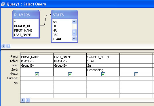
Database design
When building a relational database from scratch, it is important that you put good deal of thought into the process. A poorly designed database can cause a number of headaches for its users, including:
- loss of data integrity over time
- inability to support needed queries
- slow performance
Entire courses can be spent on database design concepts, but we don't have that kind of time, so let's just focus on some basic design rules that should serve you well. A well-designed table is one that:
- represents a single subject;
- has a primary key (a field or set of fields that uniquely identifies each record in the table);
- does not contain multi-part fields (e.g., "302 Walker Bldg, University Park, PA 16802");
- does not contain multi-valued fields (e.g., an Author field shouldn't hold values of the form "Jones, Martin, Williams");
- does not contain unnecessary duplicate fields (e.g., avoid using Author1, Author2, Author3);
- does not contain fields that rely on other fields (e.g., don't create a Wage field in a table that has PayRate and HrsWorked fields);
- contains a minimum of redundant data.
Let's work through an example design scenario to demonstrate how these rules might be applied to produce an efficient database. Those ice cream entrepreneurs, Jen and Barry, have opened their business and now need a database to track orders. When taking an order, they record the customer's name, the details of the order such as the flavors and quantities of ice cream needed, the date the order is needed, and the delivery address. Their database needs to help them answer two important questions:
- Which orders are due to be shipped within the next two days?
- Which flavors must be produced in greater quantities?
A first crack at storing the order information might look like this:
| Customer | Order | DeliveryDate | DeliveryAdd |
|---|---|---|---|
| Eric Cartman | 1 vanilla, 2 chocolate | 12/1/08 | 101 Main St |
| Bart Simpson | 10 chocolate, 10 vanilla, 5 strawberry | 12/3/08 | 202 School Ln |
| Stewie Griffin | 1 rocky road | 12/3/08 | 303 Chestnut St |
| Bart Simpson | 3 mint chocolate chip, 2 strawberry | 12/5/08 | 202 School Ln |
| Hank Hill | 2 coffee, 3 vanilla | 12/8/08 | 404 Canary Dr |
| Stewie Griffin | 5 rocky road | 12/10/08 | 303 Chestnut St |
The problem with this design becomes clear when you imagine trying to write a query that calculates the number of gallons of vanilla that have been ordered. The quantities are mixed with the names of the flavors and any one flavor could be listed anywhere within the order field (i.e., it won't be consistently listed first or second).
A design like the following would be slightly better:
| Customer | Flavor1 | Qty1 | Flavor2 | Qty2 | Flavor3 | Qty3 | DeliveryDate | DeliveryAdd |
|---|---|---|---|---|---|---|---|---|
| Eric Cartman | vanilla | 1 | chocolate | 2 | 12/1/08 | 101 Main St | ||
| Bart Simpson | chocolate | 10 | vanilla | 10 | strawberry | 5 | 12/3/08 | 202 School Ln |
| Stewie Griffin | rocky road | 1 | 12/3/08 | 303 Chestnut St | ||||
| Bart Simpson | mint chocolate chip | 3 | strawberry | 2 | 12/5/08 | 202 School Ln | ||
| Hank Hill | coffee | 2 | vanilla | 3 | 12/8/08 | 404 Canary Dr | ||
| Stewie Griffin | rocky road | 5 | 12/10/08 | 303 Chestnut St |
This is an improvement because it enables querying on flavors and summing quantities. However, to calculate the gallons of vanilla ordered, you would need to sum the values from three fields. Also, the design would break down if a customer ordered more than three flavors.
Slightly better still is this design:
| Customer | Flavor | Qty | DeliveryDate | DeliveryAdd |
|---|---|---|---|---|
| Eric Cartman | vanilla | 1 | 12/1/08 | 101 Main St |
| Eric Cartman | chocolate | 2 | 12/1/08 | 101 Main St |
| Bart Simpson | chocolate | 10 | 12/3/08 | 202 School Ln |
| Bart Simpson | vanilla | 10 | 12/3/08 | 202 School Ln |
| Bart Simpson | strawberry | 5 | 12/3/08 | 202 School Ln |
| Stewie Griffin | rocky road | 1 | 12/3/08 | 303 Chestnut St |
| Hank Hill | coffee | 2 | 12/8/08 | 404 Canary Dr |
| Hank Hill | vanilla | 3 | 12/8/08 | 404 Canary Dr |
| Stewie Griffin | rocky road | 5 | 12/10/08 | 303 Chestnut St |
This design makes calculating the gallons of vanilla ordered much easier. Unfortunately, it also produces a lot of redundant data and spreads a complete order across multiple rows.
Better than all of these approaches would be to separate the data into four entities (Customers, Flavors, Orders, and Order Items):
If one were to implement a design like this in MS-Access, the query needed to display orders that must be delivered in the next 2 days would look like this in the GUI: 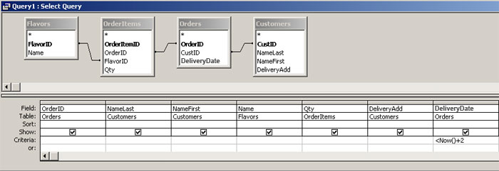
It would produce the following SQL: SELECT Orders.OrderID, Customers.NameLast, Customers.NameFirst, Flavors.Name As Flavor, If you aren't experienced with relational databases, then such a table join may seem intimidating. You probably won't need to do anything quite so complex in this course. The purpose of this example is two-fold:
Try This!To get some practice with building queries, work through this tutorial that references the same baseball statistics database utilized above.
|
Building a MySQL Database
In this part of the lesson, you'll learn methods for creating and populating tables in a MySQL database. Creating tables can be done using a web-based application called phpMyAdmin or a desktop application called MySQL Workbench. I will provide instructions for both applications.
After defining your tables, you'll download a special driver that will enable you to connect to the MySQL database using MS-Access. Using Access as a "front end," you'll have a user-friendly GUI for populating your MySQL tables and querying them.
Every step in this process could be completed using command-line SQL. (In fact, the GUI-based tools we'll be using simply generate and execute SQL code.) If you're an SQL expert, you're welcome to use SQL interfaces to complete these steps instead. My assumption is that most of you, like me, are not SQL experts and will find this methodology to be less frustrating.
MySQL Data Types
The data types used in MySQL for storing text strings are:
- CHAR: used for columns with values of an exact length
Ex: CHAR(2) for state abbreviations like "PA" and "NY"
- VARCHAR: used for columns with values of variable lengths up to 255
Ex: VARCHAR(25) for names - TEXT: used for free-form text such as comments of up to ~65000 characters
- MEDIUMTEXT: free-form text of up to ~1.6 million characters
- LONGTEXT: free-form text of up to ~4 trillion characters
The data types for storing integers are shown in the table below. As the table shows, columns of these types can be signed or unsigned. Unsigned columns can only hold positive values. Signed columns can hold both positive and negative values.
| Type | Signed Range | Unsigned Range |
|---|---|---|
| TINYINT | -128 to 128 | 0 to 255 |
| SMALLINT | -32768 to 32767 | 0 to 65535 |
| MEDIUMINT | -8.3M to 8.3M | 0 to 16M |
| INT | -2.1B to 2.1B | 0 to 4.2B |
| BIGINT | > ±2.1B | > 4.2B |
For numbers that have digits after the decimal point, there are two main data types:
- FLOAT: used for numbers with up to 7 significant digits
- DOUBLE: used for numbers with up to 16 significant digits
The data type limits above are approximate in many cases. To find more specific limits and to see other supported data types such as those dealing with dates and times, refer to the MySQL documentation [186].
Defining Tables
For this Jen and Barry's demonstration project, we're going to create three tables:
|
|
|
You can define these tables using either phpMyAdmin or the MySQL Administrator:
- Using phpMyAdmin
To connect to your database:- In a web browser, go to phpMyAdmin [187].
- Enter the Username and Password found in the file named dbinfo at the root of your personal web space (e.g., I can view my file at http://www.personal.psu.edu/jed124/dbinfo [188]). Your database username is the second item in the file; your password is the third.
- After you've successfully logged in, you need to select which database you want to work with. To do this, click on the Databases button at the top of the screen, then on the database that's named the same as your PSU access account ID.
To create a table:- When entering a database page, you’ll see a section of the page labeled Create new table on database <your access account ID>. In this case, enter candidate_cities in the Name box and 4 in the Number of fields box. Then click the Go button on the right side of the window.
- You should see 4 rows of textboxes, one for each field you said you wanted to create. Enter name in the first Field box.
- From the Type drop-down list, select VARCHAR.
- In the Length/Values box, enter 25.
- Repeat the previous 3 steps to add the population, x and y columns to the table (keeping in mind that numeric fields don’t require a “Length/Values” setting).
- After you've entered all of the field settings, click the Save button in the lower right of the window.
- Click on the Database link at the top of the page to create more tables.
- Repeat the steps above to add the other two tables (counties and county_geom) to your database.
- Using MySQL Workbench
To install MySQL Workbench:- Browse to MySQL Workbench [189].
- Near the bottom of the page, click the Download button next to Windows (x86, 32-bit) MSI Installer.
- Create a MySQL.com account if you like or click No thanks, just take me to the downloads!
- Click the HTTP link of the server nearest you to begin download.
- Run the downloaded .msi file and follow the on-screen directions.
To connect to your database:- Open MySQL Administrator (Start > MySQL > MySQL Workbench).
- Under the SQL Development heading, click the New Connection option.
- In the Setup New Connection dialog, enter a Connection Name of your choosing (such as PSU PHPDB).
- Enter the Hostname: instructdb3.ait.psu.edu.
- Enter the Username found in the file named dbinfo at the root of your personal web space (e.g., I can view my file at http://www.personal.psu.edu/jed124/dbinfo [188]) and click OK. Your database username is the second item in the file; your password is the third. The Setup New Connection dialog will disappear and you should see your connection listed in the box under the SQL Development heading.
- Click the Open Connection to Start Querying option just above the box. A Connect to Database dialog should appear.
- Select the connection you just created from the Stored Connection list. The Hostname and Username boxes should be populated with your connection parameters automatically.
- Click OK and then enter the password found in your dbinfo file when prompted. You should see a schema (i.e., a database) with your user ID and beneath it a list of Tables, Views and Routines (each list being empty at this point).
To create a table:- Click the Create a New Table button just above the large schema heading near the middle of the window. (It is the 3rd of 5 buttons.) A new_table dialog will appear with a number of tabs running along the bottom.
- Under the Table tab, give the table the name candidate_cities.
- Switch to the Columns tab where you should see a cursor flashing in a text box beneath the Column Name heading.
- Enter name in the text box (this column will hold the names of the cities), then hit Tab or Enter.
- Set the column's Datatype to VARCHAR(25).
- Double-click the empty space under the column you just defined to begin defining a new column.
- Repeat steps 3-5 to add the other three candidate_cities columns.
- Repeat the steps above to add the other two tables (counties and county_geom) to your database.
- Right-click on the idnew_table column that was defined by default and select Delete Selected Columns.
- Click Apply, then Apply SQL and Finish to create the table.
- When done creating tables, click Close to dismiss the new_table dialog.
Although we didn't need them in this scenario, you may have noticed the checkboxes to the right of the Datatype heading. I won't go through all of them, but the ones that I've used most often are PK (to declare a column as a primary key), NN (to disallow Null values in a column), AI (to automatically increment the value in that column by 1 when a new record is added), and Default (to specify the default value assigned to the column when a new record is added).
Later in the lesson, we'll populate these tables. As you might have guessed, name is the key field in the two county tables that will allow us to join the attribute information with the geometries. If you were to build a real mashup in this sort of scenario, I would recommend using a column of shorter length (preferably a numeric column, like the U.S. Census Bureau's FIPS) as the key field. When we populate the county_geom table with the vertices of the features in the counties shapefile, it will have over 5600 records (107 vertices for Thompson County, 44 for Viceroy County, etc.) Each vertex record will contain the name of its parent county. This is a needless waste of space, and probably more importantly, table joins and sorts based on long character strings such as these perform more slowly than those based on numeric IDs. The shapefile didn't include a shorter ID and I don't think it's worth the effort to add one, so just keep in mind that we're not following a best practice here.
Installing the MySQL ODBC driver
This part of the process involves downloading and installing a driver that will enable you to view MySQL data within a Microsoft product, such as Access.
- Download the appropriate driver at: http://dev.mysql.com/downloads/connector/odbc/ [190]. Getting the right driver/combination of drivers has been tricky for some folks in the past. If you're on a 64-bit machine, I suggest starting with the 64-bit driver. If the connection steps below don't work, try installing the 32-bit driver too (leaving the 64-bit driver installed). If you're on a 32-bit machine, I think the 32-bit driver by itself should work.
- Under Windows downloads, click Pick a mirror.
- Create a MySQL.com account if you like or click No thanks, just take me to the downloads!
- Click the HTTP link of the server nearest you to begin download.
- Run the downloaded .msi file and follow the on-screen directions.
Setting up an ODBC connection
In this part of the tutorial, you'll specify parameters that can be used by Access to connect to your MySQL database.
- Open the ODBC Data Source Administrator by going to:
- Start > Control Panel > Administrative Tools > Data Sources (XP).
- Start > Control Panel > System and Maintenance > Administrative Tools > Data Sources (Vista).
- Start > Control Panel > System and Security > Administrative Tools > ODBC Data Sources (Windows 7/8).
- Under the User DSN tab, click Add.
- In the Create New Data Source dialog, select the MySQL ODBC 5.x DRIVER (should be near the bottom of the list) and click Finish.
- In the resulting dialog, make the following settings:
- Data Source Name: mysql_<your PSU access account ID> (or any name of your choice)
- TCP/IP Server: instructdb3.ait.psu.edu
- User: found in your dbinfo file
- Password: found in your dbinfo file
- Select your database from the Database drop-down list. If you receive an error message, double-check your settings.
- Click OK to save the connection settings. You should see your data source listed under the User DSN tab and can dismiss the ODBC Data Source Administrator window and close the Administrative Tools window.
Linking to your MySQL tables in MS-Access
- In Access 2003:
- Open Microsoft Access and select File > New.
- In the New File dialog box, select Blank Database.
- Specify a name (like mysql_jenbarry.mdb) and location for your database and click Create.
- With the new Access database opened, select Tables from the Objects list.
- Click New, then Link Table.
- In the Files of type field, select ODBC Databases.
- Select your ODBC connection under the File Data Source tab and click OK.
- Enter your MySQL User ID and Password and click OK.
- Select the three tables created in MySQL above and click OK.
You'll be prompted to select a primary key for each table by picking a column (or combination of columns) that uniquely identifies each record. Note that you must select a primary key if you plan to add or modify data in the table. If you will not be altering the table's records, you can just click OK. - Select NAME as the unique identifier for the candidate_cities and counties tables, and VID for the county_geom table.
- In Access 2007:
- Open Microsoft Access, and from the Getting Started window select Blank Database.
- In the Blank Database pane, specify a name (like mysql_jenbarry.accdb) and location for your database and click Create.
- The new database will open with a new blank table called Table1. Close this table.
- Click the External Data tab, then the More drop-down list in the grouping of buttons labeled Import.
- From the drop-down list, select ODBC Database.
- In the Get External Data dialog box, select Link to the data source... and click OK. This option will enable you to modify the data in the MySQL tables utilizing Access, whereas the Import the source data... option would create an unlinked snapshot of the MySQL data.
- Select your ODBC connection under the File Data Source tab and click OK.
- Select the three tables created above and click OK.
You'll be prompted to select a primary key for each table by picking a column (or combination of columns) that uniquely identifies each record. Note that you must select a primary key if you plan to add or modify data in the table. If you will not be altering the table's records, you can just click OK. - Select NAME as the unique identifier for the candidate_cities and counties tables, and VID for the county_geom table.
- In Access 2010:
- Open Microsoft Access, and from the Getting Started window select Blank Database.
- In the Blank Database pane, specify a name (like mysql_jenbarry.accdb) and location for your database and click Create.
- The new database will open with a new blank table called Table1. Close this table.
- Click the External Data tab, then ODBC Database.
- In the Get External Data dialog box, select Link to the data source... and click OK. This option will enable you to modify the data in the MySQL tables utilizing Access, whereas the Import the source data... option would create an unlinked snapshot of the MySQL data.
- Select your ODBC connection under the File Data Source tab and click OK.
- Select the three tables created above and click OK.
You'll be prompted to select a primary key for each table by picking a column (or combination of columns) that uniquely identifies each record. Note that you must select a primary key if you plan to add or modify data in the table. If you will not be altering the table's records, you can just click OK. - Select NAME as the unique identifier for the candidate_cities and counties tables, and VID for the county_geom table.
Populating a table through manual entry
The Jen and Barry's candidate_cities shapefile (the same dataset used in Lesson 3) contains only four records and just a few attributes, so its data can be entered manually.
- Load the shapefile into ArcMap and open its attribute table.
- Add two new Double fields to the attribute table named X and Y.
- Right-click on the X field header and select Calculate Geometry.
- Choose X Coordinate of Point from the Property list and confirm that the values will be in the GCS/NAD27 coordinate system and in Decimal Degree units. Click OK.
- Repeat this step to populate the Y field.
- Leaving ArcMap and the attribute table open, return to your Access database and open the candidate_cities table.
- Manually enter the values for the four candidate cities. You may notice a slight delay after entering a value and tabbing into the next cell. This is because the values must be transferred across the Internet to your MySQL database hosted at PSU, instead of being stored on a local disk.
Adding the X and Y coordinate values to the attribute table as outlined above is my recommended strategy when you are looking to transfer the coordinates of point features to a database. In the next section, we'll see how to insert records into a MySQL table in bulk, rather than manually. Later, we'll see how to transfer the coordinates of line or polygon features to a database.
Populating a table using an SQL query
The query writing tutorial you completed earlier in the lesson had you dealing exclusively with SELECT queries. We're now going to add the county feature attributes to the database by importing a copy of the shapefile's DBF table and writing what Access calls an Append query to add values from selected columns in the local counties table to the MySQL counties table.
- Access 2003:
- In Access, click New in the database window, then select Import Table and click OK.
- In the Files of type drop-down list, select any of the dBASE (dbf) options.
- Browse to the location of the Jen and Barry's counties shapefile, select the counties.dbf table and click Import. After the table has been successfully imported, click Close.
- Double-click on the counties table to open it and confirm that the values imported correctly. Note that the icon beside the counties table in the database window indicates a table whose values are stored locally as part of the .mdb file, whereas the icon beside the tables added earlier indicates a linked table whose values are stored in some other database.
- Now, select Queries from the Objects list.
- Double-click on Create query in Design view.
- In the Show Tables dialog, double-click on counties to add that table to the query, then click Close.
- Just to the left of the Run button (exclamation point icon) is a pull-down menu. Select Append Query from this menu. Upon making this selection, you're asked to specify which table you want to append values to.
- Select the linked MySQL counties table from the Table Name drop down list and click OK. Note that an Append To row is added to the design grid between the Sort and Criteria rows.
- Double-click on the NAME field from the local counties table to add that field to the design grid. Note that NAME is also automatically entered as the Append To value. What's happened here is that Access scanned through the MySQL counties table for a field by the same name. It found one, so it made the assumption that you wanted to append the values to that field.
- Double-click on the AGE_18_64 field from the local counties table to add that field to the design grid. Note that in this case, nothing appears in the Append To area of the design grid because there is no field by that name in the MySQL table.
- In the design grid, click in the Append To cell under the AGE_18_64 column and then select WORKFORCE from the drop-down list.
- Repeat the step above to specify that you want to append values from the NO_FARMS87 and POP_SQMILE fields in the local counties table to the FARMS and POP_DENSITY fields in the MySQL counties table.
- Click the Run button to execute the query. You should receive a confirmation message asking if you really want to append 43 records. Click Yes.
- Open the MySQL counties table and confirm that the values were appended correctly. Once satisfied that your MySQL counties table has been populated properly, the local counties table is no longer needed.
- Go back to Tables in the database window, right-click on the local counties table and select Delete.
- Access 2007/2010:
- In Access, click the External Data tab, then click on the More drop-down menu in the grouping of controls labeled Import. Select dBASE File from that menu.
- In the Get External Data dialog, click the Browse button to locate the counties.dbf file, then click OK to import the data. After the table has been successfully imported, click Close.
- Double-click on the counties table in the Navigation Pane to open it and confirm that the values imported correctly. Note that the icon beside the counties table in the Navigation Pane indicates a table whose values are stored locally as part of the .mdb file, whereas the icon beside the tables added earlier indicates a linked table whose values are stored in some other database.
- Now, create a new query by clicking the Create tab and the Query Design button.
- In the Show Tables dialog, double-click on counties to add that table to the query, then click Close.
- In the group of controls labeled Query Type, click the Append button. Upon making this selection, you're asked to specify which table you want to append values to.
- Select the linked MySQL counties table from the Table Name drop down list and click OK. Note that an Append To row is added to the design grid between the Sort and Criteria rows.
- Double-click on the NAME field from the local counties table to add that field to the design grid. Note that name is also automatically entered as the Append To value. What's happened here is that Access scanned through the MySQL counties table for a field by the same name. It found one, so it made the assumption that you wanted to append the values to that field.
- Double-click on the AGE_18_64 field from the local counties table to add that field to the design grid. Note that in this case, nothing appears in the Append To area of the design grid because there is no field by that name in the MySQL table.
- In the design grid, click in the Append To cell under the AGE_18_64 column and then select WORKFORCE from the drop-down list.
- Repeat the step above to specify that you want to append values from the NO_FARMS87 and POP_SQMILE fields in the local counties table to the FARMS and POP_DENSITY fields in the MySQL counties table.
- Click the Run button to execute the query. You should receive a confirmation message asking if you really want to append 43 records. Click Yes.
- Open the MySQL counties table and confirm that the values were appended correctly. Once satisfied that your MySQL counties table has been populated properly, the local counties table is no longer needed.
- Right-click on the local copy of the counties table in the Navigation Pane and select Delete.
Note
Look at the SQL code generated by the GUI and note that what Access refers to as an Append query is actually an INSERT query in standard SQL syntax. Though we didn't do it in this tutorial, other attributes of polygon features that you might want to consider storing in a mashup database are the centroid coordinates of the polygons. These values can be added to the attribute table using the same ArcMap Calculate Geometry command utilized above. Those polygon centroid coordinates could then be used to label the polygons with custom markers in lieu of using a third-party labeling extension.
Transferring line/polygon coordinates to a database
Unlike point features that have a 1:1 relationship between their geometries and their attribute table records, line and polygon features have multiple x/y coordinate pairs (vertices) associated with each attribute table record. Thus, the Calculate Geometry method outlined above cannot be used to transfer line/polygon geometries to a database.
In an earlier lesson, you used a custom tool written in Python to export the coordinates of features to an XML file. We're now going to use the other tool in that toolbox to export those coordinates to a comma-separated-values (.csv) text file. This csv file can then be imported into Access and its values appended to the appropriate MySQL table, just as we did in the previous section with the county attributes.
- In ArcToolbox, open the Mashup Tools toolbox and run the Export Shapefile to CSV tool.
- For the Layer parameter, browse to the Jen and Barry's counties shapefile.
- For the ID Field parameter, select the NAME field.
Note
Unlike the XML tool, the CSV tool only allows for the selection of one field instead of many. This is based on the assumption that other attributes can be added to the database by importing the attribute table itself as described in the previous section.
- Click OK to perform the export, then click Close to dismiss the results dialog.
- Import the CSV file into your Access database as outlined above. (Keep in mind that you're importing a Text File rather than a dBASE File.)
- Again following the steps laid out in the previous section, append the coordinate records from the local table to the linked MySQL county_geom table.
Note
The coordinate fields in the CSV file will be labeled Lat and Lon. Be sure you match these fields up correctly with the fields in the MySQL table: Lat = Y, Lon = X. The file also includes a Part value. This is required for multi-part polygon features (such as the state of Hawaii). None of the counties in the Jen and Barry's scenario have multiple parts, so this value will be 1 for every record.
With that, you've completed the first step in constructing a database-driven mashup. The next step is to write a server-side script to extract the necessary data from the database and feed it to a JavaScript program much like what you've already written. The PHP language is often used for reading data from a database, so that is what we'll be using. The next part of the lesson talks about PHP generically and gives you some practice writing basic PHP scripts. Later in the lesson, we'll come back to this database and see how PHP can be used to retrieve data from it.
PHP
PHP is a recursive acronym – an abbreviation referring to itself – that stands for PHP Hypertext Preprocessor. It is a free and open-source web scripting language that, like JavaScript, is intermixed with HTML in a web page to generate content on the fly. Unlike JavaScript, PHP code must be executed by a web server as opposed to by the machine viewing the page. This is why PHP is often referred to as a server-side language, while JavaScript is referred to as a client-side language. The PHP website [191] and the PHP Tutorial from the w3schools website [192] are good resources for tutorials and language documentation for PHP.
A basic PHP file looks something like this:
| <html> <head> <title>PHP example</title> </head> <body> <?php echo “Hello world”; ?> </body> </html> |
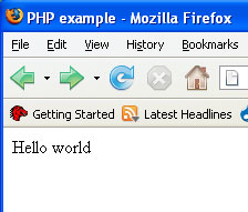 |
Important items to note in looking at this example are:
- PHP code is embedded within the HTML code.
- PHP code is enclosed within the <?php and ?> tags.
- The echo keyword is used to output a string. (Print may also be used in place of echo.)
- All PHP statements must end with a semicolon. (Unlike JavaScript, in which the ending semicolon is optional.)
- The document must be saved with a .php extension. This ensures that the server interprets and executes the PHP code in the file before sending the page to the client.
Note that either of the following alternatives can be used to produce the same result:
| <html> <head> <title>PHP example</title> </head> <body> <?php echo “<strong>Hello world</strong>”; ?> </body> </html> |
<html> |
Comments in PHP
As with other programming languages, PHP programmers can add comments to their code to make it easier to follow or to "comment out" code that isn't working. The short example below shows how to add a single-line comment and a comment block.
  <html>
    <body>
      <?php
        // This is a comment

        /*
        This is
        a comment
        block
        */
      ?>
    </body>
  </html>
Variables in PHP
As in JavaScript, variables in PHP are untyped - meaning a developer need not specify a data type when beginning to use a variable. Unlike JavaScript, variables cannot be declared using a keyword like var. They are simply created using a name beginning with the $ character and referenced as in the example below:
<html>
  <head>
    <title>PHP example</title>
  </head>
  <body>
    <?php
      $msg = "Hello World";
      echo $msg;
    ?>
  </body>
</html>
The first character after the $ must be either a letter or an underscore (not a number).
PHP string concatenation
Whereas JavaScript uses the + operator to concatenate strings, PHP uses the . (period). See the example below:
<html>
  <head>
    <title>PHP example</title>
  </head>
  <body>
    <strong>
    <?php
      $last = ‘Mouse’;
      $first = ‘Mickey’;
      echo $first . $last;
    ?>
    </strong>
  </body>
</html>
PHP operators
All of the following PHP operators work the same as they do in JavaScript (notes added in parentheses for those that may not be obvious to you):
| Arithmetic |
+, -, *, /, ++ (increment by 1), -- (decrement by 1) |
| Comparison | == (equals), != (not equals), >, <, >=, <= |
| Logical | && (and), || (or), ! (not) |
One area of difference in operators between the two languages is the concatenating assignment operator, which is often used to append additional text onto an existing string variable. For example, given a JS variable called x containing the string "Hello", additional text can be appended to x using the statement:
x += " World";
This syntax is often used in place of:
x = x + " World";
As you might guess, the PHP equivalent of the "+=" operator is ".=":
$x .= " World";
Conditional statements in PHP
The basic syntax of an if construct is the same as in JavaScript. The if condition must be placed in parentheses and all statements to be executed under the condition must be enclosed within braces. The only difference is that the "else if" construct is one word instead of two words:
if ($temp < 32) {
   echo “It’s freezing!”;
}
elseif ($temp > 90) {
   echo “It’s too hot!”;
}
else {
   echo “It’s comfortable.”;
}
PHP arrays
An array can be created in PHP using the following syntax:
$states = array("PA", "NY", "NJ", "DE");
Obtaining an individual array element is done by specifying the position of the element in brackets:
echo $states[0];
Loops in PHP
PHP offers two main types of loops (while and for) whose syntax and behavior is the same as in JavaScript. while is used to execute a block of code as long as some condition is met:
$i=1;
while($i<=5) {
  echo "The number is " . $i . "<br />";
  $i++;
}
for is used to execute a block of code a certain number of times:
for ($i=1; $i<=5; $i++) {
  echo “The number is “ .$i . “<br />”;
}
PHP's date() function
Of the many functions built into PHP, one of the more useful is date(), which is used to display both dates and times in various formats. The key to using the date() function is supplying a string argument that specifies the desired format. The following examples demonstrate its use:
| Code | Example Result |
| echo "Today is " .date("l"); | Today is Monday |
| echo "The date is " .date("n/j/Y"); | The date is 11/3/2008 |
| echo "The current time is " .date("g:i:s a"); | The current time is 4:04:25 pm |
A complete list of formatting characters can be found at w3schools [193].
The date() function can also be used to format dates other than the current date. This is done by supplying a timestamp for the function's optional second parameter. A timestamp is the number of seconds since midnight, January 1, 1970. Assuming you don't know that value off the top of your head, you can calculate it using the mktime() function. The syntax of this function is: mktime(hour, minute, second, month, day, year). The following example demonstrates using the date() and mktime() functions together:
echo “July 4th, 2020 is a “ . date(“l”, mktime(0,0,0,7,4,2020));
String functions in PHP
Like other programming languages, PHP provides a number of functions that are used to manipulate strings. Some of the more useful of these include:
- strlen() — returns the length of a string
- strpos() — returns the position of one string inside another
- strtolower() — converts a string to lower-case
- strtoupper() — converts a string to upper-case
- substr() — returns part of a string
Again, a more complete listing of PHP string functions can be found at w3schools [194].
PHP practice exercises
To help you gain a bit of comfort with PHP before we dive into its use in retrieving data from a database, please complete the following practice exercises. For each of the exercises, be sure to save your code with a .php extension and upload it to the special php folder in your personal web space to test it.
Note
While the www.personal.psu.edu [195] server is configured to handle PHP scripts, it's not able to connect to the MySQL databases that have been set up for us. For that purpose, we'll use the phpdb.aset.psu.edu server instead. Although these practice exercises don't involve a database, to avoid confusion I'm going to recommend you use the phpdb server to execute all of your PHP scripts. This server is configured such that you can omit your access account ID from the URL. For example, I uploaded a script called date_function.php to my phpjed124 folder. I can execute that script and view its output using the URL https://phpdb.aset.psu.edu/phpjed124/date_function.php [196]. You can follow the same pattern to execute your scripts.
- Create three variables (x, y, and z). Assign a value of 9 to x, a value of 7 to y and then make z equal to the sum of those two variables. Display the contents of the z variable on the screen using an echo statement.
Solution to Practice Exercise 1 [197] - Use the date() function to display your birthday in the following format:
Friday, December 5, 2008
Solution to Practice Exercise 2 [198]
In this part of the lesson, you read about PHP and got some practice with it. In the next part, you'll read a brief bit on the topic of setting up HTML forms to accept input from the user and accessing that input within your PHP scripts.
Reading from a MySQL Database with PHP
PHP's database support
PHP is a popular open-source language for building web pages that draw dynamic content from a database. It has functions for extracting data from all of the major RDBMS packages. This part of the lesson focuses on using PHP with MySQL. If you're considering retrieving data from a package other than MySQL, you should visit PHP's Database Extensions page [199].
The University server we're using in this course is actually equipped with the MySQL Improved Extension (MySQLi) [200] rather than the older MySQL Extension [201]. The old extension enables interaction with a database through a set of functions whose names begin with mysql_. Generally speaking, the improved extension has all of the same functions, just with names beginning instead with mysqli_. One of the improvements the MySQLi extension offers developers is the ability to write code in an object-oriented or a procedural style. My experience has been with the original MySQL Extension, which is strictly procedural, and I have not yet had a chance to experiment with the object-oriented style. Therefore, my examples are written in the procedural style. You are welcome to write object-oriented code if you'd prefer.
In looking at the reference documentation on the php.net site, it appears that it is geared toward those using the object-oriented style. Because this could make it harder for you to follow my examples, I'm going to refer you instead to another site that appears to be hosting an older version of the reference documentation that I've found easier to follow. For example, the first function we'll use is called mysqli_connect(). You can find a description of this function at this site: PHP Manual:mysqli-connect [202]. You can also jump to descriptions of any of the other mysqli_ functions used in the lesson by clicking on their links. Unfortunately, finding this same function in the php.net version of the documentation is much more difficult because it's listed under the heading of mysqli::__construct (the object-oriented version of the function). This is just one example of why I'm directing you away from the current documentation at php.net.
Connecting to MySQL with PHP
Using the MySQLi Extension, connections are made to MySQL databases using the mysqli_connect() function (reference documentation cited above). This function accepts 6 optional arguments, the first 4 of which we'll need in this class: the name of the server hosting the database, the user's name, the user's password and the name of the database. It returns a link to the database that is needed by other mysqli functions (e.g., the one needed to execute SQL queries). I would make a connection to my database and store the returned link in a variable like this:
<?php
$link = mysqli_connect("instructdb3.ait.psu.edu","inst_4","password","jed124");
?>
When connecting to your database, you should replace my database name (access account ID) with yours and replace my user name and password with the values supplied to you in the dbinfo file that was put in your personal web space.
Writing SQL to retrieve the desired data
This stage of the mashup building process is another of the reasons I recommend using Access as a front-end to your MySQL database. Its query building GUI can be an effective tool for generating the SQL needed by a mashup, particularly if the query requires joins or group by operations. For example, if my PHP script needed a career home run list from a MySQL version of the baseball stats database, I'd use Access to build the query much like you did during the SQL tutorial. I'd then switch to SQL View and copy and paste the SQL code into my PHP script, storing the SQL string in a variable for use later.
There's just one problem with this methodology: the version of SQL employed by Access is of a slightly different dialect than that of MySQL. Some of these differences can be seen by comparing the same query in the two different dialects next to one another:
Access:
SELECT [players]![first_name] & ' ' & [players]![last_name] AS player, Sum(stats.hr) AS career_hr
FROM players INNER JOIN stats ON players.player_id = stats.player_id
GROUP BY [players]![first_name] & ' ' & [players]![last_name]
ORDER BY Sum(stats.hr) DESC;
MySQL:
SELECT CONCAT(players.first_name, ' ', players.last_name) AS player, Sum(stats.hr) AS career_hr
FROM players INNER JOIN stats ON players.player_id = stats.player_id
GROUP BY CONCAT(players.first_name, ' ', players.last_name)
ORDER BY Sum(stats.hr) DESC;
The difference that is likely to make the most impact on your query writing is the way that Access places table/field names inside brackets and the way that it signals a parent-child relationship between a table and field using an exclamation point. In the standard SQL used by MySQL, there are no brackets around table/field names and a parent table is connected to its child field using a period.
The other difference that can be seen in this example is that concatenation is done in MySQL using the CONCAT() function, whereas strings are concatenated in Access using an ampersand (&) or a plus sign (+).
More of the differences between Access SQL and MySQL SQL can be found at SQLzoo.net [203]. Despite the differences, I still find modifying the code generated by the Access query GUI easier than producing the code wholly from scratch, but your mileage may vary.
Plugging the MySQL-friendly version of the SQL into the PHP script looks like this:
<?php
$link = mysqli_connect("instructdb3.ait.psu.edu","inst_4","password","jed124");

$sql = "SELECT CONCAT(players.first_name, ' ', players.last_name) AS player,
   Sum(stats.hr) AS career_hr
   FROM players INNER JOIN stats ON players.player_id = stats.player_id
   GROUP BY CONCAT(players.first_name, ' ', players.last_name)
   ORDER BY Sum(stats.hr) DESC;";
?>
Executing the SQL
The next step is to execute the query held in the $sql variable using the mysqli_query() function. mysqli_query() requires a database link for its first argument and a query string for its second argument. When executing a SELECT query as we're doing here, mysqli_query() returns a result object, which like the database link, should be stored so that it can be used later by other mysqli functions:
$result = mysqli_query($link, $sql);
Note
If there is an error in your query syntax, mysqli_query() will return a value of FALSE instead of a result object. Also keep in mind that your query may have perfectly valid syntax, but yield no records because of either flawed logic in the query's design or a simple lack of data meeting the criteria at that time. An example of flawed logic would be a query that attempts to select records having an hr value less than 0 (which is impossible). An example of the second situation would be a query that attempts to select records where the last_name is 'Rodriguez'. There are no records presently in the database meeting that criterion (though if I were to re-populate the database with the current top 10 home run hitters, there would be). In both cases, the query will return a result object because of its valid syntax, but it will contain 0 rows. (See the usage of the mysqli_num_rows() function below.)
Obtaining the query results
The mysqli_fetch_array() function can be used to obtain one row of data from your query result. The values in that row are returned as an array, which is typically stored in a variable. An individual value can then be obtained from the array variable by supplying the name of a column in brackets. For example:
$row = mysqli_fetch_array($result);
$player = $row['player'];
// OR
// $player = $row[0]; // assuming "PLAYER" is 1st field
There are two main ways to process all of the records returned by a query. The first involves determining how many records were returned using the mysqli_num_rows() function, then setting up a for loop to carry out the necessary processing that many times. The other method involves taking advantage of the fact that mysqli_fetch_array() returns 0 if the last row has already been fetched. With this method, a while loop can be used to continue processing until mysqli_fetch_array() returns 0. Both methods are demonstrated below, with the while loop commented out:
$num_results = mysqli_num_rows($result);
for ($i=0;$i<$num_results;$i++) {
   $row = mysqli_fetch_array($result);
   $player = $row['player'];
   $hr = $row['career_hr'];
   echo $player .', '. $hr .'<br />';
}

// OR
//while ($row = mysqli_fetch_array($result)) {
// $player = $row['player'];
// $hr = $row['career_hr'];
// echo $player .', '. $hr .'<br />';
//}
The second method is a bit more slick, though if you find it harder to follow, you're welcome to utilize the first method, which is a bit more straightforward.
The complete career home run script [204]is below (http://phpdb.aset.psu.edu/phpjed124/career_hr.php [204]) Note that the script includes a check of the $result variable to make sure the query returned a result. Note also the last line of the script which closes the connection to the database.
$link = mysqli_connect("instructdb3.ait.psu.edu","inst_4","password","jed124");

$sql = "SELECT CONCAT(players.first_name, ' ', players.last_name) AS player,
   Sum(stats.hr) AS career_hr
   FROM players INNER JOIN stats ON players.player_id = stats.player_id
   GROUP BY CONCAT(players.first_name, ' ', players.last_name)
   ORDER BY Sum(stats.hr) DESC;";
$result = mysqli_query($link,$sql);
if ($result != 0) {
   $num_results = mysqli_num_rows($result);
   for ($i=0;$i<$num_results;$i++) {
      $row = mysqli_fetch_array($result);
      $player = $row['player'];
      $hr = $row['career_hr'];
      echo $player .', '. $hr .'<br />';
   }
} else {
   echo 'Problem with query!';
}

mysqli_close($link);
Note
When running a PHP script that reads from your MySQL database, be sure to use the phpdb.aset.psu.edu server as shown in the URL above. It is specially configured to read data from our MySQL databases, whereas php.scripts.psu.edu is not.
Incorporating data from a database into a mashup
To convert a mashup based on a local XML file (like what was demonstrated earlier in the lesson) to one based on data coming from a database, there are really only two main steps:
- Write a PHP script using the methodology described above and output the data values in XML format.
- Change the ajax() statement so that it reads the XML produced by the PHP script instead of from the XML file.
Here is the source code for a PHP script that reads the candidate cities data from my MySQL database and outputs the values as XML [205] (http://phpdb.aset.psu.edu/phpjed124/get_cities.php [205]):
<?php
$link = mysqli_connect("instructdb3.ait.psu.edu","inst_4","password","jed124");

$sql = "SELECT name, population, x, y FROM candidate_cities ORDER BY name;";

$result = mysqli_query($link,$sql);
if ($result != 0) {
   header("Content-type: text/xml");
   echo '<shapes>';

   $num_results = mysqli_num_rows($result);
   for ($i=0;$i<$num_results;$i++) {
      $row = mysqli_fetch_array($result);
      $name = $row['name'];
      $pop = $row['population'];
      $x = $row['x'];
      $y = $row['y'];

      echo '<pt name="' .$name. '" population="' .$pop. '" x="' .$x. '" y="' .$y. '" />';
   }

   echo '</shapes>';
} else {
   echo 'Problem with query!';
}

mysqli_close($link);

?>
The statements to pay particular attention to are in bold. First, a header statement is added so that browsers receiving the output from this script will know that it is in XML format. Next, the start tag for the root element of the XML data is echoed to signal the beginning of the XML packet. Then inside the loop the current city's attributes are echoed in XML form.
This line can be tricky as it involves the use of both single and double quotes and a lot of concatenation. The literal text being echoed is in single quotes, but part of that literal text is a number of double quotes (because the values that are being retrieved from the variables represent element attribute values in the XML output and such values must be enclosed in quotes) . Perhaps the best way to produce a statement like this is to forget about quoting the attribute values at first, then add those quotes in later. Here is the statement without the attribute value quotes (i.e., no double quotes):
echo '<pt name=' .$name. ' population=' .$pop. ' x=' .$x. ' y=' .$y. ' />';
And here is the statement with caret symbols in place of where the double quotes ought to be (since it may be hard for you to differentiate between single and double quotes when they're right next to each other):
echo '<pt name=^' .$name. '^ population=^' .$pop. '^ x=^' .$x. '^ y=^' .$y. '^ />';
With the PHP script written, the next step is to modify the JavaScript you used earlier in the lesson so that it reads the output from the PHP script instead of an actual XML file:
$.ajax({ url: "get_cities.php", dataType: "xml", success: function(xmlDoc){
Because of the restriction that JavaScript can only read files in the same directory, you'll need to store your html page in the same folder as the PHP script. This means you may also need to copy your custom marker icons to the special PHP folder as well, or specify absolute paths to them in your code.
Polygon data example
Earlier in this lesson, I guided you through loading polygon attributes and geometries into MySQL. Now let's see how to retrieve polygons from MySQL and display them on a map.
The example page we're going to examine displays two maps of political party registration in Pennsylvania's 67 counties [206]: one depicting numbers from December 2007 and the other from April 2008, just before the state's presidential primaries.
First, have a look at the three tables involved in this mashup:
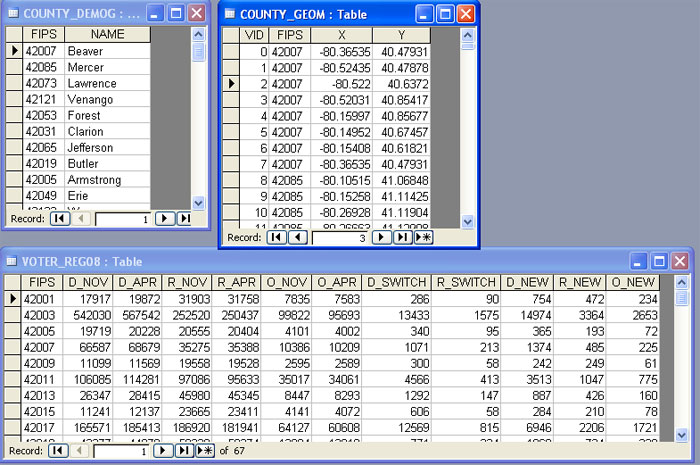
Note that each table contains a FIPS field, which is used to conduct joins between the tables. Now, let's look at the PHP script that's used to retrieve the required data [207](http://phpdb.aset.psu.edu/phpjed124/voter_reg.php [207]):
<?php
$link = mysqli_connect("instructdb3.ait.psu.edu","inst_4","password","jed124");

$sql = "SELECT COUNTY_DEMOG.FIPS, COUNTY_DEMOG.NAME, VOTER_REG08.D_NOV,
    VOTER_REG08.D_APR, VOTER_REG08.R_NOV,
    VOTER_REG08.R_APR, VOTER_REG08.O_NOV, VOTER_REG08.O_APR,
    VOTER_REG08.D_SWITCH, VOTER_REG08.R_SWITCH,
    VOTER_REG08.D_NEW, VOTER_REG08.R_NEW, VOTER_REG08.O_NEW
    FROM COUNTY_DEMOG
    INNER JOIN VOTER_REG08 ON COUNTY_DEMOG.FIPS = VOTER_REG08.FIPS;";

$result = mysqli_query($link,$sql);
if ($result != 0) {
    header("Content-type: text/xml");
    echo '<shapes>';

    $num_results = mysqli_num_rows($result);
    for ($i=0;$i<$num_results;$i++) {
        $row = mysqli_fetch_array($result);
        $fips = $row['FIPS'];
        $name = $row['NAME'];
        $d_nov = $row['D_NOV'];    $d_apr = $row['D_APR'];
        $r_nov = $row['R_NOV'];    $r_apr = $row['R_APR'];
        $o_nov = $row['O_NOV'];    $o_apr = $row['O_APR'];

        echo '<poly name="' .$name. '" d_nov="' .$d_nov. '" d_apr="' .$d_apr. '"
          r_nov="' .$r_nov. '" r_apr="' .$r_apr. '"
          o_nov="' .$o_nov. '" o_apr="' .$o_apr. '">';

        $sql = "SELECT X, Y FROM COUNTY_GEOM WHERE FIPS='" .$fips. "' ORDER BY VID;";

        $coords = mysqli_query($link, $sql);
        if ($coords != 0) {
            $num_coords = mysqli_num_rows($coords);
              for ($j=0;$j<$num_coords;$j++) {
              $rec = mysqli_fetch_array($coords);
              $x = $rec['X'];
              $y = $rec['Y'];
              echo '<v x="' .$x. '" y="' .$y. '" />';
            }
        }

        echo '</poly>';
    }

    echo '</shapes>';
}
The basic idea behind this program is to query the voter_reg_08 table to get a list of all the counties along with their voter registration information. A for loop is used to step through this list one county at a time. Within the loop, the county's name and registration figures are echoed as an XML element called poly.
Also within that loop, another bit of SQL is used to query the county_geom table for the coordinates of the vertices that form the geometry of the county being processed by the loop. A second loop is then embedded within the first to cycle through the records in the coordinate list. These coordinates are then echoed as an XML element called v (short for vertex) which is a child element of the parent poly element.
After the internal loop is complete, the poly element is closed with its end tag. Likewise, after the external loop is complete, the root element (shapes) is closed with its end tag.
As for the JavaScript code used for the page, I recommend that you view its source to follow along with this discussion. Just as the PHP script used two loops to produce the XML output, the function embedded in the ajax() statement uses two each() to read the XML. The first loop works through all of the elements in the XML packet with the tag name poly. Within the loop, the raw voter counts are obtained for the current county and converted to percentages. From those percentages, the margin separating the two major parties is computed and passed to a function called get_color(), which returns a hexadecimal color value that varies depending on the margin (dark blue for heavily Democratic counties, dark red for heavily Republican counties, etc.).
Note
I used ColorBrewer [208] to obtain the color values.
After a bit of code concerned with constructing the tables below the maps, the coordinates for the current county are obtained by getting all of the child elements of the parent poly element (referenced by the rec variable) with the tag name v. Recall that a Polygon is constructed from an array of LatLng objects, so a new empty array variable called pts is created. This array variable is then populated by a second loop that steps through all of the v elements. For each vertex, the x and y values are obtained and used to create a new LatLng object. That LatLng object is then added to the pts array.
After the vertex loop, a new Polygon is created from the pts array, assigned the appropriate color for that county and added to the map. A function named handle_clicks() is also called to pop up an info window for the polygon when it is clicked. This function is complicated a bit by the fact that the page contains two maps, something you won't have to worry about unless you create a similar two-map page.
That concludes this part of the lesson on the topic of reading data from a relational database and incorporating it into a mashup. Earlier in the course we saw how form elements can be used to further develop your map's user interface. Now that we've covered the use of relational databases, let's revisit the use of form elements, this time in a relational database context.
Sending Form Input to a PHP Script
It's not difficult to imagine scenarios in which the data to be mapped are just a subset of a larger database. In fact, Lesson 7 demonstrated a county viewer app that allowed the user to view the counties within a selected state. And you may have created an app of that sort for the Lesson 7 assignment. However, the logic used in the county viewer example -- looping through all the records in the shapefile, but only adding overlays for the records associated with the correct state -- is a bit clunky.
Using a relational database provides a much more efficient solution to the problem. PHP scripts can be written to accept input parameters and these input parameters (perhaps obtained from a form) could then be used to generate SQL Select statements that retrieve the subset of data needed to fill the user's request.
Let's return to the baseball stats database to illustrate this point. I've written a script called get_stats.php that expects to receive the name of a player as an input. To see the output of this script, click on the links below:
http://phpdb.aset.psu.edu/phpjed124/get_stats.php?first=Barry&last=Bonds [209]
http://phpdb.aset.psu.edu/phpjed124/get_stats.php?first=Babe&last=Ruth [210]
We saw this same kind of syntax at the beginning of the course when discussing Google Maps URLs. Note the following:
- The name of the script is followed by a question mark, then by a set of parameters and their values.
- Parameter names appear on the left side of the equals sign; their associated values appear on the right.
- Parameter/value pairs are separated from one another by the ampersand character.
When writing a script that accepts inputs such as get_stats.php, the input values are available through a global array called $_REQUEST. Getting an individual value from the array involves specifying the parameter name in brackets. For example:
$first = $_REQUEST["first"];

$last = $_REQUEST["last"];
These values can then be plugged into an SQL statement that retrieves the appropriate records. For example:
$sql = "SELECT PLAYERS.FIRST_NAME, PLAYERS.LAST_NAME, STATS.YEAR, STATS.HR, STATS.RBI
FROM PLAYERS INNER JOIN STATS ON PLAYERS.PLAYER_ID = STATS.PLAYER_ID
WHERE PLAYERS.FIRST_NAME='$first' AND PLAYERS.LAST_NAME='$last';";
Put into a mapping mashup context, the basic steps for constructing an application that allows the user to select a subset of data to map are as follows:
- Build an HTML form containing the desired elements.
- Write a PHP script that is prepared to accept input values entered through the form and retrieve the appropriate data from the database.
- Using JavaScript and the DOM, obtain the user's form inputs.
- Programmatically construct the URL of the PHP script that will retrieve the correct data by appending parameter/value pairs to the name of the script.
- Insert that URL into a jQuery ajax() statement.
- Map the data as covered earlier in the course, perhaps using different symbols for different categories of data.
Let's look at a simple mapping example that illustrates this process. First, here is a slightly modified version of the get_cities.php script that was discussed earlier (with modified code in bold):
https://phpdb.aset.psu.edu/phpjed124/get_cities.php [211]
<?php

$city = $_REQUEST["city"];

$link = mysqli_connect("instructdb3.ait.psu.edu","inst_4","password","jed124");

$sql = "SELECT name, population, x, y FROM candidate_cities ";

if ($city) {
    $sql .= "WHERE name = '" .$city. "' ";
}

$sql .= "ORDER BY name;";

$result = mysqli_query($link,$sql);
if ($result != 0) {
    header("Content-type: text/xml");
    echo '<shapes>';

    $num_results = mysqli_num_rows($result);
    for ($i=0;$i<$num_results;$i++) {
        $row = mysqli_fetch_array($result);
	$name = $row['name'];
	$pop = $row['population'];
        $x = $row['x'];
        $y = $row['y'];

        echo '<pt name="' .$name. '" population="' .$pop. '" x="' .$x. '" y="' .$y. '" />';
     }

     echo '</shapes>';
} else {
     echo 'Problem with query!';
}

mysqli_close($link);
?>
The difference in this version of the script is that it's prepared to accept the name of a city if a city parameter is included in the URL. If a city parameter is included (as in https://phpdb.aset.psu.edu/phpjed124/get_cities.php?city=Nittanytown [212]), then the original SQL statement is changed to include a WHERE clause that limits the results to just the specified city. If a city parameter is not included in the URL, then the script will retrieve the data for all the cities, just as before.
Next, have a look at this page that enables the user to select a city from a drop-down list to map:
https://phpdb.aset.psu.edu/phpjed124/candidate_cities_db.html [213]
Here is a list of the important points to note while examining this page's source code:
- The page is set up similar to the shapefile-based example from Lesson 7, with the key being that the "Add to Map" button has its onclick attribute set to a function named process().
- The process() function gets the user's selected city, and then passes it to another function that handles the display of desired features (here that other function being called load() rather than render()).
- The load() function is defined to accept the name of a city to map. If an empty string is supplied for this parameter, then all of the cities will be retrieved and mapped.
Note
There are numerous ways to pass the selected city to the load() function besides the one shown here. These alternatives include eliminating the process() function and invoking the load() function directly from the onclick() event attribute or eliminating the "Add to Map" button and triggering the mapping process in response to the select element's onchange event.
Before leaving the topic of forms, there is one more concept that some of you may find useful for your own projects: how to dynamically populate a drop-down list with data from a database. We'll see how that can be done in the next part of the lesson.
Populating a Drop-down List from a Database
In many cases, it is sensible to hard-code a set of drop-down list options right in the HTML portion of a page as was done in the previous example. However, when the contents of a list are frequently changing, such an approach would require a lot of needless page updating. Just as you can use PHP to retrieve data to be overlaid on a map, you can also use it to dynamically populate a drop-down list.
To illustrate one approach to this problem, let's look at a slightly modified version of the Jen and Barry's page from earlier in the lesson [214].
It looks and behaves the same to the end user. However, this version pulls the names of the cities from MySQL. Note that in place of the select element that had been hard-coded before, there is now simply an empty div (with an id assigned). The other difference in this version can be found at the beginning of the initMap() function. There before the initialization of the map is a jQuery ajax() call. This code reads the output of a script called get_city_list.php and inserts that text into the empty placeholder div. Here is the source code of get_city_list.php:
https://phpdb.aset.psu.edu/phpjed124/get_city_list.php [215]
<?php

$link = mysqli_connect("instructdb3.ait.psu.edu","inst_4","password","jed124");

$sql = "SELECT name FROM candidate_cities GROUP BY name;";

$result = mysqli_query($link,$sql);
if ($result != 0) {
    echo '<label>City:';
    echo '<select name="city">';
    echo '<option value="">all</option>';

    $num_results = mysqli_num_rows($result);
    for ($i=0;$i<$num_results;$i++) {
        $row = mysqli_fetch_array($result);
        $name = $row['name'];
        echo '<option value="' .$name. '">' .$name. '</option>';
    }

    echo '</select>';
    echo '</label>';
}

mysqli_close($link);

?>
The logic behind this script is rather straightforward. It first outputs the start tags for the list's label and select elements, followed by the "all" option (for displaying all the cities). It then loops through the records returned by a query that selects a unique list of cities. The query's GROUP BY clause wasn't really necessary for this table, but I included it because such a clause is often useful for eliminating duplicates. For example, imagine developing a real estate application that enabled users to select a school district from a list and see all of the available properties in that district. You would want each school district to show up in the drop-down list only once, but the table holding the property listings is likely to contain multiple occurrences of each district. A GROUP BY on the school district field would yield a list without duplicates (and sorted alphabetically).
This concludes the content on relational databases and their use in a web-mapping context. On the next page you'll find a project scenario that you can complete as a way of putting what you've learned here into practice and/or to earn extra credit.
Mapping the 2012 Election
The scenario for this lesson's optional assignment is to map the results of the 2012 presidential election at the county level for a state of your choice. You can use the classification scheme I used in my voter registration map or come up with your own. Here are the data you'll need to complete the project:
- U.S. counties shapefile [216]
- Election data [217]
Note that the data for some states appear to be unreliable (e.g., Colorado, Utah, Wyoming). The data were downloaded from The Guardian [218] in the UK, which unfortunately was the only place I could find free nationwide county-level results. Be sure the state you select passes the "smell" test.
Here's a basic outline of the major steps to complete:
- In ArcMap, use the Mashup toolbox to export a CSV file of the county polygon coordinates for your selected state.
- Import the coordinate data and election data into a new Access database.
- Examine the coordinate and election data and develop a plan for how you will store the data in MySQL. Be sure to identify key fields that can be used to associate the election information with the county geometries. (The FIPS codes in the election data don't match those in the counties shapefile because they lack the two-digit state code. You'll need to work out how to fix this.)
- Create the tables you envisioned in the previous step in your MySQL database using either phpMyAdmin or the MySQL Workbench.
- You should already have an ODBC data source associated with your MySQL database after completing the lesson.
- In your Access database, use the ODBC data source to add links to the MySQL tables you created.
- Build an Append query to add the coordinate data to your MySQL table.
- Build another Append query to add the election data to your MySQL table.
- Write a PHP script that retrieves the data required for your mashup and output the data in XML format. You may find it helpful to use the Access query GUI to generate the necessary SQL. Important notes:
- The PHP script must be uploaded to the special php folder that was added to your personal web space (e.g., phpjed124)
- To run the script, you must use the phpdb.aset server (i.e., enter a URL like https://phpdb.aset.psu.edu/phpjed124/get_cities.php [211]).
- Build a web page containing JavaScript that reads the data outputted by your PHP script, creates polygons from the coordinate data and symbolizes the polygons based on the leading vote-getter in each county. Because of the same-domain restriction of the XMLHttpRequest object, you'll need to upload your page to your special php folder and open it using the phpdb.aset server for it to be able to read the data outputted by your PHP script (i.e., enter a URL like https://phpdb.aset.psu.edu/phpjed124/candidate_cities.html [219]).
- Add a sidebar that lists the vote percentages for each candidate in each county.
If this election brings up bad memories for you, you're welcome to map a different election. You may also feel free to map the election results at the voting district level rather than at the county level.
Note
When selecting a state/county to map, beware of multi-part and donut polygons. These types of polygons require a different kind of storage in the database, different methods of retrieval from the database and different methods for turning them into Google Maps Polygon objects.
If you're very comfortable with the material from this lesson, you may want to try mapping a place that has some of these special polygons for an extra challenge. Otherwise, I'd recommend sticking with a place that's comprised of all simple polygons. If you're unsure whether your place of interest includes any special polygons, go ahead and export its coordinates to CSV. The tool's dialog box will warn you if any were encountered.
Deliverables
This project is optional and is not graded. However, it can be submitted to the instructor for feedback and/or to earn up to 5 points added to your overall course grade (on a 100-point scale).
- Post the map with data extracted from your MySQL database along with a clickable sidebar listing selected attribute information to your e-portfolio.
- Below the map, include some reflection on what you learned from the lesson and/or any concepts that you found to be confusing (minimum 200 words).