Designing a Flight Route

In this section, we start the practical work for flight planning an imagery mission. By the end of this section, you should be able to develop a flight plan for an aerial imagery mission. Successful execution of any photogrammetric project requires thorough planning prior to the execution of any activity in the project.

The first step in the design is to decide on the scale of imagery or its resolution and the required accuracy. Once those two requirements are known, the following processes follow:

1. planning the aerial photography (developing the flight plan);
2. planning the ground controls;
3. selecting software, instruments, and procedures necessary to produce the final products;
4. cost estimation and delivery schedule.

For the flight plan, the planner needs to know the following information, some of which he or she ends up calculating:

1. focal length of the camera lens;
2. flying height above a stated datum or photograph scale;
3. size of the CCD;
4. size of CCD Array (how many pixels);
5. size and shape of the area to be photographed;
6. the amount of end lap and side lap;
7. scale of flight map;
8. ground speed of aircraft;
9. other quantities as needed.

Geometry of Photogrammetric Block

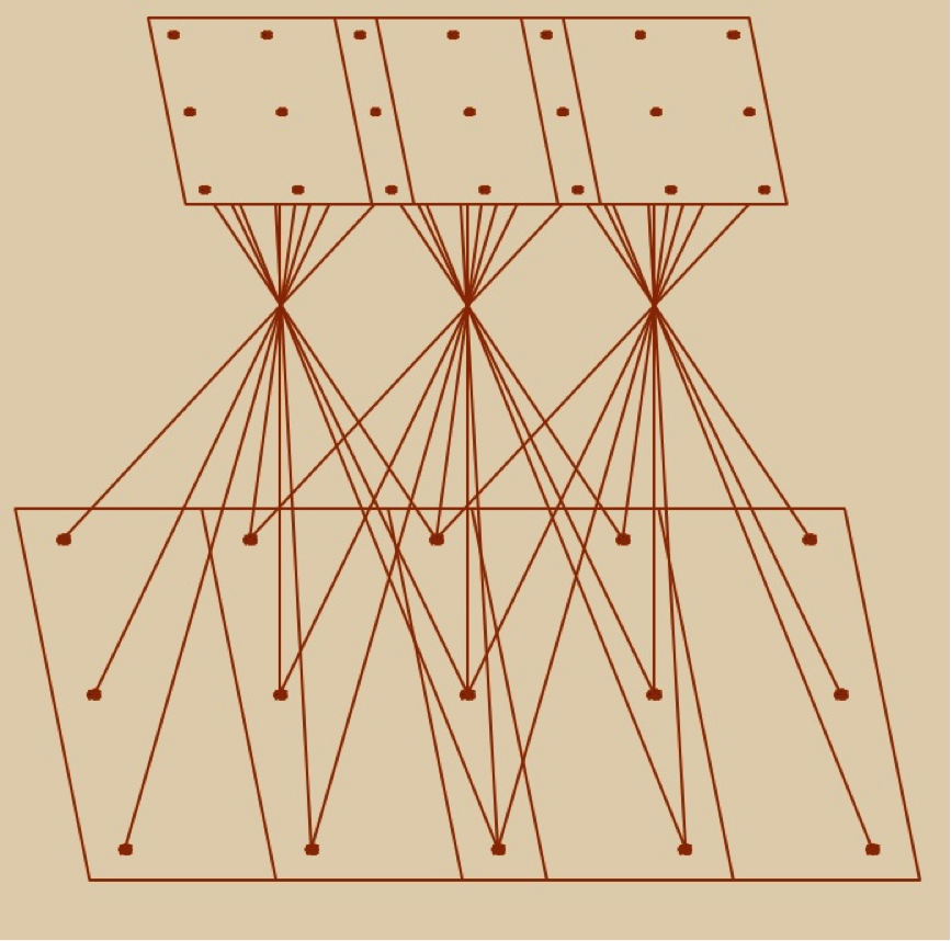
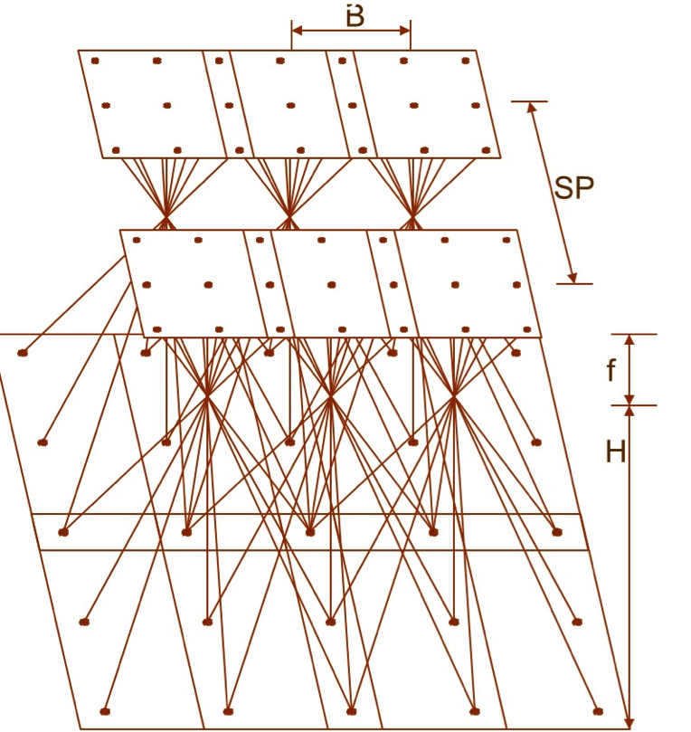
Figure 4.8 shows three overlapping squares with light rays entering the camera at the lens focal point. Successive overlapping images forms a strip of imagery we usually call "strip" or "flight line," therefore photogrammetric strip (Figure 4.8) is formed from multiple overlapping images along a flight line, while photogrammetric block (Figure 4.9) consists of multiple overlapping strips (or flight lines).

Flight Plan Design and Layout

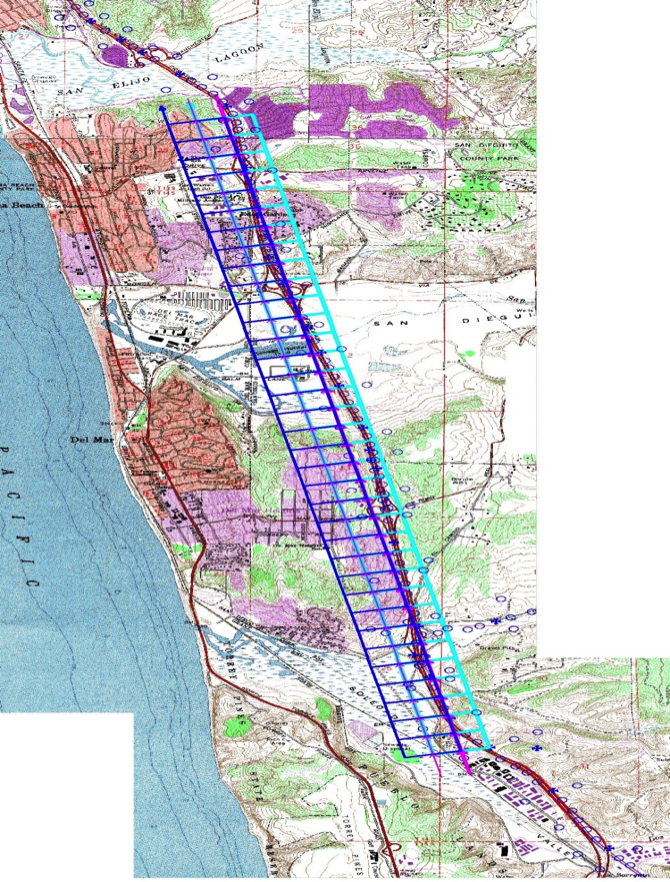
Once we compute the ground coverage of the image, as it was discussed in the "Geometry of Vertical Image" section, we can compute the number of flight lines and the number of images and draw them on the project map (Figure 4.10), aircraft speed, flying altitude, etc.

Before we start the computations of the flight lines and images numbers, I would like you to understand the following helpful hints:

• For a rectangularly shaped project, always use the smallest dimension of the project area to lay out your flight lines. This way it results in fewer flight lines and then less turns between flight lines (Figure 4.11). In Figure 4.11, the red lines with arrowheads represent flight lines or strips, while the black dash lines represent the project boundary.
  

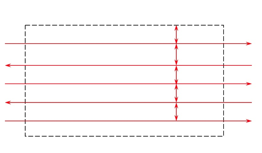  Figure 4.11 Correct flight lines orientation

  Source: Dr. Qassim Abdullah
• If you have a digital camera with a rectangular shape CCD array, always choose the largest dimension of the CCD array of the camera to be perpendicular to the flight direction (Figure 4.12). In Figure 4.12, the blue rectangles represent images as taken by a camera with rectangular CCD array. The wider dimension of the array is always configured to be perpendicular to the flight direction (which is the East-West direction for this figure).
  

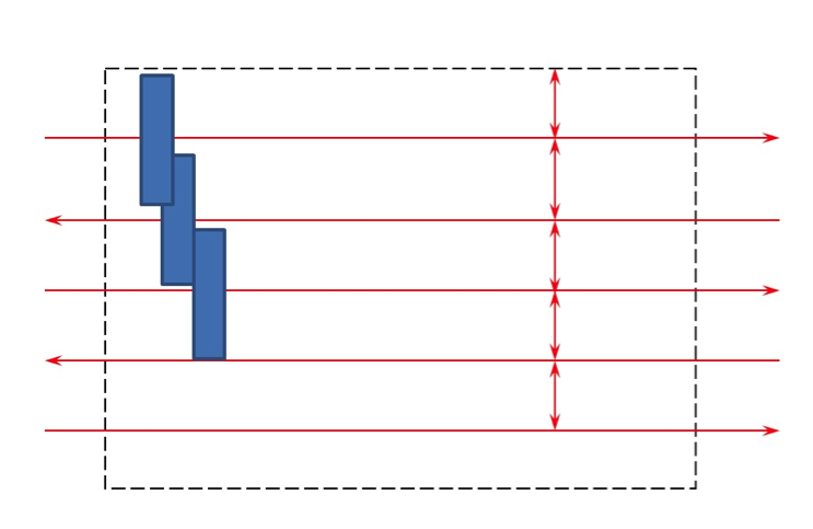  Figure 4.12 Correct camera orientation

  Source: Dr. Qassim Abdullah

Flight Lines Computations

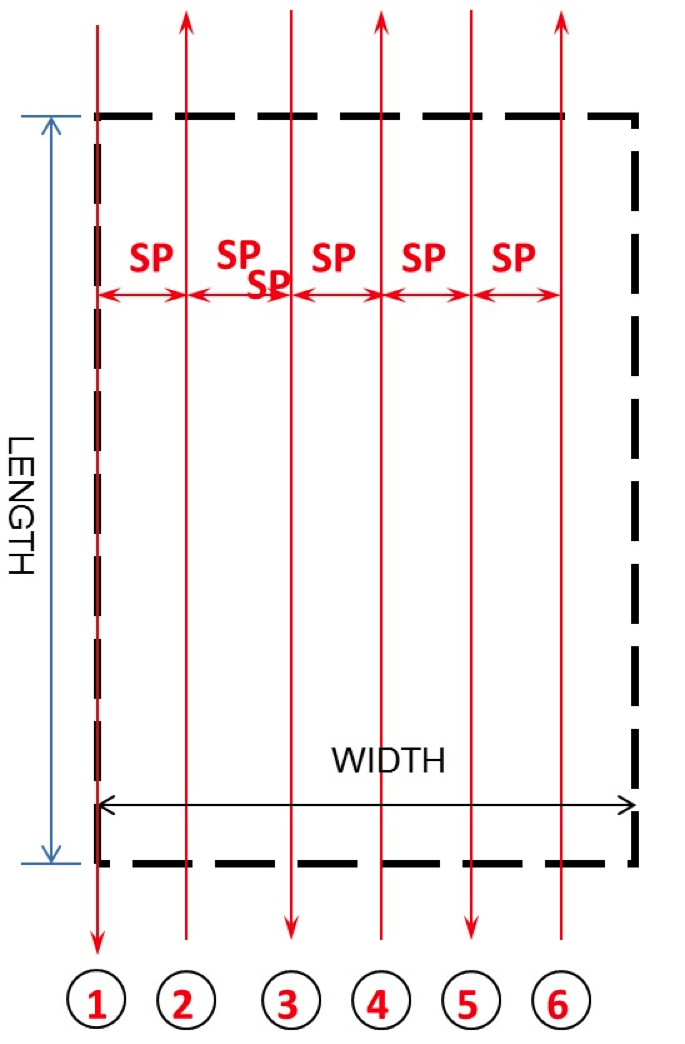
Now, let us start figuring out how many flight lines we need for the project area illustrated in Figure 4.13, to the right. Figure 4.13 shows rectangular project boundaries (in black dashed lines) with length equal LENGTH and width equal WIDTH that was designed to be flown with 6 flight lines (red lines with arrowheads). To figure out the number of flight lines needed to cover the project area, we will need to go through the following computations:

1. Compute the coverage on the ground of one image (along the width of the camera CCD array (or W)) as we discussed in section 4.3.
2. Compute the flight lines spacing as follows:
   Line spacing or distance between flight lines (SP) = Image coverage (W) x (100 – amount of side lap)/100.
3. Number of flight lines (NFL) = (WIDTH / SP) + 1.
4. Always round up the number of flight lines, i.e., 6.2 becomes 7.
5. Start the first flight line at the east or west boundary of the project.

In Figure 4.13, you may have noticed that the flight direction for each flight line alternates between North-to-South and South-to-North from one flight line to the adjacent one. Flying the project in this manner increases the aircraft fuel efficiency so the aircraft can stay longer up in the air.

Number of Images Computations

Once we determine the number of flight lines, we need to figure out how many images will cover the project area. To do so, we need to go through the following computations:

1. Compute the coverage on the ground of one image (along the height of the camera CCD array (or L)) as we discussed in section 4.3.
2. Compute the distance between two consecutive images, or what we call the “airbase,” B, as follows: Airbase or distance between two consecutive images (B) = Image coverage (H) x ((100 – amount of end lap)/100).
3. Number of images per flight line (NIM) = (LENGTH / B) + 1.
4. Always round up the number of images, i.e., 20.2 becomes 21.
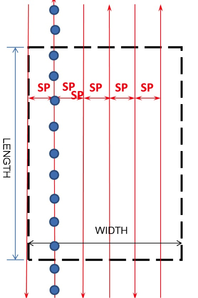
5. Add two images at the beginning of the flight line before entering the project area and two images upon exiting the project area Figure 4.14 (it is needed to insure continuous stereo coverage), i.e., total of additional 4 images for each flight line, or number of images per flight line = (LENGTH / B) + 1 + 4.
6. Total number of images for the project = NFL x NIM.

Figure 4.14 is the same as Figure 4.13 with added blue circles that represent photo centers of the designed images. The circles are only given to one flight line, and I will leave it to your imagination to fill all the flight lines with such circles.

Flight Altitude Computations

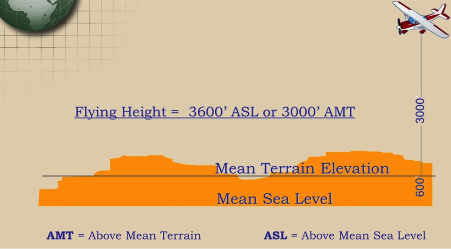
Flying altitude is the altitude above certain datum the UAS flies during data acquisition. The two main datum used are either the average (mean) ground elevation or the mean sea level. Figure 4.15 illustrates the relationship between the aircraft and the datum and how the two systems relate to each other. In Figure 4.15, we have an aircraft that is flying at 3000 feet above average (mean) ground elevation, represented by the blue horizontal line in the figure. We also have the mean terrain elevation (the blue horizontal line), situated at 600 feet above the mean sea level. Therefore, the flying altitude will be expressed in two ways, those are:

1. if we want to use the terrain as a reference, we will express it as Flying Altitude = 3000 feet above mean terrain or AMT;
2. if we use the sea level, we will express it as Flying Altitude = 3,600 feet above mean sea level (ASL or AMSL).

We now need to determine at what altitude the project should be flown. To do so, we go back to the camera internal geometry and scale as we discussed in section 4.3. Assume that the imagery to be acquired with a camera with lens focal length of f and with CCD size of b. We also know in advance what the imagery ground resolution or GSD should be. The flying altitude will be computed as follows:

$\text{scale = }\frac{\text{lens focal length (f)}}{\text{Flying height (H)}}=\frac{\text{distance }}{\text{ab}}$

OR

$\frac{f}{\text{flying}}=\frac{\mathrm{ab}}{\mathrm{AB}}$ from which, H can be determined.

$H=\frac{f•}{GSD}$

Here, we need to make sure that both f and b are converted to have the same linear unit, in which case the resulting altitude will be in the same linear unit of the GSD. If we assume the following values:

f = 50mm

ab = 0.010mm (or 10um)

GSD = 0.30 meter, the flying altitude will be:

$H=\frac{\text{50 mm}·\text{0.30 meter}}{\text{0.010 mm}}=1,500$ meters above ground level

Aircraft Speed and Image Collection

Controlling the aircraft speed is important for maintaining the necessary forward or end lap expected for the imagery. Fly the Aircraft too fast, and you end up with less forward lap than anticipated, while flying the aircraft too slowly results in too much overlap between successive images. Both situations are harmful to the anticipated products and/or the project budget. Little amount of overlap reduces the capability of using such imagery for stereo viewing and processing, while too much overlap results in too many unnecessary images that may affect the project budget negatively. In the previous subsections, we computed the airbase or the distance between two successive images along one flight line that satisfy the amount of end lap necessary for the project. Computing the time between exposures is a simple matter once the airbase is determined and the aircraft speed is decided upon.

Computing the time between two consecutive images

When the camera exposes an image, we need the aircraft to move a distance equal to the airbase before it exposes the next image. If we assume the aircraft speed is (v) therefore the time (t) between two consecutive images is calculated from the following equation:

$\text{Time (t) = }\frac{\text{Airbase (B)}}{\text{Aircraft Speed (v)}}$

For example, if we computed the airbase to be 1000 ft and we used aircraft with speed of 150 knots, the time between exposure is equal to:

$\begin{array}{l}\text{Time (t) = }\frac{\text{1000 ft}}{\text{150 knots}}\\ =\frac{\text{1000 ft}}{\text{150 knots }\cdot \text{1}\text{.15 miles}/\text{hour}}\\ =\frac{\text{1000 ft}}{\text{172}\text{.5 }\text{miles}/\text{hour}}\\ =\frac{\text{1000 ft}}{\text{172}\text{.5 }\text{miles}/\text{hour }\cdot \text{ 5280 }\text{ft}/\text{mile}}\\ \text{ = 0}\text{.0010979 hours}\\ \text{ = 3}\text{.95 sec}\end{array}$

Way Points

In the navigation world, way points are defined as “sets of coordinates that identify a point in physical space.” Close to this definition is the one used by mapping professionals, and that involves using sets of coordinates to locate the beginning point and the end point of each flight line. Way points are important for the pilot and camera operator to execute the flight plan. Way points in manned aircraft imagery acquisition are usually located a couple of miles outside the project boundary on both sides of the flight line (i.e., a couple of miles before approaching the project area and a couple of miles after exiting the project area or for UAS operations it would be a couple hundreds meters before approaching the project area and a couple hundreds meters after exiting the project area). The pilot uses way points to align the aircraft to the flight line before entering the project area. In UAS operation, a "Way Point" marks the beginning or the end of a flight line where the UAS either positions itself before starting taking pictures or it ends taking pictures on a certain flight line.

Example of Flight Plan Design and Layout

A project area is 20 miles long in the east-west directions and 13 miles in the north-south direction. The client asked for natural color (3 bands) vertical digital aerial imagery with a pixel resolution or GSD of 1 ft using a frame-based digital camera with a rectangular CCD array of 12,000 pixels across the flight direction (W) and 7,000 pixels along the flight direction (L) and a lens focal length of 100 mm. The array contains square CCDs with a dimension of 10 microns. The end lap and side lap are to be 60% and 30%, respectively. The imagery should be delivered in tiff file format with 8 bits (1 byte) per band or 24 bits per color three bands (RGB). Calculate:

1. the number of flight lines necessary to cover the project area if the flight direction was parallel to the east-west boundary of the project. Assume that the first flight line falls right on the southern boundary of the project;
2. the total number of digital photos (frames);
3. the ground coverage of each image in acres;
4. the storage requirements in gigabytes aboard the aircraft required for storing the imagery;
5. the flying altitude;
6. the time between two consecutive images if the aircraft speed was 150 knots.

Solution:

Looking into the project size (20x13 miles) and the one-foot GSD requirements, a mission planner should realize right away that image acquistion task for such project size and specifications can only be achieved using a manned aircraft.

The camera should be oriented so the longer dimension of the CCD array is perpendicular to the flight direction (see Figure 4.12).

1. $$ \begin{array}{l}{\text { Line spacing or distance between flight lines }(\mathrm{SP})=\text { tmage coverage }(\mathrm{W}) \times(100-\text { the amount of side }} \\ {\log ) / 100}\end{array} $$ $ =12,000 \text { pixels } x 1 \mathrm{ft} / \text { pixel } \mathrm{x}(100-30) / 100)=12,000 \times 0.70=8,400 \mathrm{ft} $ $$ \begin{array}{l}{\text { Number of flight lines }(\mathrm{NFL})=(\text { project WIDTH } / \mathrm{SP})+1=((13 \text { miles } \times 5,280 \mathrm{ft} / \mathrm{mile}) / 8,400 \mathrm{ft})+1=8.171} \\ {+1=9.171 \approx 10 \text { flight lines (with rounding up). }}\end{array} $$
2. $$ \begin{array}{l}{\text { Airbase or distance between two consecutive images }(\mathrm{B})=\text { Image coverage }(\mathrm{L}) \times((100-\text { amount of }} \\ {\text { end } \operatorname{lap}) / 100)=7000 \text { pixels } \times 1 \mathrm{ft} / \mathrm{pixel} \times(100-60) / 100 \mathrm{e} \text { ) }=7000 \mathrm{ft} \times 0.40=2,800 \mathrm{ft}}\end{array} $$ $$ \begin{array}{l}{\text { Number of images per flight line }=(\text { project } L E N G T H / B)+1+4=((20 \text { miles } x 5,280 \mathrm{ft} / \mathrm{mile}) / 2,800 \mathrm{ft})+} \\ {1+4=(105,600 / 2,800)+1+4=37.714+1+4=42.714 \approx 43 \text { images per flight line. }}\end{array} $$. $$ \begin{array}{l}{\text { Total number of images for the project }=10 \text { flight lines } \times 43 \text { images/fight line }=430 \text { images }} \\ {\text { (frames). }}\end{array} $$  
3. $$ \begin{array}{l}{\text { Ground coverage of each image }=\mathrm{W} \times \mathrm{L}=12,000 \text { pixels } \times 1 \mathrm{ft} \times 000 \text { pixels } \times 1 \mathrm{ft}=84,000,000.0 \mathrm{ft} 2=} \\ {84,000,000 \mathrm{ft} 2,143,560 \mathrm{ft} 2 / \mathrm{acre}=1,928.37 \text { acres. }}\end{array} $$  
4. The storage requirement for the RGB (color) images: Each pixel needs one byte per band, therefore each of the three (R,G,B) bands needs W x L x 1 byte/per pixel, or $$ 12,000 \text { pixels } \times 7,000 \text { pixels } \times 1 \text { byte/pixel }=84,000,000 \text { bytes }=84 \text { Mega bytes (Mb). } $$ $$ \begin{array}{l}{\text { Total storage requirement }=\text { Number of images } x \text { Number of bands } \times 84 \text { Mb/image }=430 \text { images } x} \\ {3 \times 84 \text { Mb/image }=108,360 \mathrm{Mb}=108.360 \text { Giga byte }(\mathrm{Gb}) .}\end{array} $$
5. $ \text { Flying Altitude } H=\frac{f \times G S D}{\text { ab }}=\frac{100 \mathrm{mm} \times 1 \mathrm{ft}}{0.010 \mathrm{mm}}=10,000 \mathrm{f} \text { above terrain. } $
6. Time between consectuive images $$ \begin{aligned} \text { Time }(\mathrm{t}) &=\frac{2,800 \mathrm{ft}}{150 \mathrm{knots}} \\ &=\frac{2,800 \mathrm{ft}}{150 \mathrm{knots} \cdot 1.15 \mathrm{miles} / \mathrm{hour}} \\ &=\frac{2,800 \mathrm{ft}}{172.5 \mathrm{miles} / \mathrm{hour}} \\ &=\frac{2,800 \mathrm{ft}}{172.5 \mathrm{miles} / \mathrm{hour} \cdot 5,280 \mathrm{ft} / \mathrm{mile}} \\ &=0.0030742 \mathrm{hours} \\ &=11.067 \mathrm{sec} \end{aligned} $$

Cost estimation and delivery schedule

Past experience with projects of a similar nature is essential in estimating cost and developing delivery schedule. In estimating cost, the following main categories of efforts and materials are considered:

• labor
• materials
• overhead
• profit

Once quantities are estimated as illustrated in the above steps, hours for each phase are established. Depending on the project deliverables requirements, the following labor items are considered when estimating costs:

• aerial photography
• ground control
• aerial triangulation
• stereo-plotting (# of models = # photos -1)
• map editing 
• ortho production
• lidar data cleaning

The table in Figure 4.16 provides an idea about the going market rates for geospatial products that can be used as guidelines when pricing a mapping project using manned aircraft operation and metric digital camera and lidar. The industry needs to come up with a comparable table based on Unmanned operations. There is no good pricing model established for UAS operation as the standards and produicts quality are widely varialble depending on who offers such services and whether it fall strictly under the "Professional Services" designation. 

Figure 4.16: Examples of the going market rates for geospatial data prices

Product	GSD ft	Price per sq mile	Comments
Ortho	0.5	$150-$200	Based on large projects
Ortho	1.0	$80-$100	Based on large projects
Ortho	2.0	$30-$60	Based on large projects
lidar	3.2	$100-$500	Depends on accuracy, terrain, and required details

Delivery Schedule

After the project hours are estimated, each phase of the project may be scheduled based on the following:

• number of instruments or workstations available
• number of trained personnel available
• amount of other work in progress and its status
• urgency of the project to the client

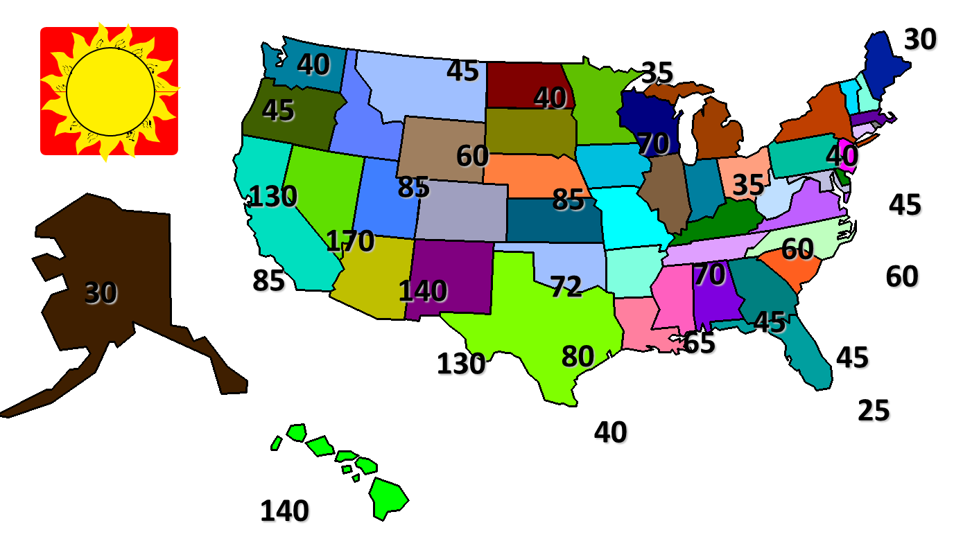
The schedule will also consider the constrains on the window of opportunity due to weather conditions. Figure 4.17 illustrates the number of days, per state/region, available annually for aerial imaging campaigns. Areas like the state of Maine have only 30 cloudless days per year that are suitable for aerial imaging activities.