Lesson 6: 3D Spatial Analysis
Overview
Overview
Importance of 3D Models in Spatial Analysis
In the previous lesson, you created a 3D map of the University Park campus. You learned how to symbolize layers based on procedural rule packages. In this lesson, you will learn two types of 3D spatial analysis. First, you will demonstrate the buildings that are affected in the case of a thunderstorm and a flash flood in State College. Second, you will learn how to do Sun Shadow analysis. It will give you a visual sense of how different sun positions will create various shadow volumes in different directions. It is a useful tool for building design and understanding the sun’s path in a given coordinate and also for figuring out the surface area that a building shades during a day.
Learning Outcomes
By the end of this lesson, you should be able to:
- Understand the importance of 3D models in certain geoprocessing analysis
- Present an example of 3D/spatial analysis
- Analyze the visibility of buildings and locations
- Calculate line of sights
- Calculate viewsheds
- Create layers
- Explore panning, zooming, and tilting
- Choose buildings and search for them
- Apply rules to extruded features
- Calculate, for example, a flood layer
- Share your work on Google Earth
Lesson Roadmap
| To Read |
|
|---|---|
| To Do |
|
Questions?
If you have any questions, please post them to our "General and Technical Questions" discussion (not e-mail). I will check that discussion forum daily to respond. While you are there, feel free to post your own responses if you, too, are able to help out a classmate.
Section One: Flood Analysis
Section One: Flood Analysis
Introduction
In this section, you will determine which areas of campus are more affected by flooding, by creating a raster layer representing accumulated water resulting from a thunderstorm. You will use the analytical 3D scene you created in the previous Lesson to visualize the flooding. In this study, you will use a FEMA flood map to find out how much of campus might be affected by the 1-percent annual chance flood, which is referred to as 100-year flood1. You will buffer the floodways around campus to present the flood plain and calculate the campus area affected by the 100-year flood. The floodway data is downloaded from FEMA flood map service center2. On flood plains, if you consider that water accumulation or the height of the water is a constant value, other factors that affect which areas are more affected by the flood are dependent on various factors. Examples of these factors are land elevation, surface material (pervious or impervious surfaces), vegetation coverage, and surface condition (saturated or dry). In this study, we only consider elevation as a factor. Therefore, you will extrude the flood data to see which buildings or trees are more affected.
For more information, refer to FEMA: Flood Zones [1]
1.1 Exploring Digital Elevation Model
1.1 Exploring Digital Elevation Model
-
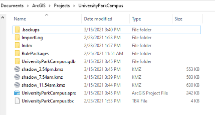
Download Lesson6.gdb [3] and unzip the file, then save it to the main project location.
(C:\Users\YOURUSER\Documents\ArcGIS\Projects\ UniversityParkCampus).
- Open UniversityParkCampus_Lesson6 Project in ArcGIS Pro.
- Click the Project tab. Select Save As.
 Credit: 2019 ArcGIS
 - In the Projects Folder (C:\Users\YOURUSER\Documents\ArcGIS\Projects\ UniversityParkCampus), Save Project as UniversityParkCampus_lesson6_Flood. This way you will create a new project for the first section of this lesson.
- Go back to the Map view.
- Turn on the Smoothed_DEM layer.
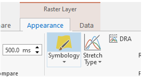
- To get a better idea of elevation around campus, click on the band color value under Smoothed_DEM. Then, on top ribbon, click on appearance and select symbology.
 Credit: ArcGIS, 2021
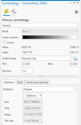 Credit: ArcGIS, 2021
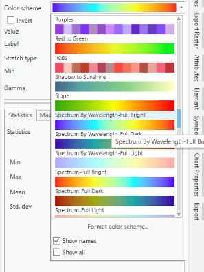
Change the color scheme to Spectrum by Wavelength-Full Bright. You can turn on Show names to see the names on top of each color scheme.
 Credit: ArcGIS, 2021
 -
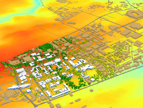
Go back to the Map_3D. Change the color scheme of Smoothed_DEM to Spectrum by Wavelength-Full Bright. Make sure that UP_Roof_Section and Building_Footprint layers are turned on. As you can see, the areas with higher elevations have warmer colors. It means that buildings located in the southern part of campus are more likely to be affected by flood, if we consider all the buildings in the same flood plain.
 Credit: ChronoPhronesis Lab
1.2 Adding Flood Map Layer and Understanding the Attributes
1.2 Adding Flood Map Layer and Understanding the Attributes
- Click the Map tab to return to your 2D map.
- Turn off Smoothed_DEM.
- Turn on UP_BUILDINGS.
- Click add data. and from Lesson6.gdb, add FLD_HAZ_FEMA layer. Make sure it is located below UP_BUILDINGS in the Contents Pane.
-
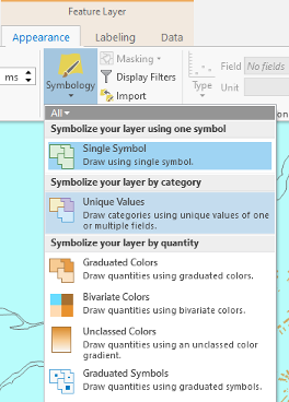
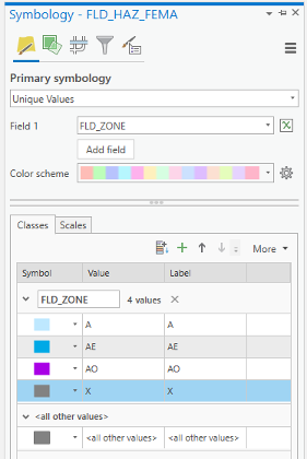
Click to modify symbology. Under the Appearance tab, select Symbology and choose Unique Values.
 Credit: ArcGIS, 2021
 -
As you have learned in previous lessons, symbolize your layers based on FLD_ZONE to have good visualization of various values. Remove the outline for values.
 Credit: 2019 ArcGIS
 -
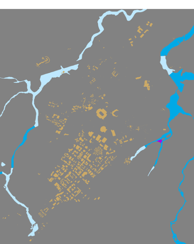
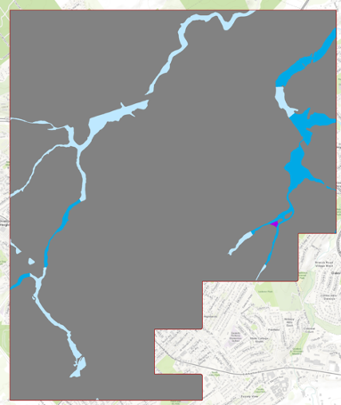
Zoom to UP_BUILDING layer. You should have a clear visualization of floodways with different categories.
 Credit: ChoroPhronesis Lab
Based on FEMA’s information3, categories A, AE, and AO are all 1-percent-annual-chance flood. A is determined using approximate methodologies. AE is created based on detailed methods. Finally, AO represents shallow flooding where average flood depths are between 1 to 3 feet. X represent areas that are not in a floodway. For this study, you are going to consider all three A, AE, and AO layers as one floodway category.
3FEMA: Flood Zones [1]
1.3 Extract Campus Area from FLD_HAZ_FEMA
1.3 Extract Campus Area from FLD_HAZ_FEMA
- Before creating flood plains, it would be better to select part of FLD_HAZ_FEMA layer that only contains the campus area.
-
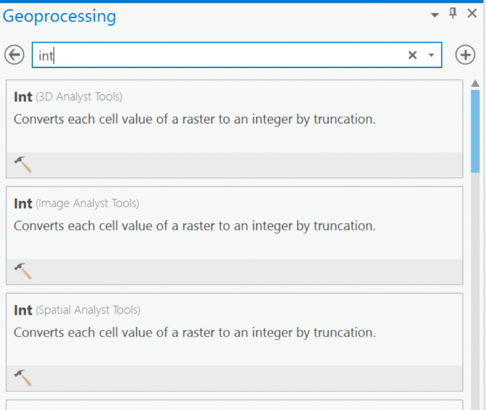
The best way to create a boundary is to use Smoothed_DEM layer as the extent of the campus area. To be able to create a polygon out of a raster, you will need a raster with integer values. The current raster values are float. On the ribbon, on the Analysis tab, click Tools under Geoprocessing and search Int. Click Int (Spatial Analysis). The input layer is Smoothed_DEM and rename the output raster to DEM_int. Click Run.
 Credit: 2019 ArcGIS
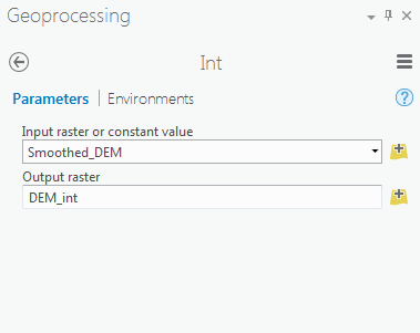 Credit: 2019 ArcGIS
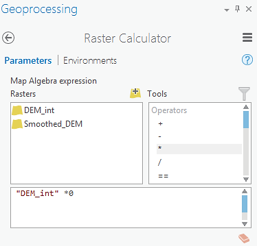
 - Go back to geoprocessing tool and search raster calculator. To create a polygon without values, you need a raster with pixel value of 0.
-
Select Raster Calculator (Spatial Analyst Tools). Using Raster calculator, multiply DEM_int by 0 to create a constant value raster.
 Credit: 2019 ArcGIS
Name the output raster as rasterzero. Click run. Now you have a raster with value of 0.
 Credit: ChoroPhronesis Lab
 -
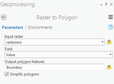
Go back to Geoprocessing Tools tab. Search or raster to polygon tool. Click Raster to Polygon (Conversion Tools). Convert rasterzero layer. Save the output polygon as Boundary. Click Run.
 Credit: 2019 ArcGIS
 -
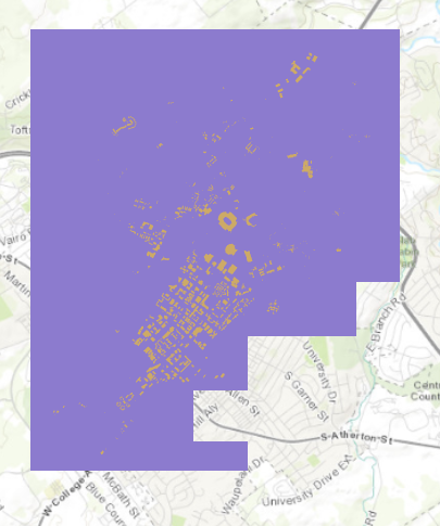
Remove rasterzero from Contents pane. You don’t need it anymore. Change the symbology of the Boundary layer to no fill, color with Tuscan Red, outline with the width of 2pt.
 Credit: ChoroPhronesis Lab
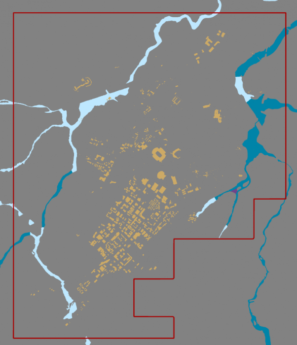
 - Now that you have created the campus boundary, you will clip FLD_HAZ_FEMA layer. Go back to Geoprocessing Tools. Search clip. Click Clip (Analysis Tools). The input layer is the flood layer from FEMA (FLD_HAZ_FEMA). The Clip Feature is Boundary. Rename the out feature class to FLD_HAZ_Campus. Click Run.
 Credit: ChoroPhronesis Lab
 -
Turn off FLD_HAZ_FEMA. And make sure that FLD_HAZ_Campus is located under UP_Buildiing. This will be the result.
 Credit: ChoroPhronesis Lab
1.4 Buffer the Floodways and Examine Potential Flood Extent
1.4 Buffer the Floodways and Examine Potential Flood Extent
For this study, you are going to consider all three A, AE, and AO layers as one floodway category.
-
On the ribbon, on the map tab, click select by attribute.
 Credit: 2016 ArcGIS
 -
Under expression, add the following clause to select all three floodway categories:
 Credit: ArcGIS, 2021
Click Apply, then OK. All three floodway categories will be selected.
 Credit: ChrorPhronesis Lab
Check Your Understanding
You have selected all the floodways on campus. Open the attribute table. Can you figure out how much the area of selected floodways are?
Click for the answer.15522969.81 square feet or 356.35 acre
This is how you can calculate the sum of the area:- Right-click on Shape_Area. Click Summarize.
- In the Geoprocessing tab, you can see the input and output tables. For Statistic Field, select Shape_Area. For the statistic Type select SUM. Click Run.
 Credit: 2016 ArcGIS
 -
In Geoprocessing Tools, search buffer. Click Buffer (Analysis Tools).
Note: When you have selected features in a layer, the analysis will run only on selected parts. -
The input feature is FLD_HAZ_Campus. Name the output feature class as Flood_Extent. For the distance consider 1000 feet. This distance is just an example to teach you how the analysis works. It does not mean that the flood plain in this area is truly 1000 feet.
Set Side Type as ‘Full’, meaning that the buffer will be from both sides of floodways. Click Run.
 Credit: 2016 ArcGIS
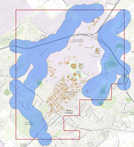 Credit: ChoroPhronesis Lab
 -
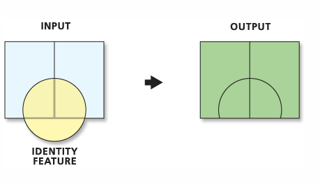
We are interested in the flood extent areas inside the boundary. The green areas are more affected than the rest of the campus. Now, you will create a polygon layer that has both areas: flood extent (1000 feet) and the rest of the campus. The proper tool to add the flood extent to the campus area is ‘Identity’. This tool computes geometric intersections of campus areas and flood plains. Those parts of campus overlapping with flood extent will get the attributes of identity features (flood extent).
 Credit: ArcGIS Pro [4]
 -
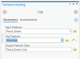
Before updating the flood zones of campus area, you need to clip the Flood_Extent, to extract areas inside the boundary. Go to Analysis tab, geoprocessing tools. Search Clip. Select Clip (Analysis Tools). Input feature is Flood_Extent. Clip Feature is Boundary. Name the output as Flood_Extent_Clip.
 Credit: ArcGIS, 2021
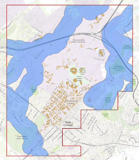 Credit: ChoroPhronesis Lab
 -
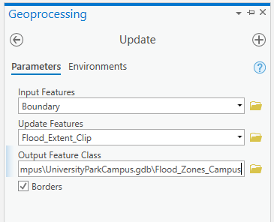
Turn off all layers. Go back to geoprocessing tools. Search update. Select Update (Analysis Tools). Input feature is Boundary, Update feature is Flood_Extent_Clip. Name the output feature class Flood_Zones_Campus. Click Run.
 Credit: ArcGIS, 2021
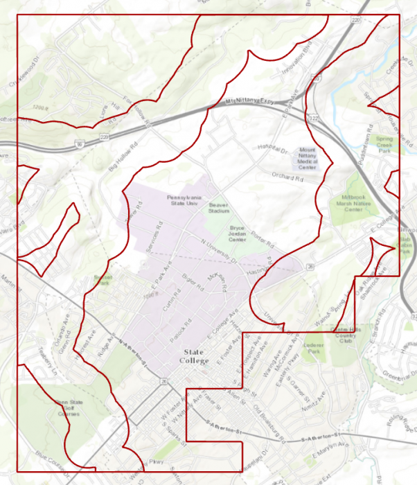 Credit: ChoroPhronesis Lab
 -
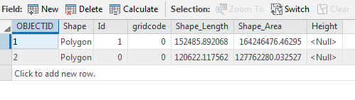
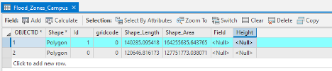
Right-click on Flood_Zones_Campus in Contents pane. Open Attribute Table. You can see there are two features in this layer with id categories 0 and 1. Select the row with id=0.
Check Your Understanding
What is the area of flood plain with higher risk (id=0) in acres?
Click for the answer.Approximately 2933.0 acres. Each square foot is approximately 2.295 acres.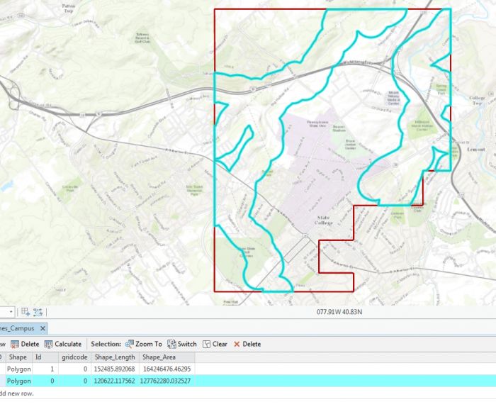 Credit: ChoroPhronesis Lab
The selected area is the 1000 feet extent from floodways and the rest is campus area with less flood risk in square feet.
- On the ribbon, on the Map tab, under selection category, click Clear.
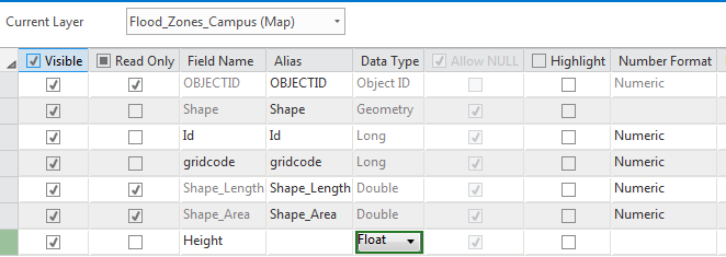
1.5 Add Height Attribute Data to the Flood_Zone_Campus Layer
1.5 Add Height Attribute Data to the Flood_Zone_Campus Layer
As you can see in the attribute table, the layer that you have created does not have any height information. You need water height information to extrude the layer properly in the 3D scene. Therefore, you will add a new attribute to the table and give it desired values.
- In the Contents pane, right-click Flood_Zones_Campus and choose Attribute Table.
-
At the top of the attribute table, click the Field Add button. The Fields view opens, where you will be able to edit parameters.
 Credit: ArcGIS, 2021
 -
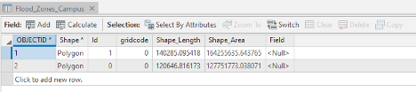
For the empty field at the bottom of the table, under Field Name, type Height. For Data Type, choose Float. Choosing Float over Integer allows you to have decimals.
 Credit: 2019 ArcGIS
 -
On the ribbon, on the Fields tab, click Save. The changes will be added to the table.
 Credit: ArcGIS, 2021
 -
Close the Fields view. Return to the attribute table.
 Credit: 2019 ArcGIS
 - Select the row with Id=0 by clicking the row.
-
On top of the attribute table click the Calculate field button.
 Credit: ArcGIS, 2021
 -
The input table is Flood_Zone_Campus. The field Name is Height. For the expression, you will consider 5 feet of flood for areas around the floodways. This number is for presentation purposes and is not accurate. Click OK.
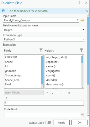 Credit: ArcGIS, 2021
 - Go back to the attribute table. Now you see the height value is 5.
- Click the second row with an id value of 1. Repeat the same calculate field step. This time Height =2 feet.
- Close the Calculate Field pane and the attribute table. Clear the selection.
1.6 Extrude the Flood_Zones_Campus Layer
1.6 Extrude the Flood_Zones_Campus Layer
- On the map tab, turn off the Topographic layer.
- Right- Click on Flood_Zone_Campus and select Copy.
- Click on Map_3D tab. Turn off Smoothed _DEM and WorldElevation3D/Terrain3D under Elevation surfaces/ Ground.
- Click on Map_3D in the contents pane and select paste. Flood_Zone_Campus will be added to your 2D_Layers.
-
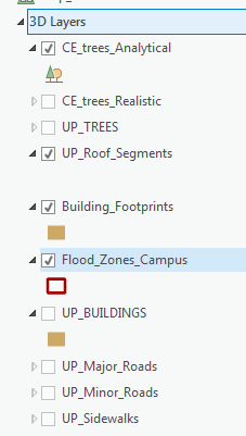
To add it to the 3D scene, in the Contents pane, drag Flood_Zones_Campus from 2D Layers to 3D layers. Placing it below Building_Footprints. Make sure the other 2D layers are off.
 Credit: 2016 ArcGIS
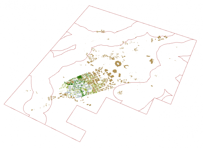 Credit: ChoroPhronesis Lab
 -
If you cannot see the layer, right-click on the layer and select properties. Click Elevation and make sure the Features are set as "on the ground".
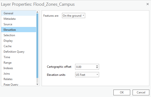 Credit: 2016 ArcGIS
 -
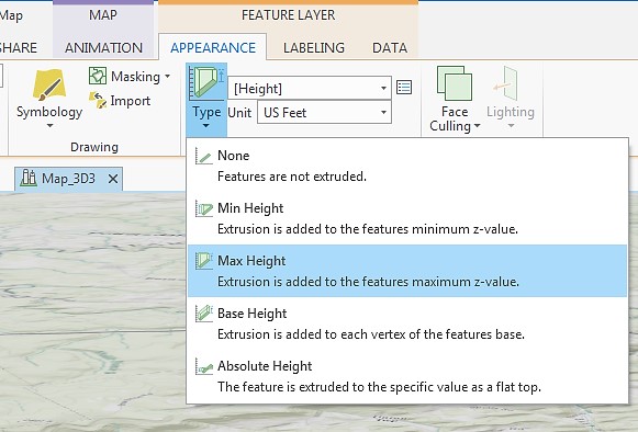
Click Flood_Zones_Campus. On the ribbon, click Appearance. Under Extrusion, choose Max Height as Extrusion Type. Select Height as the field of Extrusion. The Unit will be US Feet.
 Credit: 2016 ArcGIS
 -
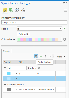
Click Flood_Zones_Campus. On the ribbon, click Appearance and from the Symbology drop-down menu choose Unique Values. In the Symbology pane, the value field is Id. Click Add all values. Change the color of id=0 as Apatite Blue with no border. The color for id=1 will be Sodalite Blue with no border.
 Credit: ArcGIS, 2021
 -
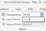
Again select the Flood_Zones_Campus. On the ribbon, click Appearance. On Effects group, change the transparency to 30 percent.
 Credit: ArcGIS, 2021
 -
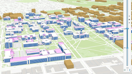
This will be the result:
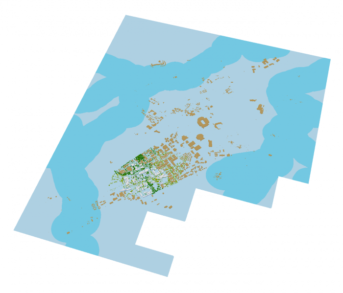 Credit: ChoroPhronesis Lab
 -
Using your mouse left click and V on the keyboard, navigate through the map. Zoom in to some buildings in different flood zones.
 Credit: ChoroPhronesis Lab
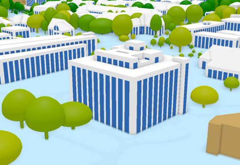 Credit: ChoroPhronesis Lab
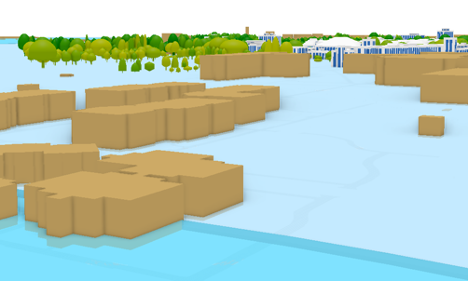
You can see how less Walker building is flooded compared to peripheral buildings on campus. Changing the height information flood elevation, you can have different results. If you are curious to see how the visualization changes, change the attribute values of Height field in the attribute table.
- Make a Screenshot of OldMain in which the level of flooding can be seen. Paste your screenshot into Word and label it Task 1.
- Save the Project.
Section Two: Sun Shadow Volume Analysis
Introduction
Section Two: Sun Shadow Volume Analysis
Introduction
Shadow analysis is a tool that allows you to analyze daylight conditions by giving a certain date and time. It can be hourly analysis between sunrise and sunset or the changes in shadows at a certain time during different dates. It is a useful tool for building design and understanding the sun’s path in a given coordinate. Assume that you are a designer and you would like to design a high-performance building that its source of energy is solar. Also, the sun position and movement across your site play an important role in your design to benefit from the daylighting.
The most important questions would be how much does a building shade the surrounding area and how much does the surrounding area, such as buildings and trees, shade a building? It is obvious that trees’ shadows are desirable in summer and very important in cooling the environment, whereas in the winter the important factor in the environment is the shade created by buildings.
In this section, you will carry out the sun shadow analysis from sunrise to sunset in winter (January 1st, 2021). If you are interested you can carry out another analysis for summer (July 1st, 2021) to compare the results. Creating the shadow volumes, you will learn how to animate the shadow volumes that you have created.
2.1 Understanding 3D Features
2.1 Understanding 3D Features
- Open UniversityParkCampus_Lesson6 Project in ArcGIS Pro.
-
Click the Project tab. Select Save As.
 Credit: 2016 ArcGIS
 - In the Projects Folder (C:\Users\YOURUSER\Documents\ArcGIS\Projects\ UniversityParkCampus), Save Project as UniversityParkCampus_Lesson6_Shadow.
- Go back to the Map view.
-
Make sure the following layers are checked in the 3D Layers Content Pane: Up_Roof_Segments, Building_Footprints., and Topography.
Note: What you have created in Lesson 5 as a 3D building, is an extrusion from attribute. It means that you extruded a 2D polygon based on a ‘Z’ attribute you extracted from LiDAR Data or DSM or any other sources. Having an extruded building, does not make your features with 3D geometry. It is just a 3D visualization of your 2D data. For many 3D spatial Analysis, you need 3D features or Multipatch features.
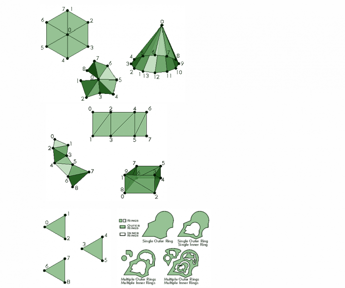
3D features are features with 3D geometry. 3D features can be displayed without the need to draping them over a surface like DEM. They already have Z information in their geometry. In the image below you can see how 2D features (Crème color) are dependent on a surface for display in a 3D scene, whereas 3D features (Red color) have z information and are located in the elevation they belong to without extrusion.
 Credit: ChoroPhronesis Lab
Multipatch features are 3D objects that represent a collection of patches to present boundary (or outer surface) of a 3D feature. Multipatches can be 3D surfaces or 3D solids (volumes).
Also, the icon next to a multipatch feature is a 3D feature. The image below shows the multipatch icon. For now the only supported type of features for multipatch layers are polygons. Points and lines can be converted to 3D features but not multipatch features.
 Credit: 2016 ArcGIS
 - For ‘Sun Shadow Analysis’ you need multipatch features. Multipatch features for buildings are provided in Lesson6.gdb.
-
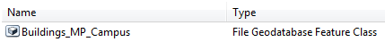
On the top ribbon, click Map and select Add Data. Locate Lesson6.gdb and select ‘Building_MP_Campus’.
Note: The reason that you will work on the smaller part of campus for this 3D spatial analysis is that your computer might not be able to handle bigger data. The multipatch layer for bigger areas of campus are also provided, in case you would like to carry on more analysis in your free time (Buildings_MP).
-
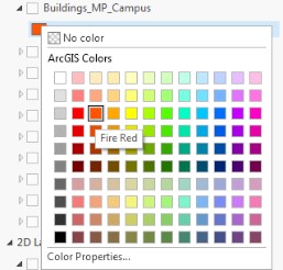
Right click on the symbol under layers to modify the color. Change the ‘Building_MP _Campus’ to Fire Red.
 Credit: 2016 ArcGIS
 -
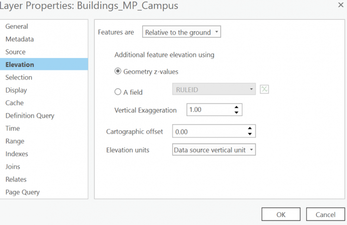
Right-click on Building_MP_Campus and select Properties. Select Elevation from the menu. Set the features are, Relative to the ground. Click Ok.
 Credit: 2019 ArcGIS
 -
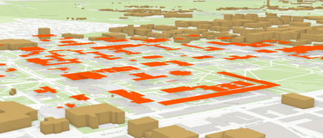
Uncheck UP_Roof_Segments. Now you can see what the multipatch surfaces look like. Navigate by holding down the scroll wheel or the V key and drag the pointer to tilt and rotate the scene.
 Credit: ChoroPhronesis Lab
Test Your Knowledge
- Uncheck this layer and check back the UP_Roof_Segments.
2.2 Sun Shadow Volume Analysis for January 1st
2.2 Sun Shadow Volume Analysis for January 1st
4 ArcGIS Pro [6]
5 ArcGIS Pro [6]
- On the top ribbon, click the Analysis tab and select tools. Search Sun Shadow.
-
Select Sun Shadow Volume (3D Analyst Tools).
 Credit: ArcGIS, 2021
 -
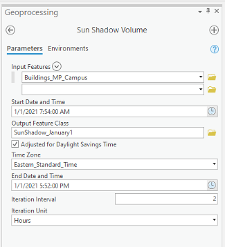
You will use the multipoint feature ‘Building_MP_Campus’ as an input. On January 1st, 2021 the sunrise is at 7:54 am and sunset is 5:52 pm. Set the start and end date as below. Pennsylvania is in the Eastern Standard Time zone. Change the Iteration Interval to 2 and Iteration Unit to Hours. Click Run.
 Credit: ArcGIS, 2021
 -
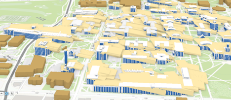
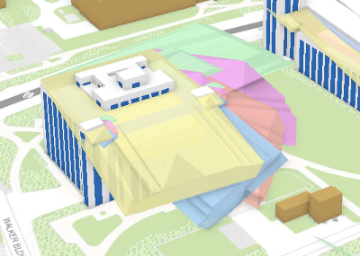
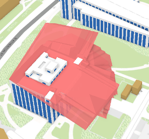
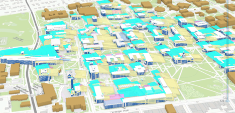
Turn on UP_Roof_Segment and turn off Building_Mp_Campus. Change the color of SunShadow_January to ‘Topaz Sand’. Right-click on the layer, select Properties. Click Elevation and make sure the features are relative to the ground. This is the result of your analysis.
 Credit: ChoroPhronesis Lab [7]
 - Open the attribute table and you will see the fields that are attributed. The fields are explained in detail on the ArcGIS Pro website. Here is the explanation for each field:
- SOURCE—Name of the feature class casting the shadow volume.
- SOURCE_ID—Unique ID of the feature casting the shadow volume.
- DATE_TIME—Local date and time used to calculate sun position.
- AZIMUTH—Angle in degrees between true north and the perpendicular projection of the sun's relative position down to the earth's horizon. Values range from 0 to 360.
- VERT_ANGLE—Angle in degrees between the earth's horizon and the sun's relative position where the horizon defines 0 degrees and 90 degrees is directly above.4
- Close the attribute table.
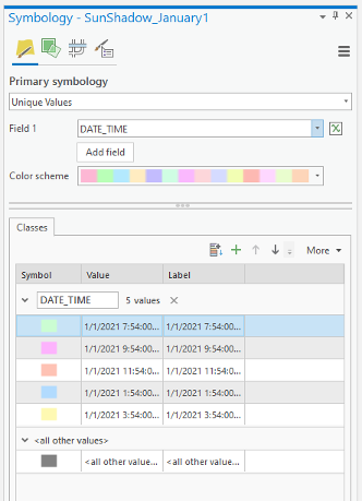
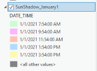
- To make sense of the results of the shadow volumes, you need to symbolize the layer based on the time of day (every 2 hours position of the sun in the local date). On the content pane, click on the symbology under SunShadow_January1.
-
On the top ribbon, under appearance, click Symbology. Select Unique Values.
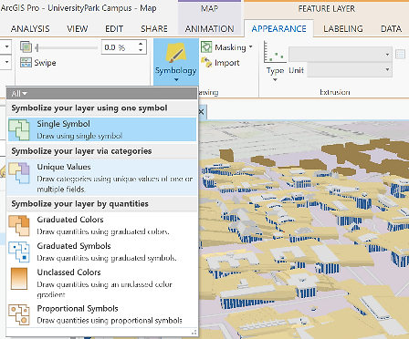 Credit: 2016 ArcGIS
 - On Symbology pane on the right side of ArcGIS Pro, select DATE_TIME as Value field.
-
Select set 3 for the color scheme.
 Credit: ArcGIS, 2021
 -
On the content pane or in the symbology pane you can explore the categories.
 Credit: ArcGIS, 2021
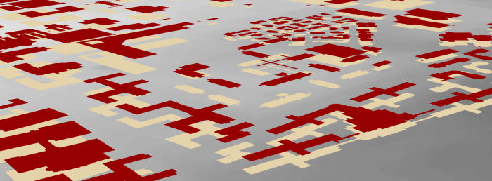
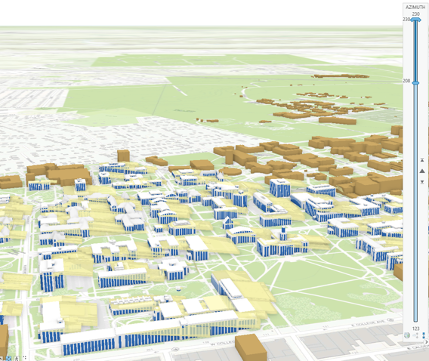
The first category is the shadow created by the sun at 7:54 am and the last one is the shadow created at 3:54 pm. Because of the overlaying layers, you cannot see each shadow clearly.
-
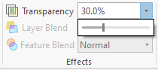
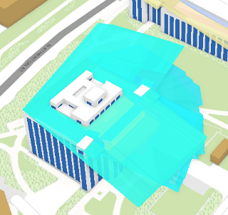
On the top ribbon, click appearance. In Effects Category, define Layer Transparency as 30%.
 Credit: ArcGIS, 2021
Making a Layer transparent, you can see different shadow volumes easier. However, there are more efficient ways to see your results.
ArcGIS Pro offers a few ways to show an area of interest for your data, including visibility ranges, definition queries, and range. To visualize your data as a dynamic range, you can use any layer, or set of layers, that contain numeric, non-date fields. Once you define the range properties for your layer, an interactive, on-screen slider is used to explore the data through a range you customized’.5
-
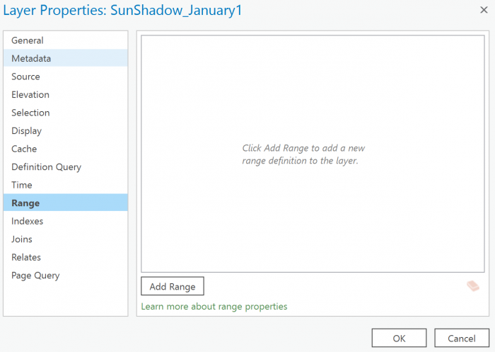
On the content pane, right-click on SunShadow_January1 layer and select properties. Click the Range Tab. Setting the range properties of the layer, you can explore the data interactively using a range slider.
 Credit: 2016 ArcGIS
 - To do so, you will choose a field by clicking add range. The range can be set by any numerical field. Therefore, you cannot choose DATE_TIME as a field for range.
-
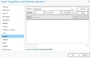
Click Add Range. Click the drop-down menu of Field. You will see that DATE_TIME is not in the list of fields that can be used because it is not a numerical field. You can select Azimuth. Set the extent from 120 to 236. Click Add. Click OK.
 Credit: ArcGIS, 2021
 -
Defining a range, you will be able to use a tool in ArcGIS Pro called Range Slider. This tool gives you the ability to filter overlapping content to make it more accessible and visible. You can see the Slider on the right side of your map.
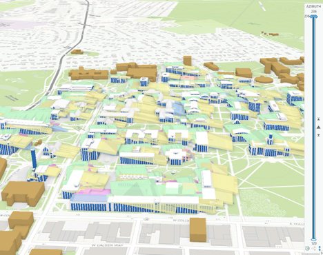 Credit: ChoroPhronesis Lab [7]
 -
To set the Slider, on the top ribbon, under Map, click Range. Under Full Extent choose Sun Shadow_January1. Make sure the min and max are set to 120 and 236.
 Credit: ArcGIS, 2021
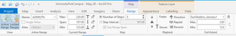
 - Playback defines the speed and direction of the range on the Range Slider to move.
- If you set the current range from 120 to 230. The span becomes 107. Set the number of steps to 5.
-
Make sure the active range is Azimuth, the same field you defined in layer properties.
Check Your Understanding
Take a look at your map. You can see the first visible range now is from 123 to 144. This azimuth range belongs to the first hour of the sunrise from 7:54 am to 9:54 am
Where is the shadow's direction of the first range? (From 7:54 am to 9:54 am)
Click for the answer.North West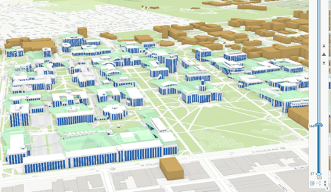 Credit: ChoroPhronesis Lab [7]
 - Click next on your slider and you can see the next result:
 Credit: ChoroPhronesis Lab [7]
This belongs to 8:35 am to 9:54 am. If you continue with the Range slider, you can see all 5 categories of time frames.
-
The last step shows you the changes in shadow volume and its direction towards the end of the day. The shadow moves from North West in the morning to the East towards the end of the day.
 Credit: ChoroPhronesis Lab [7]
 -
Instead of clicking next, you can play the slider and it will play ranges after each other with the pace you have chosen. The pace, from slower to faster can be defined on the top ribbon, Range tab.
 Credit: 2106 ArcGIS
 -
Here is the video of how the shadows of University Park Campus buildings move from sunrise to sunset on 01/01/2021.
Video: Sun Shadow January 1 2021 (00:37) This is video is not narrated. -
You have learned how to change symbology in Lesson 5. To make a more presentable animation of the shadow volumes, define the symbology of ‘SunShadow_January1’ using a gradual color change from lighter colors to darker colors. You need 5 gradual colors; for instance, you can choose a color ramp of Blue or Orange or Green or any other color you find appropriate.
Note: make sure to change the current range from 123 to 230 to see all shadow calcifications under the ‘SunShadow_January1’ layer.
- Make a Screenshot of Campus with gradual symbology of SunShadow_January1. Copy and paste the screenshot into your Word document and label it Task 2.
- Save your Project.
2.3 Calculate Ground Shadow Surface for Walker Building
2.3 Calculate Ground Shadow Surface for Walker Building
In this section, you are going to calculate the ground surface covered by shadow during the day for Walker building.
-
Change the current slider range to 123-230 to see all the shadow volumes.
 Credit: ChoroPhronesis Lab [8]
 - Zoom to Walker building displayed in the above image.
-
On the Content pane, click List by Selection.
 Credit: ArcGIS , 2021
 - Uncheck all layers. Make sure the only active (checked) layer is SunShadow_January1.
-
Go back to List by Drawing Order.
-
On the top ribbon, under the Map tab, click Select. Draw a rectangle on top of Walker building’s shadows to select them. Make sure not to select other buildings’ shadows.
 Credit: ChoroPhronesis Lab [8]
 -
Right-click on SunShadow_January1 layer. Click Data, Export Features.
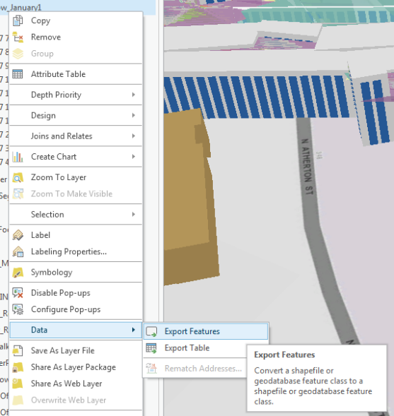 Credit: 2016 ArcGIS
 - The Export Features pane opens. Name the output feature ‘Shadows_Walker’. Click Run.
- On Content Pane, uncheck ‘SunShadow_January1’.
-
Click symbology under Appearance and change the color to the unique value. Change the color from white to another color.
 Credit: ChoroPhronesis Lab [8]
 - Now you have the shadow volumes for Walker Building in Multipatch format. To convert it to Polygons, on top ribbon, click Analysis and select Tools in Geoprocessing group.
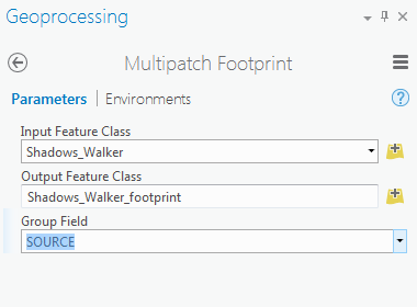
- Search Multipatch Footprints. Multipatch footprints create two-dimensional polygon footprints. Click the tool.
-
The Input Feature Class is Shadow_Walker. Name the output ‘Shadow_Walker_footprint’. To make one unique surface, you need to group your features based on a unique field. The “Source” field which is ‘Buildings_MP_Campus’ is a unique attribute that can group or dissolve all features together based on it. Click Run.
 Credit: 2016 ArcGIS
 -
You can see your layer in the 2D Layers list. Uncheck Shadow Walker from the 3D Layers.
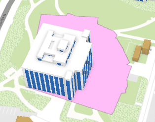 Credit: ChoroPhronesis Lab [8]
Check Your Understanding
What is the shadow area? Do you think it is an accurate shadow area?
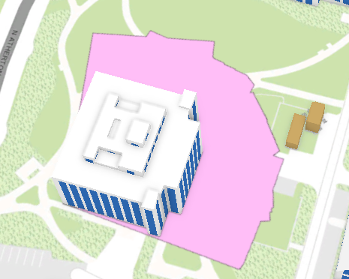
Click for answer.The shadow area of Walker building is around 50682.01 square feet. It is not a correct shadow area because at the beginning of this section, we asked you to calculate the ground shadow surface. However, the result of your shadow footprint contains the building itself. Although the building’s roof is covered by shadow during certain times of the day, we are only interested in ground surface.
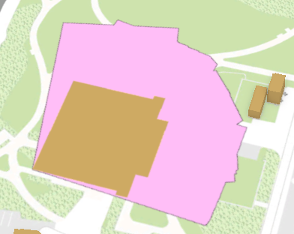
- To solve this issue, you should subtract Walker building’s footprint from the shadow surface.
-
Turn off Up_Roof_Segment. Drag UP_Buildings from 3D Layers to 2D Layers and turn it on. Make sure it is on top of Shadows_Walker_footprints.
 Credit: ChoroPhronesis Lab [8]
 -
On the top ribbon, click Analysis. Select Tools from Geoprocessing group. Search Erase.
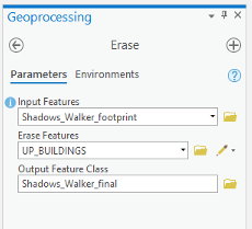 Credit: ArcGIS, 2021
 - Your input Features will be Shadow_Walker_footprints. Erase Features will be Up_Buildings. Name the Output Feature Class ‘Shadows_Walker_final’. Click Run.
- Uncheck Up_Buildings and Shadow_Walker_footprints.
- Now, you will see that the building footprint is extracted from the shadow.
-
Turn on Up_Roof_Segments.
 Credit: ChoroPhronesis Lab [8]Check Your Understanding
What is the area of Walker building Shadow now?
Click for the answer.35017.51 Square Feet
- Uncheck Shadows_Walker_final and turn on SunShadow_January1. Clear selection if necessary.
-
In this section, you have learned how to calculate the ground shadow surface for Walker building. In this assignment calculate ground shadow surface for the Nursing Sciences Building.
 Credit: ChoroPhronesis Lab [8]
 - Make a Screenshot of the ground shadow surface of Nursing Sciences Building. Copy and paste it into your Word document and label it Task 3.
- Make a Screenshot attribute of ground shadow surface of Nursing Sciences Building. We are interested in the total area of shadow surface. Copy and paste it into your Word document and label it Task 4.
- Save the project.
Section Three: Share Your Results on Google Earth
Section Three: Share Your Results on Google Earth
You would like to share the results of shadow volumes over the imagery. One way is to use Google Earth. It has both the imagery and 3D building models and is a good way to present your results.
Step 1: Download and install Google Earth
If you already have Google Earth skip this step. Otherwise, go through the following process:
- Open your web browser. Go to Google Earth [14].
- Click Earth Versions.
- Choose Google Earth Pro on Desktop.
- Click download Google Earth Pro.
- Install Google Earth Pro.
Step 2: Exporting to KML
KML (Keyhole Markup Language) is an XML based file format that is used in Earth browsers such as Google Earth and Google Maps. Consider you would like to share shadow surface in the morning, at noon and before sunset to demonstrate the shaded surface during the day. To do so, you will select the time of the day you are interested in and you will convert the Layer to KML.
- Open UniversityParkCampus_Lesson6_Shadow Project in ArcGIS Pro.
- On the top ribbon, click Select by Attributes.
 Credit: 2016 ArcGIS [15]
 - A Geoprocessing Pane on the right-hand side of the interface will open. Select SunShadow_January1. Add a clause that DATE_TIME value is equal to 8.36 am. Click Run.
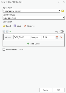 Credit: ArcGIS [15], 2021
 - You can see selected shadow volumes highlighted in blue.
 Credit: ArcGIS [15], 2021
 - On the top ribbon, click Analysis. Select Tools in the Geoprocessing group.
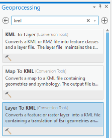
- In the Geoprocessing Pane on the right-hand side of the interface, search KML. Select Layer to KML (Conversion Tools).
 Credit: ArcGIS [15], 2021
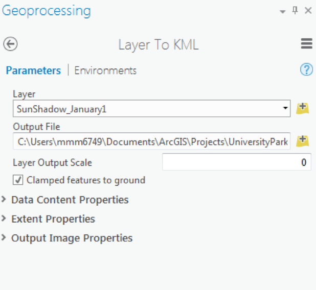
 - The input Layer will be SunShadow_January1. Only selected areas will be converted.
- Select the output folder and name the output Shadow_7.54am.
- Option Clamped features to the ground create shadow surface on the ground. Make sure it is checked. Click Run.
 Credit: 2016 ArcGIS [15]
 - This tool creates a KMZ file which might be confusing. We talked about KML and now the result is KMZ. A KMZ is a compressed KML. KMZ is smaller in size and easier to upload to the web. It contains the same data in KML format. You can unzip the file and see the KML inside the KMZ file.
 Credit: ArcGIS [15], 2021
 - Repeat this process for 11:54 am and 3.54 pm shadow volumes.
Step 3: Opening KMl/ KMZ in Google Earth
In this step, you will open three KMZ files you have created in Google Earth. Since Google Earth is free to use, then you can share your Google Earth file with anyone.
- Open Google Earth (Pro).
- Open a file explorer or windows explorer and navigate to the place you saved your KMZ files.
 Credit: 2021 Google Earth
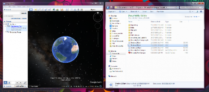
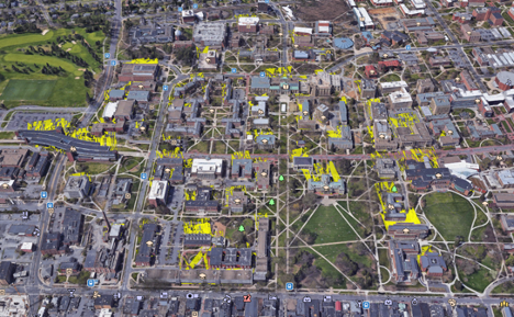
 - Move and resize the windows explorer and Google Earth, to see both at the same time next to each other. Drag and drop Shadow_7.54am into Google Earth.
 Credit: 2021 Google Earth
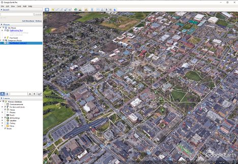
 - In the Google Earth interface, you will be directed to University Park Campus and you can see that Shadow_7.54am is added as a layer to Places Pane.
 Credit: 2021 Google Earth
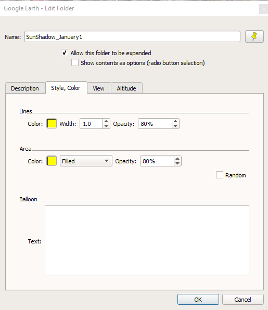
 - Right Click on Shadow_7.54am and click properties. Go to the Style, Color tab. Change both Lines and Area to yellow with 60% opacity. Click Ok.
 Credit: 2021 Google Earth
 - Use the navigation tool on the up right-hand of the interface to move around and rotate the map.
 Credit: 2021 Google Earth
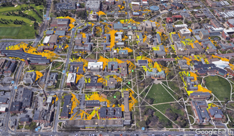
 - Drag and drop Layer Shadow_11.54am to Google Earth. Go to the Style, Color tab. Change both Lines and Area to orange with 80% opacity. Click Ok.
 Credit: 2016 Google Earth
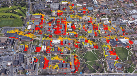
 - Drag and drop Layer Shadow_3.54m to Google Earth. Go to the Style, Color tab. Change both Lines and Area to red with 80% opacity. Click Ok.
 Credit: 2021 Google Earth
 - You can uncheck any of the shadow layers, just to see a shadow surface in a particular time. Zoom in to Old Main and see how the shadow surface changes during the day.
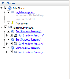
- On the Places Pane, right-click Temporary Places. Click Save Places As. Name the file "UniversityParkCampus_Shadow.kmz" and save it to your desired place. This is a file that you can share with anyone and they can promptly open it on Google Earth.
 Credit: 2021 Google Earth
Submit your file
Upload "UniversityParkCampus_Shadow.kmz" to Lesson 6 Assignment: Google Earth (2).
Guidelines and Grading Rubric
| Criteria | Full Credit | Half Credit | No Credit |
|---|---|---|---|
| Create a KMZ file | 4 pts | 2 pts | 0 pts |
| The KMZ file has all three shadows | 4 pts | 2 pts | 0 pts |
Tasks and Deliverables
Tasks and Deliverables
Assignment
This assignment has 4 parts, but if you followed the directions as you were working through this lesson, you should already have most of the first part done.
Part 1: Submit Your Deliverables to Lesson 6 Assignment: 3D Spatial Analysis
If you haven't already submitted your deliverable for this part, please do it now. You need to turn in all four of them to receive full credit. You can paste your screenshots into one file, or zip all of the PDFs and upload that. Make sure you label all of your tasks as shown below.
- Task 1: Screenshot of flooded Old Main (End of Section 1).
- Task 2: Screenshot of Campus with gradual symbology of SunShadow_January1 (End of Section 2.2)
- Task 3: Screenshot of ground shadow surface of Nursing Sciences Building (End of Section 2.3)
- Task 4: Screenshot of attributes of ground shadow surface of Nursing Sciences Building (End of Section 2.3)
Grading Rubric Criteria Full Credit No Credit Possible Points Task 1: Screenshot of flooded Old Main 4 pts 0 pts 4 pts Task 2: Screenshot of Campus with gradual symbology of SunShadow_January1 2 pts 0 pts 2 pts Task 3: Screenshot of ground shadow surface of Nursing Sciences Building 2 pts 0 pts 2 pts Task 4: Screenshot of attributes of ground shadow surface of Nursing Sciences Building 2 pts 0 pts 2 pts Total Points: 10
Part 2: Participate in a Discussion
Please reflect on your 3D spatial analysis experience, using ArcGIS Pro; anything you learned or any problems that you faced while doing your assignment as well as anything that you explored on your own and added to your 3D spatial analysis experience.
Instructions
Please use Lesson 6 Discussion (Reflection) to post your response to reflect on the options provided above and reply to at least two of your peer's contributions.
Please remember that active participation is part of your grade for the course.
Due Dates
Your post is due Saturday to give your peers time to comment. All comments are due by Tuesday at 11:59 p.m.
Part 3: Submit Your Deliverable to Lesson 6 Assignment: Google Earth
Instructions
Upload "UniversityParkCampus_Shadow.kmz" to the Lesson 6 Assignment: Google Earth.
Due Dates
Please upload your assignment by Tuesday at 11:59 p.m.
| Criteria | Full Credit | Half Credit | No Credit | Total |
|---|---|---|---|---|
| The KMZ file has all three shadows | 6 pts | 3 pts | 0 pts | 6 pts |
| Total points: 6 pts |
Part 4: Write a Reflection Paper
Instructions
Once you have posted your response to the discussion and read through your peers' comments, write a one-page paper reflecting on what you learned from working through the lesson and from the interactions with your peers in the Discussion.
Due Dates
Please upload your paper by Tuesday at 11:59 p.m.
Submitting Your Deliverables
Please submit your completed paper to the Lesson 6 Assignment: Reflection Paper.
Paper Grading Rubric
| Criteria | Full Credit | Half Credit | No Credit | Possible Points |
|---|---|---|---|---|
| Paper clearly communicates the student's experience developing the 3D spatial analysis in ArcGIS Pro. | 5 pts | 2.5 pts | 0 pts | 5 pts |
| The paper is well thought out, organized, contains evidence that student read and reflected on their peers' comments. | 3 pts | 1 pts | 0 pts | 3 pts |
| The document is grammatically correct, typo-free, and cited where necessary. | 2 pts | 1 pts | 0 pts | 2 pts |
| Total Points: 10 |
Summary and Tasks Reminder
Summary and Tasks Reminder
In this lesson, you have learned the importance of 3D data and 3D maps for spatial analysis. To explore various geoprocessing analysis, you have practiced two different methods to analyze flood and sun shadow analysis. In terms of 3D data, it is important to remember the difference between multipatch as 3D data and extruded 2D data. In the end, you experienced how to share your work on other platforms.
Reminder - Complete all of the Lesson 6 tasks!
You have reached the end of Lesson 6! Double-check the to-do list on the Lesson 6 Overview page to make sure you have completed all of the activities listed there before you begin Lesson 7.