3.1 Add and Explore Raster Data

In the previous section, you worked with feature data, data displayed as discrete objects, or features. While feature data is great for depicting buildings, roads, or trees, it is not the best way to depict elevation over a continuous surface. To do that, you'll use raster data, which can demonstrate a continuous surface. Raster data is composed of pixels, each with its own value. Although it looks different from feature data, you add it to the map in the same way.

1. If necessary, open the University Park Campus project in ArcGIS Pro.
2. In the Map tab, in the Layer group, click the Add Data button.
3. In the Add Data window, under My Computer, navigate to where you have saved the data. Double-click UP_BareEarth to add it to the map.
4. In the Contents pane, uncheck the boxes next to all layers, leaving only UP_BareEarth, UP_Buildings, and the basemap visible.
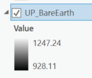
   The elevation unit is feet. Unlike the feature layer, which has shape geometry, raster layer use pixel matrices in which each pixel stores its own value. The layer resolution, the size of its pixels or cell size (x,y) is 2 by 2 square feet. The result, 4, means that each pixel represents an area of four square feet.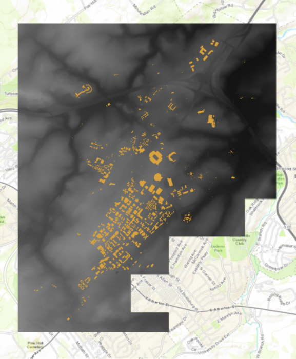
   

   Credit: ChoroPhronesis Lab [1]
5. In the Contents pane, click the arrow next to UP_BareEarth to view its symbology.
   

   Credit: 2020 ArcGIS [2]
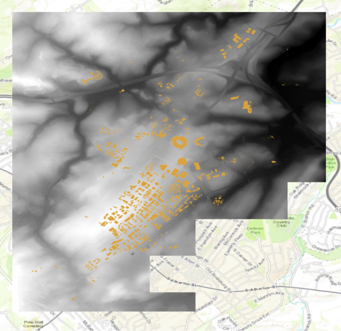
   Instead of a single symbol, this layer has a color scheme for different values. The values represent elevation in feet. The elevation ranges from about 825 feet above sea level (black) to about eighteen hundred feet above sea level (white).
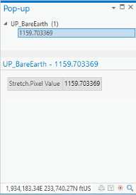
6. On the Map tab, in the Navigate group, click Explore. Click anywhere on the raster to open a pop-up window.
   

   Credit: 2021, ArcGIS [2]

   The pop-up shows the Pixel Value, which indicates the actual value of a pixel. In this raster, it shows the elevation. In the above image, the selected pixel has an elevation of about 1159 feet above sea level.

7. Close the pop-up.

3.2 Smoothing the DEM and Creating Contours

Before exploring the raster data in 3D, we need to smooth the elevation model, so the 3D model of campus fits the elevation model nicely. In order to monitor the level of smoothness of a DEM, creating contours can be helpful. A contour set built based on a raw digital elevation model (DEM) data can show minor variations and irregularities in the data. Creating a smooth contour set for topography is helpful in smoothing the data.

Note: the smooth grid should not be used for any analysis that requires raw DEM. For instance, building height cannot be extracted from a smoothed DEM.

1. At the top of the page, a ribbon is located. Click on the analysis tab.
   

   Credit: 2021, ArcGIS [2]
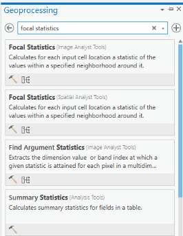
2. In the Geoprocessing group, click Tools.
3. In the Geoprocessing pane, search ‘Focal Statistics’.
   

   Credit: 2021, ArcGIS [2]
4. Select the Focal Statistics, which is located under Spatial Analyst Tool.

   The Focal Statistics tool will resample from the DEM and apply a search distance defined by cells or model distance.

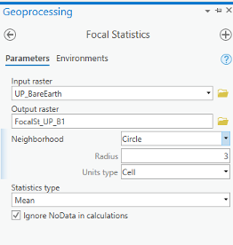
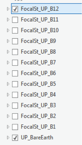
5. Choose UP_BareEarth as the input raster. Name the output raster so you can remember it! Every smoothed grid should be named and documented with information describing the smoothing process. The default name is FocalST_UP_B1. It means focal statistics phase 1.
6. Select Circle from the drop-down next to Neighborhood and set the smoothing Radius to 3. Leave all other default settings. Specify MEAN as the Statistics type.
   

   Credit: 2021, ArcGIS
7. Click Run on the bottom of the pane to create the first smoothed grid.
   

   Credit: ChoroPhronesis Lab [1]
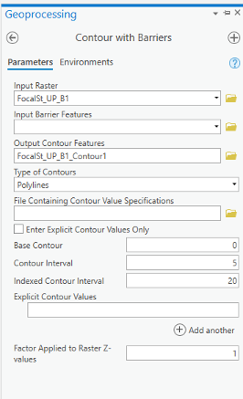
8. Contour lines can be created from this smoothed grid. Go back to the search bar in the Geoprocessing pane and search contour. Select contour with Barriers (Spatial Analyst Tool).
   

   Credit: 2021, ArcGIS [2]
9. Select FocalSt_UP_B1 as the Input raster and specify the output contour feature as FocalSt_UP_B1_Contour1. Types of Contour will be polyline. Set the Contour Interval to 5 feet and Indexed Contour Interval to 20 feet. Leave default values for other options. Click Run to create the contours.
   

   Credit: 2021, ArcGIS [2]
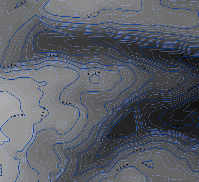
10. When the contours have been drawn, zoom in and inspect them. Notice that these lines are quite dense, especially when the entire model is viewed. Open the attribute table and verify that approximately 2,310 contour lines were created. These contours range in elevation from
    930 to 1245 feet.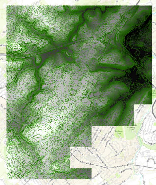
    

    Credit: ChoroPhronesis Lab [1]
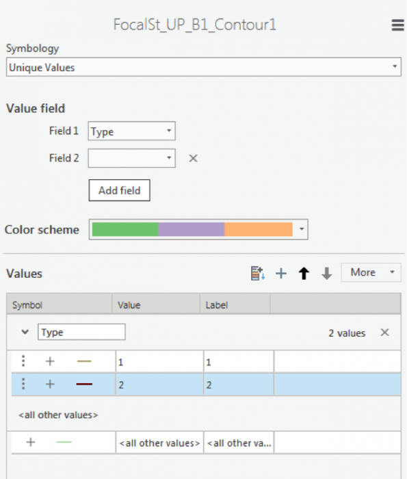
11. We can symbolize the indexed contour to have a better sense of elevation. Click the contour layer in the contents pane. Click the appearance tab. Under Symbology, select unique values. On the Symbology Pane symbolize based on value field “Type”. Type 1 are contours, which are every 5 feet and type 2 are barriers, which are every 10 feet.
    

    Credit: 2016 ArcGIS [2]
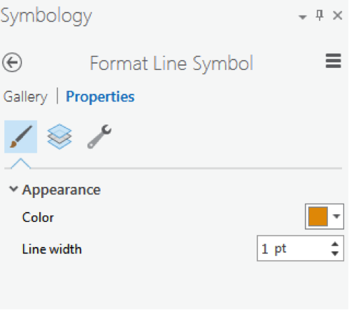
12. As you learned in the previous section, select symbology for each type. When you click format symbol, you can either choose Gallery (choose from preexisting styles) or choose Properties. We suggest properties.
    

    2016 ArcGIS [2]
    

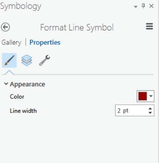    Credit: 2016 ArcGIS [2]

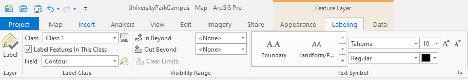
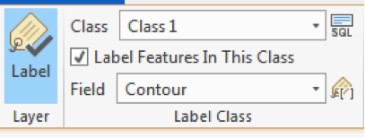
13. Click the contour layer in the contents pane. Make sure the symbol is highlighted by clicking on it. From the top ribbon, under Feature Layer, click Labeling. Under Label Class group, choose Contour for Field value. For class value click on the SQL button.

    

    Credit: 2021, ArcGIS [2]
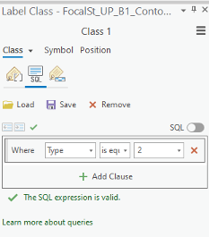
14. In Label Class pane, under SQL, click New Expression. Choose Type is equal to 2. With this selection, you will only label indexed contours. Click Apply.
    

    Credit: 2021, ArcGIS [2]
15. Go back to the labeling tab on top of your map. Choose font Corbel, size 12, bold, black.
16. Click Label button under Layer group.
    

    Credit: 2016 ArcGIS [2]
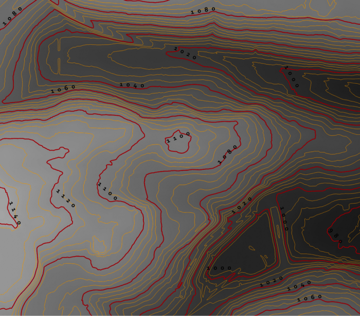
17. Your final result should look like this image.
    

    Credit: ChoroPhronesis Lab [1]
18. Keep this contour layer for comparison with the final result.
19. To have a smoother DEM, you have to repeat step 5 to 7 for a few times (Focal Statistics). Let’s say 12 times. Every time, you have to use the previous smoothed DEM. For instance, for the second round, you will use ‘FocalSt_UP_B1’ as an input. Keep the same naming system and options. Name the second output as FocalSt_UP_B2. You do not need to create contours for every smoothed layer. You will create another contour layer for the last output ‘FocalST_UP_B12’ to compare it with the first result.
    

    Credit: 2016 ArcGIS [2]
20. Now that you have the final DEM Layer (FocalST_UP_B12), Create Contour with Barriers for it. Repeat step 11 to 15. You can see how much smoother the new contours are. It means that we have a smooth DEM that is easier to work with.
    

    Credit: ChoroPhronesis Lab [1]
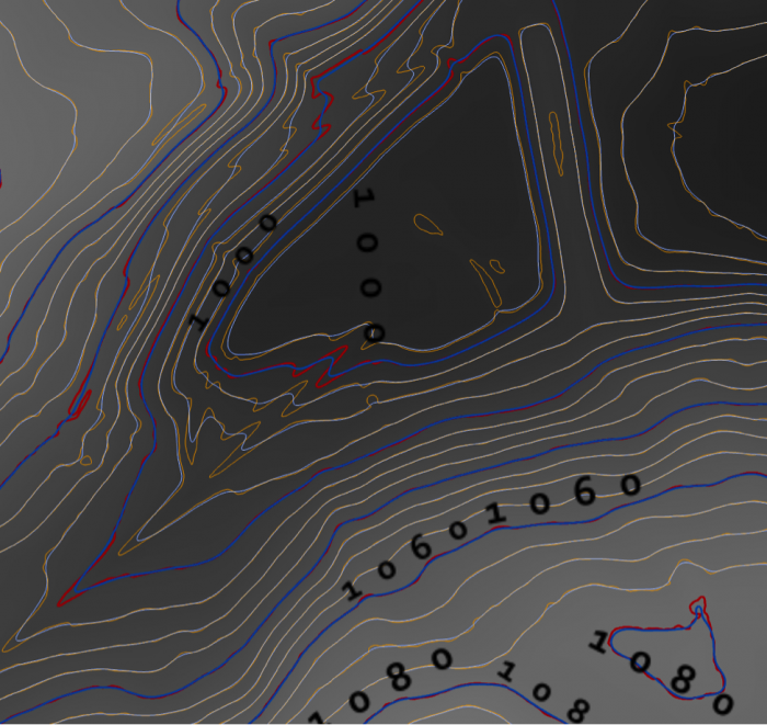
21. By choosing another color for the ‘FocalSt_UP_B1_Contour12’, you can compare the smoothness with the first created contour layer. You can choose light blue for the contours and dark blue for index contour. Repeat the labeling process to label your contours.
    

    Credit: ChoroPhronesis Lab [1]
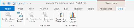
22. Select ‘FocalSt_UP_B1_Contour12’ in the Content Pane. From the top ribbon, choose Data, under Raster Layer. Click Export Data.
    

    Credit: 2021, ArcGIS [2]
23. As input Raster, choose ‘FocalSt_UP_B12'. Rename the output Raster to Smoothed_DEM. Click Run.
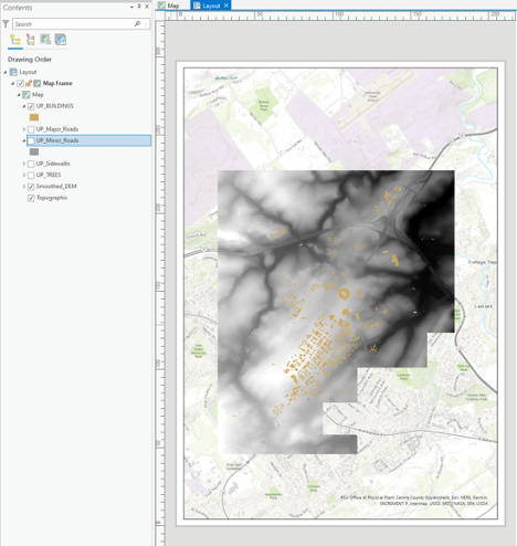
    You do not need the other raster/contour layers you created (from B1 to B12). You can remove them from your Contents pane. Also, remove UP_BareEarth.
24. For your final Assignment, you need a map of Smoothed_DEM and its full extent. Turn off all layers but Smoothed_DEM and Topographic. Zoom in or out, so that the DEM is in the center of your map.
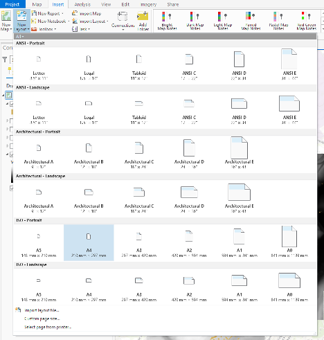
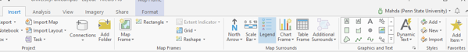
25. On top Ribbon, go to the Insert tab and add a new layout of A4 size. a layout page is opened.
    

    Credit: 2021, ArcGIS
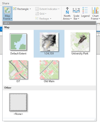
26. On Insert tab, click Map Frame and select the map option with Scale.
    

    Credit: 2021, ArcGIS
27. Draw the frame on the A4 paper layout that you would like the map to appear.
    

    Credit: 2021, ArcGIS
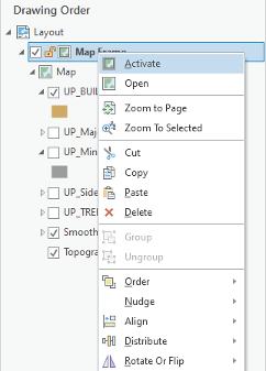
28. Under Layout, right-click on Map Frame and click Activate. You can zoom in and out until get the desired scale. Also, on the bottom of the page you can enter the desired scale. When finished, click Layout on top ribbon and Close Activation.
    

    Credit: 2021, ArcGIS [2]
    

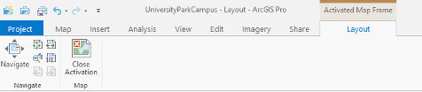    Credit: 2021, ArcGIS [2]
29. Under insert, click Legend on Map Surrounds.
    

    Credit: 2021, ArcGIS [2]
30. Draw the legend wherever you like on the Layout area. You can try to add a north arrow or scale bar if you are interested.
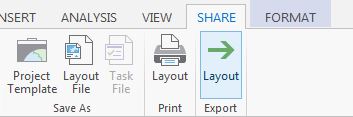
31. Click the Share tab. Under Print click Layout. Select Adobe PDF and Print the results. This is labeled as Task 2 on the Tasks and Deliverables.
    

    Credit: 2016 ArcGIS [2]