Section One: Flood Analysis

Introduction

In this section, you will determine which areas of campus are more affected by flooding, by creating a raster layer representing accumulated water resulting from a thunderstorm. You will use the analytical 3D scene you created in the previous Lesson to visualize the flooding. In this study, you will use a FEMA flood map to find out how much of campus might be affected by the 1-percent annual chance flood, which is referred to as 100-year flood¹. You will buffer the floodways around campus to present the flood plain and calculate the campus area affected by the 100-year flood. The floodway data is downloaded from FEMA flood map service center². On flood plains, if you consider that water accumulation or the height of the water is a constant value, other factors that affect which areas are more affected by the flood are dependent on various factors. Examples of these factors are land elevation, surface material (pervious or impervious surfaces), vegetation coverage, and surface condition (saturated or dry). In this study, we only consider elevation as a factor. Therefore, you will extrude the flood data to see which buildings or trees are more affected.

For more information, refer to FEMA: Flood Zones [1]

²FEMA Map Service Center (Borough of State College) [2]

1.1 Exploring Digital Elevation Model

Download Lesson6.gdb [3] and unzip the file, then save it to the main project location.

(C:\Users\YOURUSER\Documents\ArcGIS\Projects\ UniversityParkCampus).
Open UniversityParkCampus_Lesson6 Project in ArcGIS Pro.
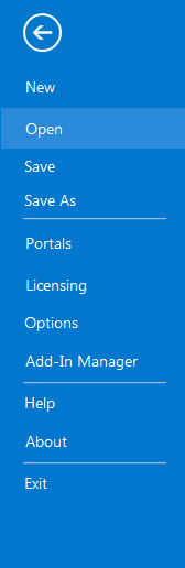
Click the Project tab. Select Save As.

Credit: 2019 ArcGIS
In the Projects Folder (C:\Users\YOURUSER\Documents\ArcGIS\Projects\ UniversityParkCampus), Save Project as UniversityParkCampus_lesson6_Flood. This way you will create a new project for the first section of this lesson.
Go back to the Map view.
Turn on the Smoothed_DEM layer.
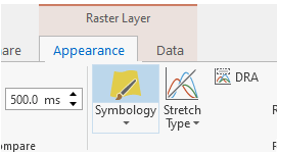
To get a better idea of elevation around campus, click on the band color value under Smoothed_DEM. Then, on top ribbon, click on appearance and select symbology.

Credit: ArcGIS, 2021

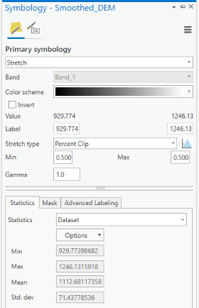Credit: ArcGIS, 2021

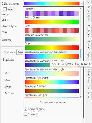
Change the color scheme to Spectrum by Wavelength-Full Bright. You can turn on Show names to see the names on top of each color scheme.

Credit: ArcGIS, 2021
Go back to the Map_3D. Change the color scheme of Smoothed_DEM to Spectrum by Wavelength-Full Bright. Make sure that UP_Roof_Section and Building_Footprint layers are turned on. As you can see, the areas with higher elevations have warmer colors. It means that buildings located in the southern part of campus are more likely to be affected by flood, if we consider all the buildings in the same flood plain.

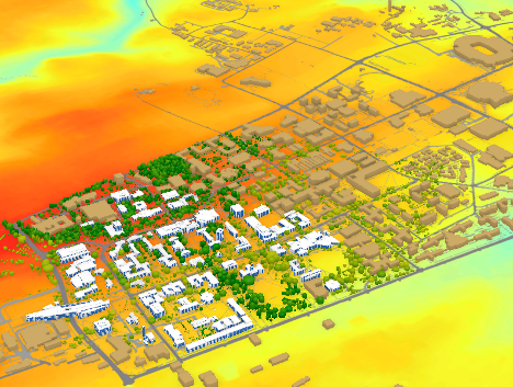Credit: ChronoPhronesis Lab

1.2 Adding Flood Map Layer and Understanding the Attributes

Click the Map tab to return to your 2D map.
Turn off Smoothed_DEM.
Turn on UP_BUILDINGS.
Click add data. and from Lesson6.gdb, add FLD_HAZ_FEMA layer. Make sure it is located below UP_BUILDINGS in the Contents Pane.
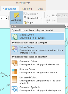
Click to modify symbology. Under the Appearance tab, select Symbology and choose Unique Values.

Credit: ArcGIS, 2021
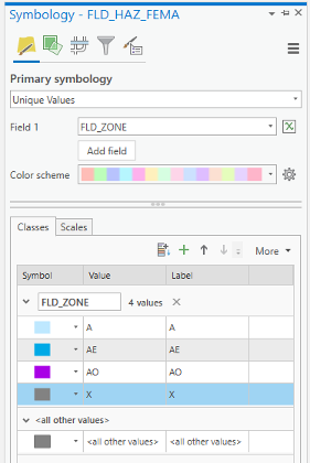
As you have learned in previous lessons, symbolize your layers based on FLD_ZONE to have good visualization of various values. Remove the outline for values.

Credit: 2019 ArcGIS
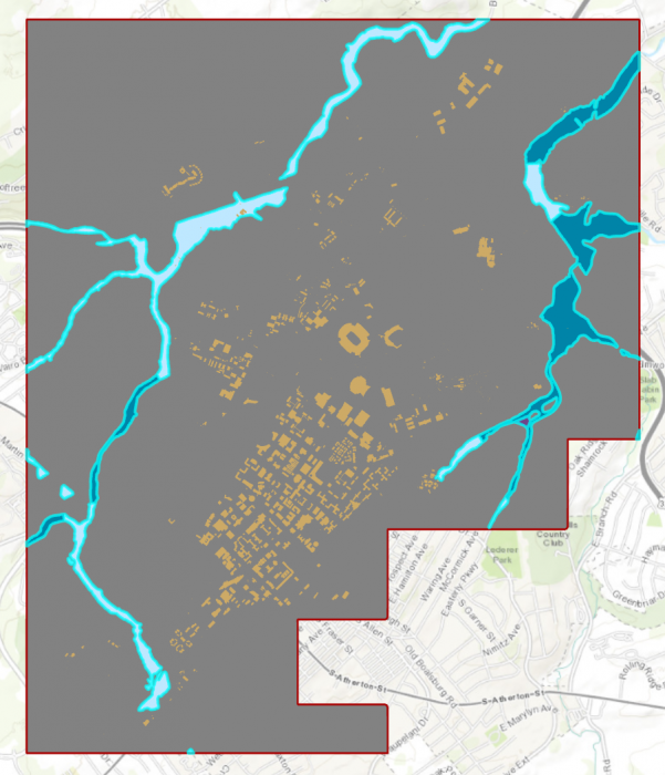
Zoom to UP_BUILDING layer. You should have a clear visualization of floodways with different categories.

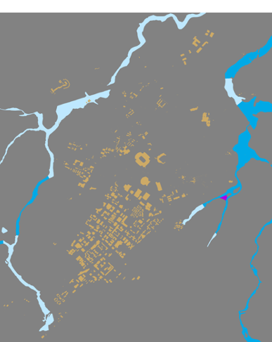Credit: ChoroPhronesis Lab

Based on FEMA’s information³, categories A, AE, and AO are all 1-percent-annual-chance flood. A is determined using approximate methodologies. AE is created based on detailed methods. Finally, AO represents shallow flooding where average flood depths are between 1 to 3 feet. X represent areas that are not in a floodway. For this study, you are going to consider all three A, AE, and AO layers as one floodway category.

³FEMA: Flood Zones [1]

1.3 Extract Campus Area from FLD_HAZ_FEMA

Before creating flood plains, it would be better to select part of FLD_HAZ_FEMA layer that only contains the campus area.
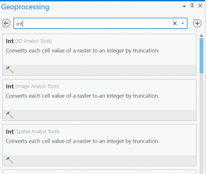
The best way to create a boundary is to use Smoothed_DEM layer as the extent of the campus area. To be able to create a polygon out of a raster, you will need a raster with integer values. The current raster values are float. On the ribbon, on the Analysis tab, click Tools under Geoprocessing and search Int. Click Int (Spatial Analysis). The input layer is Smoothed_DEM and rename the output raster to DEM_int. Click Run.

Credit: 2019 ArcGIS

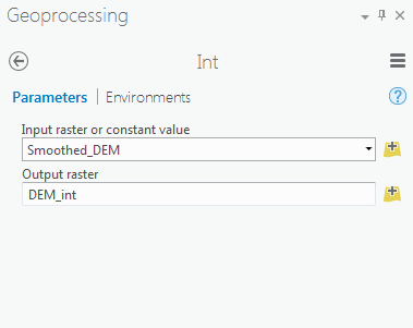Credit: 2019 ArcGIS
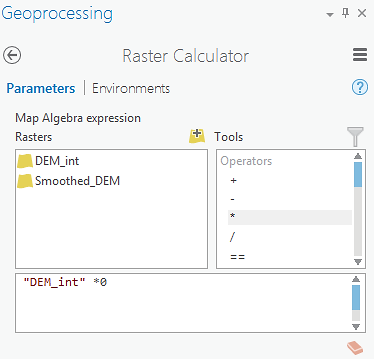
Go back to geoprocessing tool and search raster calculator. To create a polygon without values, you need a raster with pixel value of 0.
Select Raster Calculator (Spatial Analyst Tools). Using Raster calculator, multiply DEM_int by 0 to create a constant value raster.

Credit: 2019 ArcGIS

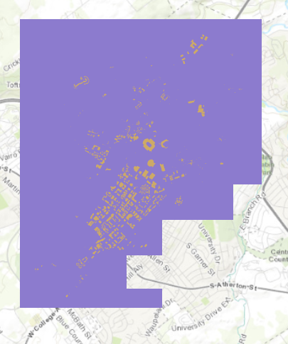
Name the output raster as rasterzero. Click run. Now you have a raster with value of 0.

Credit: ChoroPhronesis Lab
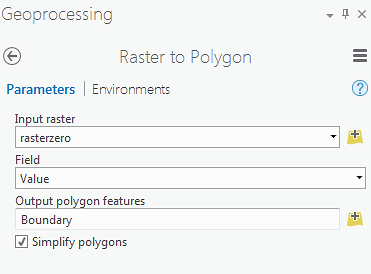
Go back to Geoprocessing Tools tab. Search or raster to polygon tool. Click Raster to Polygon (Conversion Tools). Convert rasterzero layer. Save the output polygon as Boundary. Click Run.

Credit: 2019 ArcGIS
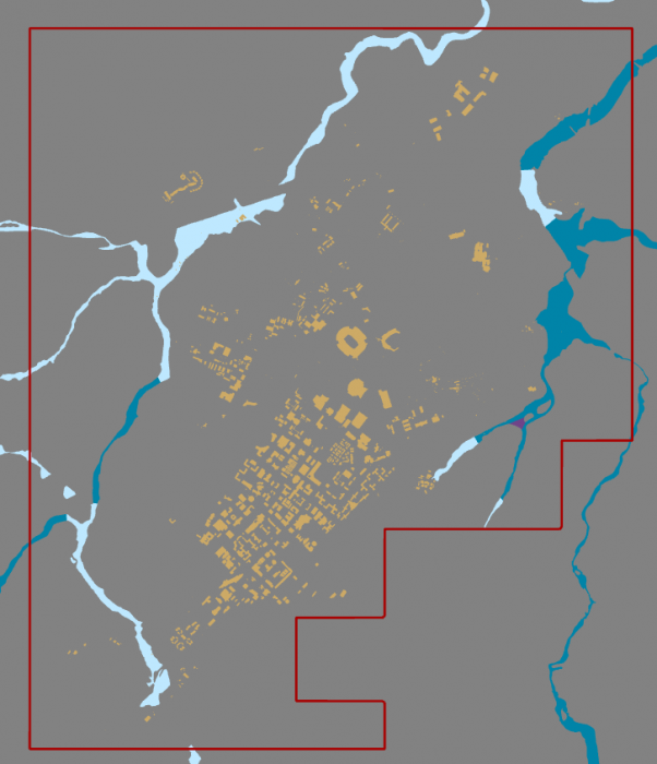
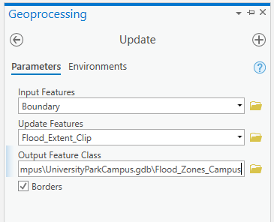
Remove rasterzero from Contents pane. You don’t need it anymore. Change the symbology of the Boundary layer to no fill, color with Tuscan Red, outline with the width of 2pt.

Credit: ChoroPhronesis Lab
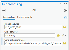
Now that you have created the campus boundary, you will clip FLD_HAZ_FEMA layer. Go back to Geoprocessing Tools. Search clip. Click Clip (Analysis Tools). The input layer is the flood layer from FEMA (FLD_HAZ_FEMA). The Clip Feature is Boundary. Rename the out feature class to FLD_HAZ_Campus. Click Run.

Credit: ChoroPhronesis Lab
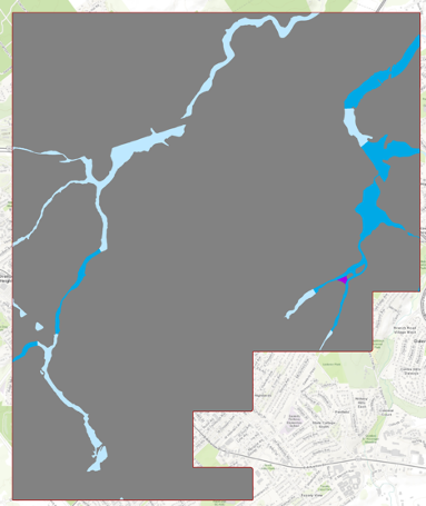
Turn off FLD_HAZ_FEMA. And make sure that FLD_HAZ_Campus is located under UP_Buildiing. This will be the result.

Credit: ChoroPhronesis Lab

1.4 Buffer the Floodways and Examine Potential Flood Extent

For this study, you are going to consider all three A, AE, and AO layers as one floodway category.

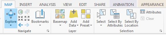
On the ribbon, on the map tab, click select by attribute.

Credit: 2016 ArcGIS
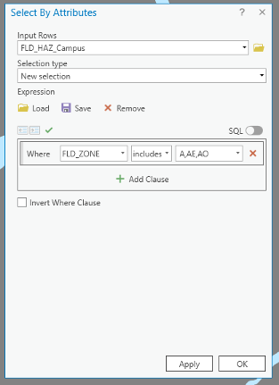
Under expression, add the following clause to select all three floodway categories:

Credit: ArcGIS, 2021

Click Apply, then OK. All three floodway categories will be selected.

Credit: ChrorPhronesis Lab
Check Your Understanding

You have selected all the floodways on campus. Open the attribute table. Can you figure out how much the area of selected floodways are?

Click for the answer.
15522969.81 square feet or 356.35 acre

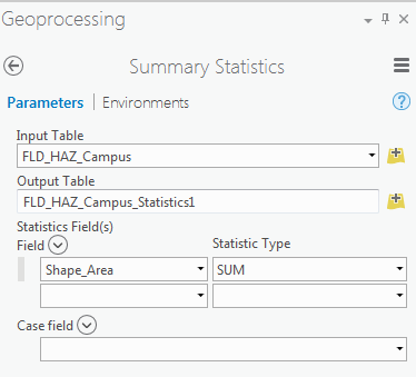
This is how you can calculate the sum of the area:
- Right-click on Shape_Area. Click Summarize.
- In the Geoprocessing tab, you can see the input and output tables. For Statistic Field, select Shape_Area. For the statistic Type select SUM. Click Run.
Credit: 2016 ArcGIS
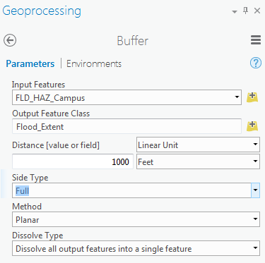
In Geoprocessing Tools, search buffer. Click Buffer (Analysis Tools).
Note: When you have selected features in a layer, the analysis will run only on selected parts.
The input feature is FLD_HAZ_Campus. Name the output feature class as Flood_Extent. For the distance consider 1000 feet. This distance is just an example to teach you how the analysis works. It does not mean that the flood plain in this area is truly 1000 feet.

Set Side Type as ‘Full’, meaning that the buffer will be from both sides of floodways. Click Run.

Credit: 2016 ArcGIS

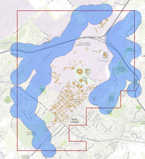Credit: ChoroPhronesis Lab
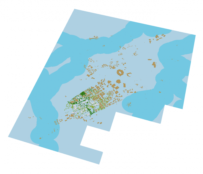
We are interested in the flood extent areas inside the boundary. The green areas are more affected than the rest of the campus. Now, you will create a polygon layer that has both areas: flood extent (1000 feet) and the rest of the campus. The proper tool to add the flood extent to the campus area is ‘Identity’. This tool computes geometric intersections of campus areas and flood plains. Those parts of campus overlapping with flood extent will get the attributes of identity features (flood extent).

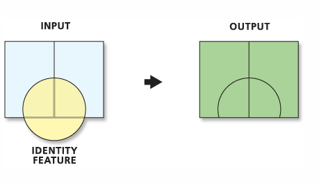Credit: ArcGIS Pro [4]
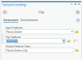
Before updating the flood zones of campus area, you need to clip the Flood_Extent, to extract areas inside the boundary. Go to Analysis tab, geoprocessing tools. Search Clip. Select Clip (Analysis Tools). Input feature is Flood_Extent. Clip Feature is Boundary. Name the output as Flood_Extent_Clip.

Credit: ArcGIS, 2021

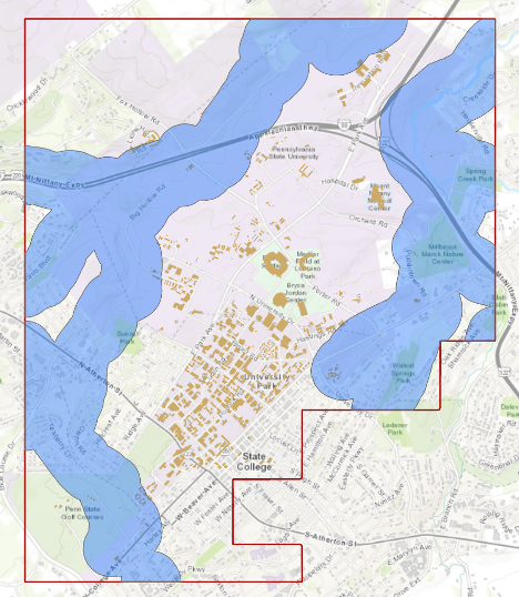Credit: ChoroPhronesis Lab
Turn off all layers. Go back to geoprocessing tools. Search update. Select Update (Analysis Tools). Input feature is Boundary, Update feature is Flood_Extent_Clip. Name the output feature class Flood_Zones_Campus. Click Run.

Credit: ArcGIS, 2021

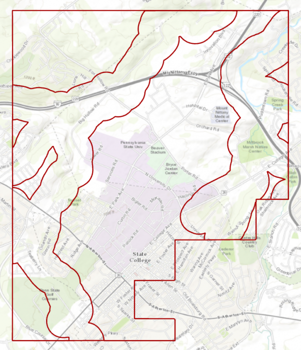Credit: ChoroPhronesis Lab
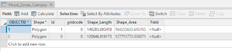
Right-click on Flood_Zones_Campus in Contents pane. Open Attribute Table. You can see there are two features in this layer with id categories 0 and 1. Select the row with id=0.

Check Your Understanding

What is the area of flood plain with higher risk (id=0) in acres?

Click for the answer.

Approximately 2933.0 acres. Each square foot is approximately 2.295 acres.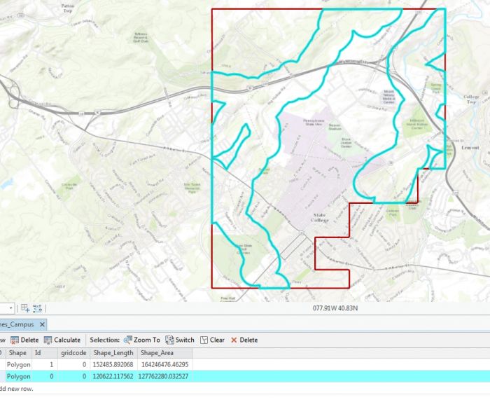

Credit: ChoroPhronesis Lab

The selected area is the 1000 feet extent from floodways and the rest is campus area with less flood risk in square feet.
On the ribbon, on the Map tab, under selection category, click Clear.

1.5 Add Height Attribute Data to the Flood_Zone_Campus Layer

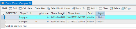
As you can see in the attribute table, the layer that you have created does not have any height information. You need water height information to extrude the layer properly in the 3D scene. Therefore, you will add a new attribute to the table and give it desired values.

In the Contents pane, right-click Flood_Zones_Campus and choose Attribute Table.
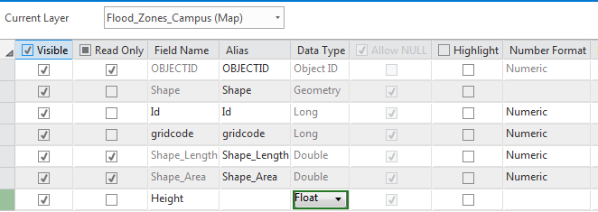
At the top of the attribute table, click the Field Add button. The Fields view opens, where you will be able to edit parameters.

Credit: ArcGIS, 2021
For the empty field at the bottom of the table, under Field Name, type Height. For Data Type, choose Float. Choosing Float over Integer allows you to have decimals.

Credit: 2019 ArcGIS
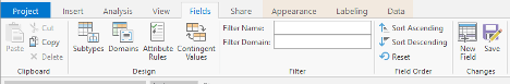
On the ribbon, on the Fields tab, click Save. The changes will be added to the table.

Credit: ArcGIS, 2021
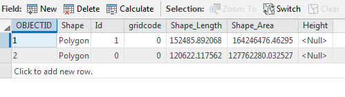
Close the Fields view. Return to the attribute table.

Credit: 2019 ArcGIS
Select the row with Id=0 by clicking the row.
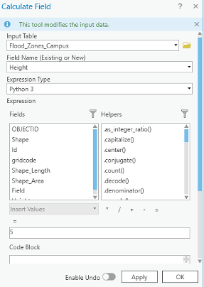
On top of the attribute table click the Calculate field button.

Credit: ArcGIS, 2021
The input table is Flood_Zone_Campus. The field Name is Height. For the expression, you will consider 5 feet of flood for areas around the floodways. This number is for presentation purposes and is not accurate. Click OK.

Credit: ArcGIS, 2021
Go back to the attribute table. Now you see the height value is 5.
Click the second row with an id value of 1. Repeat the same calculate field step. This time Height =2 feet.
Close the Calculate Field pane and the attribute table. Clear the selection.

1.6 Extrude the Flood_Zones_Campus Layer

On the map tab, turn off the Topographic layer.
Right- Click on Flood_Zone_Campus and select Copy.
Click on Map_3D tab. Turn off Smoothed _DEM and WorldElevation3D/Terrain3D under Elevation surfaces/ Ground.
Click on Map_3D in the contents pane and select paste. Flood_Zone_Campus will be added to your 2D_Layers.
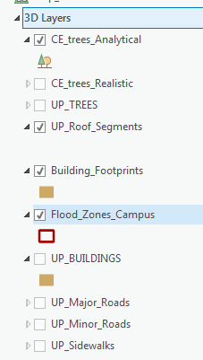
To add it to the 3D scene, in the Contents pane, drag Flood_Zones_Campus from 2D Layers to 3D layers. Placing it below Building_Footprints. Make sure the other 2D layers are off.

Credit: 2016 ArcGIS

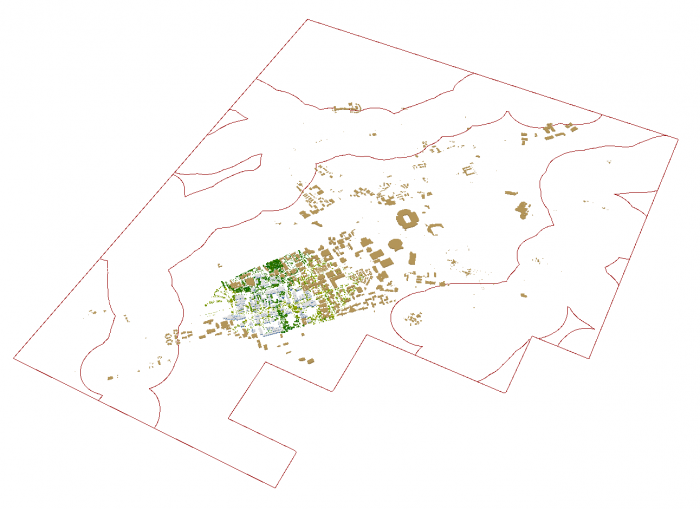Credit: ChoroPhronesis Lab
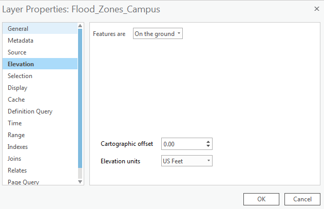
If you cannot see the layer, right-click on the layer and select properties. Click Elevation and make sure the Features are set as "on the ground".

Credit: 2016 ArcGIS
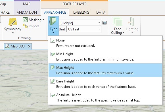
Click Flood_Zones_Campus. On the ribbon, click Appearance. Under Extrusion, choose Max Height as Extrusion Type. Select Height as the field of Extrusion. The Unit will be US Feet.

Credit: 2016 ArcGIS
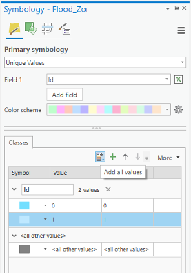
Click Flood_Zones_Campus. On the ribbon, click Appearance and from the Symbology drop-down menu choose Unique Values. In the Symbology pane, the value field is Id. Click Add all values. Change the color of id=0 as Apatite Blue with no border. The color for id=1 will be Sodalite Blue with no border.

Credit: ArcGIS, 2021
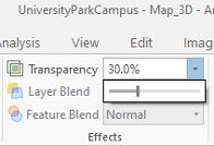
Again select the Flood_Zones_Campus. On the ribbon, click Appearance. On Effects group, change the transparency to 30 percent.

Credit: ArcGIS, 2021
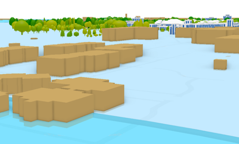
This will be the result:

Credit: ChoroPhronesis Lab
Using your mouse left click and V on the keyboard, navigate through the map. Zoom in to some buildings in different flood zones.

Credit: ChoroPhronesis Lab

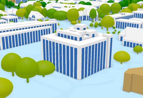Credit: ChoroPhronesis Lab

You can see how less Walker building is flooded compared to peripheral buildings on campus. Changing the height information flood elevation, you can have different results. If you are curious to see how the visualization changes, change the attribute values of Height field in the attribute table.
Make a Screenshot of OldMain in which the level of flooding can be seen. Paste your screenshot into Word and label it Task 1.
Save the Project.