Nexview 3D and Mx™ Software
- Identify the components of the Nexview 3D and their function in measuring light.
- Discuss situations in which misuse of the equipment can result in permanent damage to the instrument.
- Define spatial sampling, numerical aperture, field of view, optical resolution, and how they affect measured surface parameter values.
- Demonstrate proficiency when using the Mx™ software tab.
- Describe the process utilized by the profilometer to obtain measurements and collect the appropriate data.
- Describe the different acquisition options available.
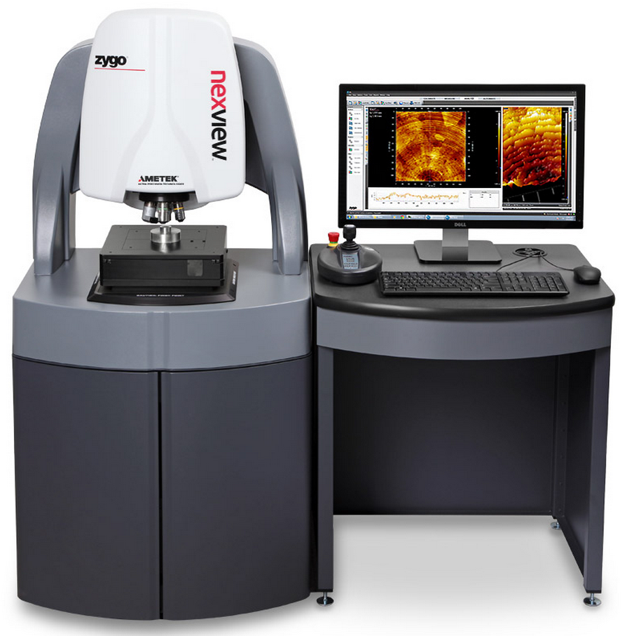
The Nexview 3D Interferometer
Optical Profilers
Optical profilers are interference microscopes, and are used to measure height variations – such as surface roughness – on surfaces, with great precision, using the wavelength of light as the ruler.
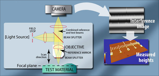
Optical profiling uses the wave properties of light to compare the optical path difference between a test surface and a reference surface. Inside an optical interference profiler, a light beam is split, reflecting half the beam from a test material which is passed through the focal plane of a microscope objective, and the other half of the split beam is reflected from the reference mirror.
Constructive interference occurs when the phase difference between the path lengths is a multiple of 2π, whereas destructive interference occurs when the difference is an odd multiple of π.This creates the light and dark bands known as interference fringes.
Since the reference mirror is of a known flatness, that is, it is as close to perfect flatness as possible, the optical path differences are due to height variances in the test surface.
This interference beam is focused into a digital camera, which sees the constructive interference areas as lighter, and the destructive interference areas as darker.
In the interference image (an "interferogram") below, each transition from light to dark represents one-half a wavelength of difference between the reference path and the test path. If the wavelength is known, it is possible to calculate height differences across a surface, in fractions of a wave. From these height differences, a surface measurement – a 3D surface map, if you will – is obtained.
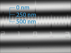
Hypothetically, if the wavelength is 500 nanometers, one could estimate the distance of slope over a full wavelength by looking at the light and dark interference bands – known as interference fringes – in an interferogram. Optical profilers calculate these differences much more accurately than is possible by visual methods.
In practice, an optical profiler scans the material vertically. As the material in the field of view passes through the focal plane, it creates interference. Each level of height in the test material reaches optimal focus (and therefore greatest interference and contrast) at a different time. With well-calibrated optical profilers, accuracy well below a nanometer is possible.
Optical profiling can be used to measure surface finish, roughness, and shape on many surfaces, so long as enough light is reflected back into the objective from the surface.
Much of the content was taken from Zygo's Optical Profiler Basics Webpage
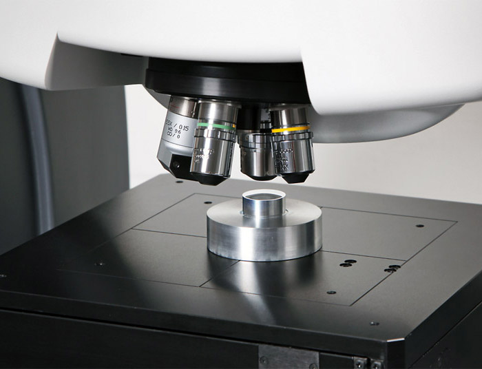
The Instrument and lenses
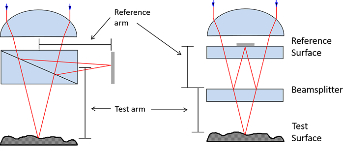
The Nexview interferometer layout
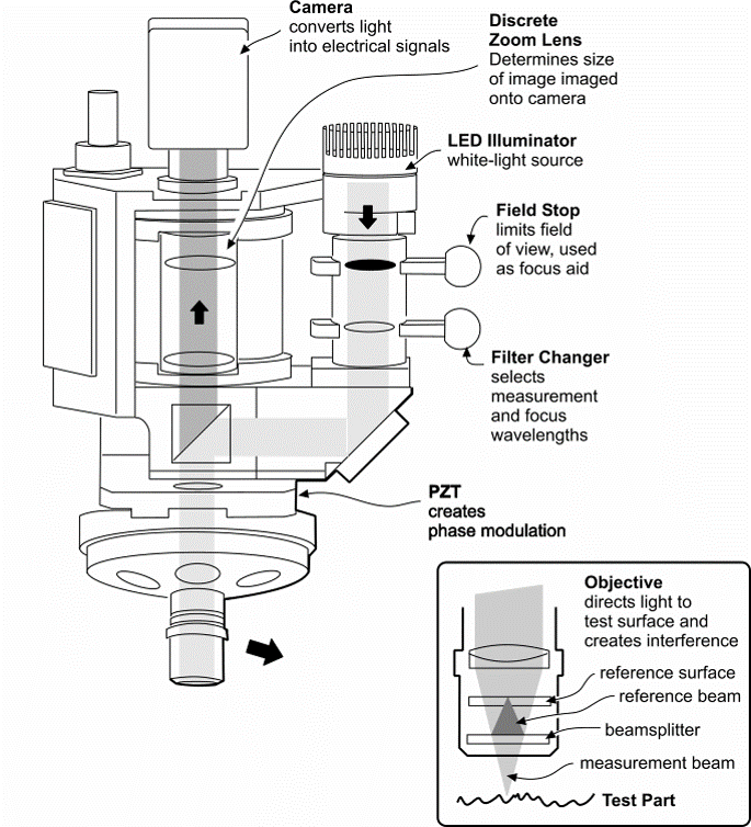
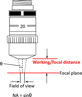
The Zygo surface profilers use interferometers built into the microscope objectives, in either a Michelson (left) or Mirau (right) configuration.
The objectives are calibrated so that the point of zero optical path difference (zero OPD) is the same as the focal distance, i.e., the distance from the beamsplitter to the reference surface is the same as the focal length. This means fringes will appear when the test part is in focus. You will hear working distance, focal distance, and zero OPD used interchangeably during training.
Breaking the Instrument
Optical profilometry is a non-contact imaging technique. The only way to break the instrument is to:
- drive any of the objectives into your sample (odd shaped samples must watch out for all the objectives on the turret!).
- make contact with the objectives on the turret while loading or manipulating your sample. All contact is bad, even the slightest bump or brush.
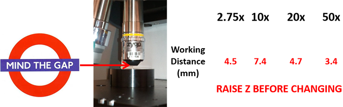
- change objectives without raising Z, allowing clearance for torrent rotation. The objectives on the turret are not parfocal, You must raise Z in order to change lenses.
The Joystick
The joystick controls the manual motion of the stage in X, Y, Z, Pitch, and Roll.
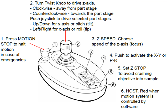
- Fast, Medium, and Slow buttons (3) control the Z-speed (2).
- X-Y or (P)itch-(R)oll control of stage. 200 mm of travel in X and Y and +/- 4 degree of tilt.
- Z-stop setting to avoid crashing objectives into sample.
Spatial Sampling
The detector is a CCD camera with a finite number of pixels. Thus, the optical resolution is also limited by the spatial sampling of the system, i.e., the field of view divided by the number of pixels.
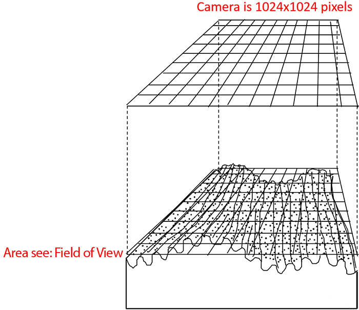
Spatial Sampling = FoV / 1024
Field of View and Numerical Aperture
Field of View
The Field of View (FoV) is the diameter of the circle of light that you see when looking into a microscope. The higher your magnification, the smaller the microscope field of view will be.
The benefits a microscope objective
The imaging system of the Nexview 3D is a microscope objective, which gives the two-fold benefit of:
- higher magnification for small features;
- measurement of rough and sloped surfaces due to higher numerical aperture.
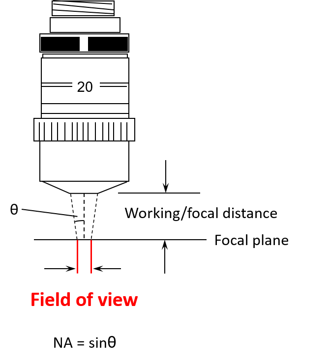
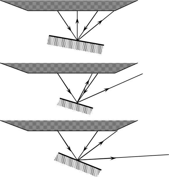
Numerical Aperture (NA)
In optics, the numerical aperture(NA) characterizes the range of angles over which the system can accept or emit light. When the light hits a surface which is highly sloped, it can be reflected to not return up the optical system, and nothing will be detected. This means that higher NA objectives can measure steeper slopes.
Optical Resolution
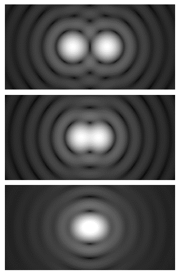
Optical resolution: the Airy disk
Diffraction of light through a circular aperture (like a lens) limits the resolution of any optical system. The best focus of a point source of light from a lens system will form an Airy disk due to this diffraction, rather than the idealized point source.
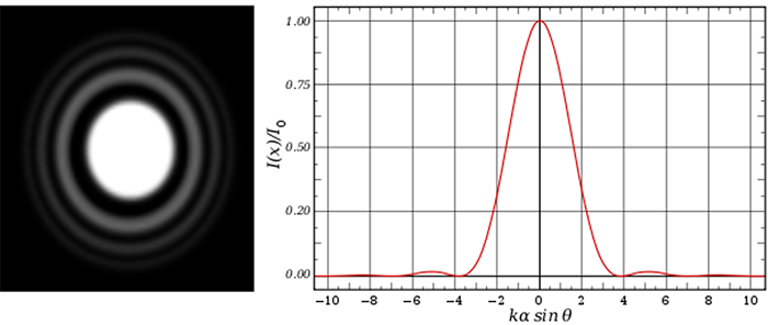
Optical resolution is usually defined as the ability to distinguish two objects which are close together, which is difficult due to the overlap of the Airy disks.
Common criteria for the resolution R:
- The Rayleigh Criterion: R = 0.61λ/NA
- The Sparrow Criterion: R = 0.5λ/NA (used by Zygo)
The effect of diffraction will be a smoothing of features which are too small to resolve sharply.
Note: This resolution is in the lateral (parallel to the focal plane) direction – it is not related to the vertical resolution of the Nexview's measurements.
Optical Resolution of our Objectives
- 2.75x~ 3.563μm
- 10x ~ 950 nm
- 20x ~ 713 nm
- 50x ~ 518 nm
Effects of Optical Resolution and Spatial Sampling on Data
Review:
Optical Resolution = 0.5λ/NA
Spatial Sampling = FOV/1024
Effect of changing optical resolution and spatial sampling
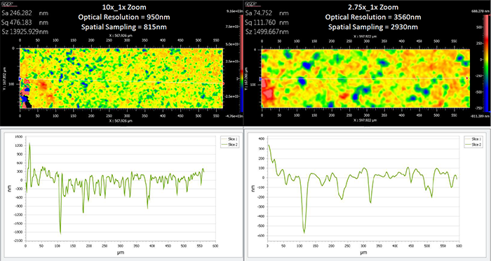
Below is an example of the effect of optical resolution and spatial sampling on information calculated from the surface data. It compares data collected with a 2.75X (NA = 0.08, FOV = 3.00 mm) objective with that from a 10X (NA = 0.3, FOV = 0.83 mm) objective. Since both the NA and the FOV change, our optical resolution and spatial sampling change. The 10X objective is able to capture finer details, and we see the surface roughness increase.
- Sa = surface arithmetic average roughness
- Sq = surface RMS roughness
- Sz = Peak to Valley difference
Effect of changing spatial sampling while using the same optical resolution
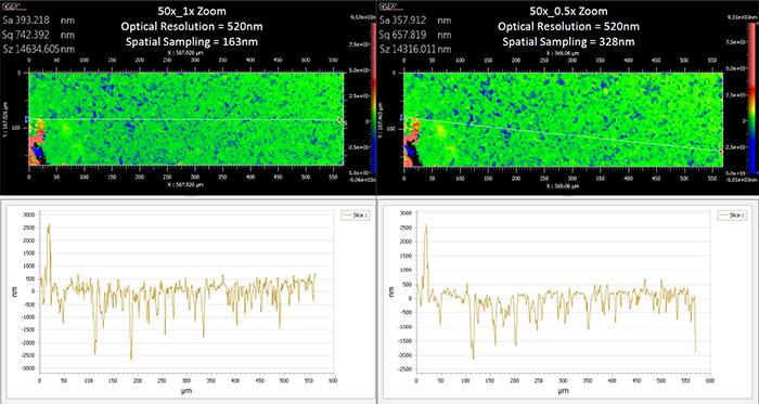
In the below example, the optical resolution is kept the same, both are using the 50X objective (NA = 0.55). However, we are using the internal magnification (0.5X, 1.0X, 2.0X) to change the FOV, which affects the spatial sampling. Even though it has the same resolution, the results collected are affected by the different spatial sampling.
- Sa = surface arithmetic average roughness
- Sq = surface RMS roughness
- Sz = Peak to Valley difference
Note
Be very careful when comparing data from different scans. The above examples illustrate that numerical values from surfaces should only be compared if they were collected using the same optical resolution and spatial sampling.
Working Distance
The working distance (W.D.) is determined by the linear measurement of the objective front lens to the focal plane. In general, the objective working distance decreases as the magnification and numerical aperture both increase.
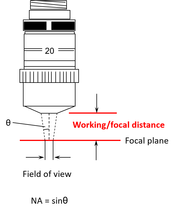
The working distance is the distance from the front of the lens to the focal plane. The objectives are designed that this is also where zero OPD occurs. Because of this, the terms W.D., focus, and zero OPD are often used interchangeably.
Z-Stop
The Z-Stop protects the optical profilometer in the Z direction. It needs to be set for each sample, with care taken to set a proper distance.
Set Z-Stop (CRITICAL)
- Verify the working distance of the objective. (See table below.)
- Check Z-Stop status (what color is Z-stop light on joystick?).
- Red = At Z-stop position.
- Green = Above Z-stop position.
- Flashing Red = No Z-stop is set. USE EXTREME CAUTION (instrument will beep as you move in Z).
- Only pay attention to the space between the objective and the top of your sample. No need to look at the PC, your cell phone, your friend next to you. Just focus on the objective-sample gap.
- The ideal Z-stop position is defined as a distance between objective and sample surface that is less than the working distance and allows for the scan to reach just below the lowest region of the surface. Too low a Z-stop can put the instrument at risk; a Z-stop too close to the Working Distance could lead to software errors when you try to scan.
- Use Fast only at distances greater than 20mm from the sample. Press Z-stop button so the light is flashing RED and begin a downward focus until you arrive at approximately 20mm. Push Medium and continue towards the surface until an appropriate Z-stop position. Never use “FAST” speed when nearing sample surface (<20mm)
- Press Z-stop so the light is now solid RED.
- Use focus aid and raise Z to focus.
What is a good Z-Stop position?
The simple answer here is one that allows the instrument to scan low enough to scan through all parts of your surface AND prevents the instrument from being driven into your sample. Below are illustrated examples of an improper and proper Z-stops.
Most important thing to remember when setting the Z-Stop is to remember you do this manually by watching the objective and your sample directly. It is never to be set watching the computer screen with the software.
Nexview Objective Selection Guide
Objectives highlighted in yellow are the ones currently installed on the Nexview 3D turret.
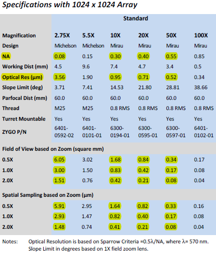
The Nexview 3D has 4 objectives on the turret and 3 internal magnifications, giving 12 FOV (highlighted in the middle of the above image), some of which overlap.
So, which do you choose?
Most often it is the size of what you are trying to measure which determines the FOV you want to work at.
But what about the overlapping fields of view; which objective should I use?
In the case of overlapping FOV; for example, the 10X objective can be used as a 5X, 10X, or 20X, and the 20X objective can be used as a 10X, 20X, or 40X. They both have 10X and 20X options; so, which do I choose? The 20X is the choice over the 10X on flatter samples as it has the better NA, which means you have better optical resolution. However, the 10X has a much further working distance and can be useful on rougher samples when we can't use the 20X.
These are the things you consider when making your objective choice.
Pitch, roll, and null
The lateral/Y axis, or pitch axis is an imaginary line running horizontally across the sample through the center of gravity. A pitch motion is an up-or-down movement of the front or back of your sample as mounted on the stage.
The longitudinal/X axis, or roll axis is an imaginary line running horizontally though the length of the sample through its center of gravity. A roll motion is a side-to-side movement or tilting left or right of your sample as mounted on the stage.
To "null" the fringes is to adjust the pitch and roll of your sample so it is parallel to the plan of the interference fringes, which is perpendicular to the Z-scan axis.
Nulling the fringes predominantly helps you with minimizing the scan length needed to measure your surface.
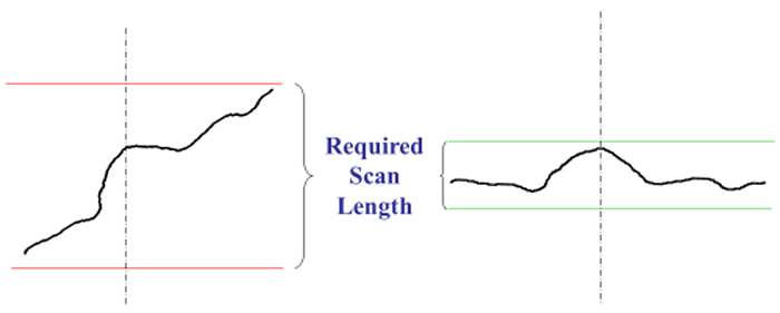
An example for Smooth Flat Surfaces
To "null" the fringes is to adjust the pitch and roll of your sample so it is parallel to the plan of the interference fringes, which is perpendicular to the Z-scan axis.
The cartoons to the right show the impact on scan length when a flat part is nulled properly (cartoon on the right with the small green scan length outlined is nulled properly). If the differences in scan length on in a few μm to tens of μm it likely doesn't matter much. If the differences are in the 100s of μm, it will greatly affect your collection time and care should be taken to null the surface as best you can.
For a Smooth Flat Part, adjust for high contrast and the least number of fringes. On very flat parts, it is possible to null the surface such that the fringes take up the entire field of view
Below is a video showing the actual field of view (right) and a cartoon (left) depicting what is happening on a tilted smooth flat part as the instrument is moved up in Z with the joystick. Notice how the fringes travel across the field of view from upper right to lower left. The fringes indicate that not only is the sample tilted, the direction of travel describes how it's tilted. The fringe travel indicates, in this example, that the front left corner of the stage is higher.
Nulling the stage for a smooth flat part gets the sample surface and the Z-travel perpendicular, which means the surface is parallel to the fringes now. As the instrument is moved up in Z now, the fringes can be seen individually as they flash by.
An example for Textured Surfaces
To "null" the fringes is to adjust the pitch and roll of your sample so it is parallel to the plan of the interference fringes, which is perpendicular to the Z-scan axis.
Textured surfaces are very similar to flat surfaces, though it can be harder to see the trend in the tilt of the sample. The goal is to null the overall sample tilt to minimize the scan length.
On Textured or Rough Flat Part the fringes are in smaller isolated areas. Center the fringes and adjust the focus between the high and low fringes. The distinct lines that were seen for smooth surface are broken up with the varying topography of a rough or textured surface. Nulling the fringes involves adjusting the fringes so they enter and leave the field of view without any discernible trend in X or Y tilt.
Below is a video showing the actual field of view (right) and a cartoon (left) depicting what is happening on a tilted textured or rough part as the instrument is moved up in Z with the joystick. Notice how the fringes travel across the field of view from lower right to upper left. The fringes indicate that not only is the sample tilted, the direction of travel describes how it's tilted. The fringe travel indicates, in this example, that the back left corner of the stage is higher.
Nulling the stage for a textured or rough part also gets the sample surface and the Z-travel perpendicular, which means the surface is parallel to the fringes now. As the instrument is moved up in Z now,fringes enter and leave the field of view without any discernible trend in X or Y tilt.
An example for Curved Surfaces
To "null" the fringes is to adjust the pitch and roll of your sample so it is parallel to the plan of the interference fringes, which is perpendicular to the Z-scan axis.
On a Spherical Part, adjust the stage and the focus to center the circular fringe pattern. This can be done by moving in X/Y or in P/R, depending on what you are trying to measure. Depending on the curvature of the sample, nulling a spherical sample can significantly reduce collection time.
Below is a video showing the actual field of view (right) and a cartoon (let) depicting what is happening on a curved part as the instrument is moved up in Z with the joystick. Notice how the fringes travel across the field of view from right to left. The fringes indicate that not only is the sample offset, the direction of travel describes how it's offset. The fringe travel indicates, in this example, that the back sample curvature continues to rise to the left. Either X/Y or P/R can be adjusted to center the circular pattern depending on the users specific needs.
Nulling the stage for a curved part minimizes the total sample height within the field of view. As the instrument is moved up in Z now, the fringes go through a circular, bullseye pattern centered in the field of view.
Relationship between working distance, Z-stop, and scan length
Review of some important concepts
The working distance is the distance from the front of the lens housing down to the focal plane of the objective. We commonly use working distance, focal plane, and zero optical path difference interchangeably. The focal plane of the objective must scan all the way through the sample surface (from above, down through, and then below the highest and lowest parts of the surface in the FoV of the scan or stitch).
Z-Stop
The Z-Stop is a hard stop for both the user and the software, set before working in the software, to allow the focal plane to scan through the required scan length but prevent any part of the instrument from making contact with any part of the sample or sample mounts that may be in use.
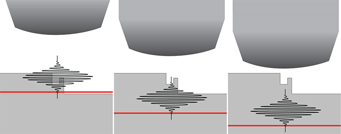
In the above image, we have three different Z-stop (denoted by the red line) settings. On the left, the Z-stop is set too close to the surface, and you will not get any good data. In the middle, the lower Z-stop allows you to collect some information from the higher parts of the sample surface, but it does not take into account the proper distance the width of the fringes must travel through to reach the lowest part of the sample. The image on the left shows a Z-stop that not only allows the instrument to scan the width of the fringes through all of the surface topography, but also protects the objective from being driven into the sample by the user or the software.
Scan Length
Scan length is discussed in the section on MX™ measure tab, but we will take this into consideration here for a moment to get you thinking about things to come.
Once you have a proper Z-stop set. Setting up the proper scan requires the user to set up a proper scan start position and scan length so the width of the fringes can be scanned entirely through the surface topography. An illustration of what the system looks like scanning is depicted below. Notice how the instrument moves with respect to start and end scan. This will be covered in more detail in the next sections.
The Mx™ Measure tab
The Measure tab is where all data collection originates.
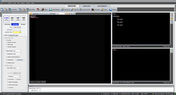
Top Control Bar

The Top Control Bar - Details

Load application, Load application settings, Load Data - only Load Data is useful to users.

Save application, Save application settings, Save Data - only Save Data is useful to users.

Home - term given to the default screen for a particular instrument and application.
Masks - opens the mask editor.
Auto Sequence - opens the auto sequence editor.
Auto Focus - the instrument scans through a set Z range and attempts to locate the fringes.

Auto Tilt - the instrument scans through a set Z range and attempts to remove the sample tilt.
Auto Focus and Tilt - the instrument performs an auto focus followed by an auto tilt.

Focus Aid (F8) - opens the focus aid.

Auto LL (F9) - adjust the camera shutter and light level. Should be done with the center fringe in the video display.

Measure (F12) - take a measurement.
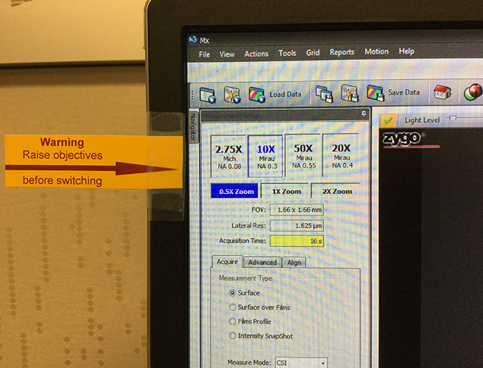
Objective Selection
The objectives selector
There are 4 objectives and 3 internal magnifications giving us 12 different combinations of FOV and Optical Resolution.
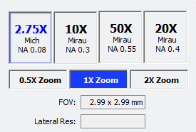
Changing the objective requires the user to raise the instrument up before selecting the new objective (which rotates the turret).
Failing to do so could cause significant damage to the lenses and scanner.
There is a warning reminder on the side of the monitor.
Measurement Type
Selects what characteristics of the test part are to be measured.
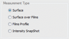
Surface - Use this mode when measuring surface topography on opaque parts.
Surface Over Film - Use this mode when measuring the top surface topography on a part with transparent films. This mode does not provide any information about the underlying film(s). Adds Films tab.
Films Profile - Use this mode when measuring the top surface topography and/or either the bottom surface topography or the film thickness. This mode only returns information about the top-most film when measuring parts with multi-layer film stacks. Adds Films tab.
Intensity SnapShot - Use this mode to measure a 2D intensity snapshot of the scene as represented in the Live Display. The mode may be useful for lateral metrology or feature alignment, but will not provide any information about the surface topography.
Measure Mode and Z Resolution
Measure Mode
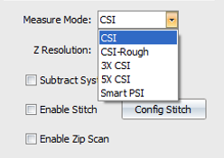
CSI - Coherence Scanning Interferometry -This is the default starting point and good for most parts.
CSI - Rough - This mode makes CSI measurements using a narrower bandwidth illumination spectrum to improve performance on rough parts and sometimes on parts with high slopes. It generally improves data coverage, but with a decrease in vertical resolution. The improvement is part-dependent and should be compared with CSI results.
3X CSI - This mode makes sub-Nyquist CSI measurements at 3X the nominal scan rate to provide higher throughput, but with a decrease in vertical resolution. 3X CSI measurements are compatible with PZT and extended scans.
5X CSI - This mode makes sub-Nyquist CSI measurements at 5X the nominal scan rate to provide even higher throughput, but with a further decrease in vertical resolution.
Smart PSI - Smart PSI combines a CSI scan to focus the instrument and determine the coherence profile of the surface with a series of rapid PSI (phase-shifting interferometry) measurements to determine the high-resolution phase profile of the surface. This mode is ideal for smooth parts with low departure (PV < few microns) and is the best option for super-smooth parts.
Z Resolution
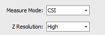
High - The phase and coherence profiles are combined to provide the final height map. Provides highest vertical resolution.
Normal - The coherence profile is taken to be the surface height. Provides most data on challenging parts, but at lower vertical resolution.
Subtract System Reference, Enable Stitch, and Enable Zip Scan options

Subtract System Reference - Select check box to use a system reference file. This is used to improve instrument performance by minimizing noise. There must be a valid 3D reference calibration for this to function.
Enable Stitch - Select check box to measure using a configured stitch routine. Stitching is used to analyze areas larger than a single measurement; multiple measurements are combined together.
Enable Zip Scan - Select check box to activate a Zip Scan sequence. A Zip Scan is two or more groups of measurements separated by a vertical distance. A Zip Scan is useful for parts with isolated heights; it effectively extends the scanner range.
Acquisition Options
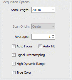
Acquisition Options controls things such as the scan length, scan origin (depending on which motor you are scanning on), averaging, signal over sampling HDR, and true color. The most common reason for dropped pixels in an image is incorrect scan length and/or scan origin. The following sections cover more detail.
7.1: Scan Length and Scan Origin
Scan Length - Selects the vertical scan length. The longer the scan, the greater the height measuring capability, and the longer the measurement time. It is recommended to set to the smallest value that encompasses the part details. When set to Extended, the user enters the length of the scan, which is longer than the selectable lengths. The value entered should be the vertical range of detail in the part plus 10%.
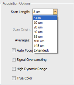
Scan Lengths have two options: It is very important to understand the difference between the two scan length options.
- Numerical scan length choices from 5um-145um (length options change depending on measure type and measure mode) are bi-polar scans which utilize the PZT scanner with only a center scan origin option.
- Extended scans use the Z-motor and you have options for setting the scan origin to top, center, or bottom.
Scan Origin - Selects the location of the part relative to the full scan range when the scan is initiated. Scan profiles for each control option are shown below.
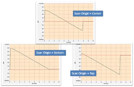
Important to note that the scanner only collects data on the downward part of the motion.
7.2: Averages, Auto Focus, and Auto Tilt
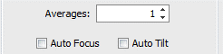
Averages - Specifies the number of measurements to average together to reduce random measurement noise. Averaging increases measurement time.
Auto Focus - Select the check box to perform auto focus before each measurement. The Auto Focus function is useful when the surface of the part being measured does not fall within the current scan range of the sensor. Auto focus will automatically scan at faster rate (depending on the controls) over a longer distance in Z (depending on the controls) to find the surface of the part, then move the sensor head so that the part surface is nominally centered in the middle of the sensor's scan range.
Auto Tilt - Select the check box to perform auto tilt before each measurement.
7.3: Signal oversampling, High Dynamic Range, and True Color
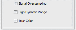
Signal Oversampling - expense of longer measurement time. Signal Oversampling is used to extract very weak signals from challenging surfaces such as those with large roughness or steep slopes. Signal Oversampling can be used in conjunction with CSI or Films measure modes and can be combined with other acquisition options such as Zip Scan, HDR, and True Color. When using oversampling and extended scan, be sure that the SureScan control is set to Off.
High Dynamic Range - Select the check box accommodate parts with a wide variation in reflectivity. This option causes the system to take sequential measurements at up to 3 discrete light levels to accommodate wide variations in part reflectivity. The two measurements are combined to maximize the amount of data and quality of the surface data produced. When the High Dynamic Range mode is checked, an HDR tab is added to the Measurement Setup panel for setting the various light levels.
True Color - Select the check box to enable the collection of a full color surface image for all data points in the topography map.
- Immediately following the metrology scan, a secondary acquisition is automatically executed to collect true color information about the surface at the point of best focus for each data point in the camera.
- Provides full color surface image for all data points in the topography map.
- To display color information in the 2D and 3D surface maps, select the True Color icon in the plot toolbar or context menu.
- Color information is stored with the .datx data file format.
Configure Stitch
The Configure Stitch Section
Stitching makes several measurements of the test part as it is moved by the motorized stage and then combines or stitches the multiple data sets into one. Effectively, it increases the field of view without compromising lateral or vertical resolution. The final graphics and results are based on the entire measured area.
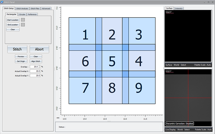
8.1: The Stitch Setup Tab
This section of the stitch panel allows the user to set up a stitch based on what they see in the live display.
The users sets the origin position (position 1). The user then sets the start and end locations. This allows the software to determine how many rows and columns are required to stitch the chosen area based on the current field of view (objective and internal magnification).
It also contains the Stitch button, controls for the size of the overlap region, and the ability to preview the area that will be scanned.
8.2: The Stitch Analysis Tab
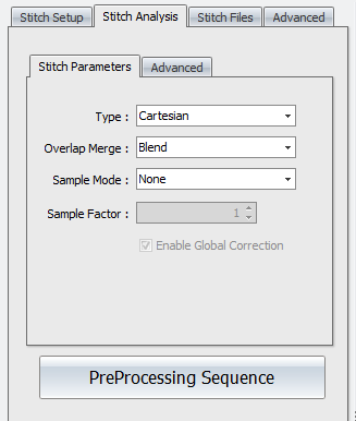
Stitch Analysis controls are used to specify how sites are aligned and how overlap areas are processed.
Stitch Analysis- Stitch Parameters
Type - Selects how sites are aligned. Options are Adjust XY, Cartesian, or Overlay. Adjust XY matches and aligns sites in x and y axes. Cartesian matches and aligns sites in x, y, z, pitch, and roll (5 axes). Overlay aligns sites based on stage coordinates.
Overlap Merge - Selects what happens in overlap regions. Options are Blend, Average, or No Merge. Blend does an interpolation (fitting) of the sites. Average averages the data in the overlap regions. No Merge does not merge overlapping areas.
Sample Mode - Selects how sites are sub sampled. This is typically used to increase throughput when stitch sequences are large (more than 100 sites). Options are None, Bin, or Skip. None means no sub sampling is performed. Bin uses a convolution of camera data and then downscales and averages data. Skip reduces the number of data points by using row and column data as determined by the Sample Factor control.
Sample Factor - Determines the functionality of the Sample Mode control. When Sample Mode is Bin, it is how many pixels get binned together. When Sample Mode is Skip, it determines the number of rows and columns of pixels to skip (or not use).
Enable Global Correction - When this check box is selected, a Cartesian algorithm is also applied after adjusting X,Y position using the Adjust XY algorithm. Only available when Type is Adjust XY.
Preprocessing Sequence - Opens a processing sequence window. This is used to specify data processing operations on the raw stitch data before it is all stitched together. See Data Processing for details on using this feature. For example, if the combined stitch area results in multiple tilted planes with nothing connecting between sites, use the remove form function in the Sequence tool.
Stitch Analysis- Advanced
Search Window - Specifies how much searching is attempted when aligning sites to each other. Too large of a search area increases processing time. Too small of an area may provide insufficient matching. The Automatic setting is determined internally and displayed. To override the Automatic setting, select the Manual radio button and enter a dimension.
Lateral Resolution - This attribute shows the lateral resolution of the current instrument configuration.
Search Window - This attribute shows the size of the search window in pixels.
8.3: The Stitch Files Tab
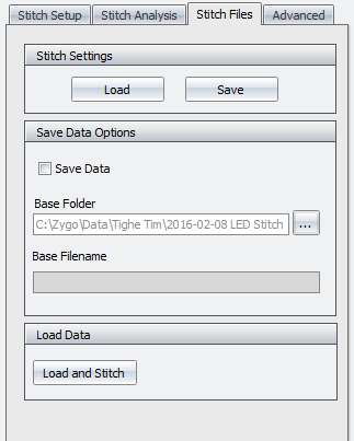
The Stitch Files tab allows the user to save the individual files of a stitch in case there is a problem during stitch. Scans which have had a problem will show up as red when completed (successful scans show up as green). If the user has saved the individual files, they can go back and just recollect the areas which had issues and then restitch the image with the software.
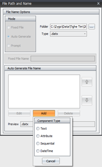
To use this feature, the user must check the Save Data option. Then click the ... button to the right of the base folder option. This will open up another dialog which allows the user to direct the software to the proper folder, add text for a filename, add sequential so you can keep track of which individual file is which, etc.
8.4: The Stitch Advanced Tab
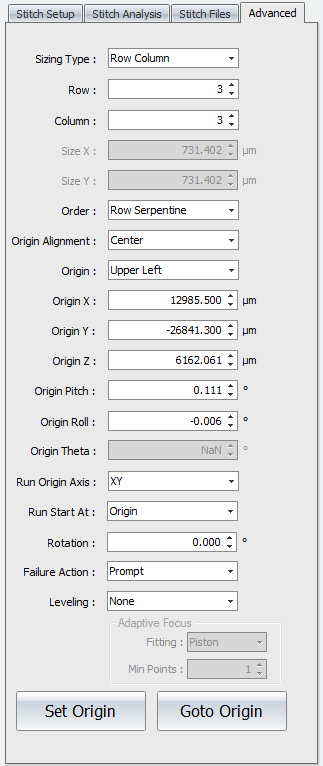
Stitch Panel Advanced Tab
Controls accessed under the Advanced tab are used to fine-tune stitch sequences.
Sizing Type - Selects how the size of the stitched area is defined. Options are Size or Row Column. Size requires lateral dimension entries in the Size X and Size Y controls. Row Column requires an entry in the corresponding Row and Column controls.
Row - Specifies the number of horizontal rows in the stitch sequence.
Column - Specifies the number of vertical columns in the stitch sequence.
Size X - Specifies the size of the overall stitched image in the x-axis.
Size Y - Specifies the size of the overall stitched image in the y-axis.
Order - Selects how to traverse the part rows and columns, in a serpentine or raster fashion. Options are Row Raster, Row Serpentine, Column Raster, or Column Serpentine. Raster order measures sites in one direction. At the end of a row or column, the stitch continues after traversing back to the beginning of the row or column. Serpentine order winds back and forth measuring sites as it goes.
Origin Alignment - Selects the site located at the origin; the field of view is aligned such that the origin stage position is either the Center or Corner.
Origin - Selects the corner where the stitch sequence begins. Options are Upper Left, Upper Right, Lower Left, or Lower Right.
Origin X - Specifies or displays the origin of the stitched image in the x-axis.
Origin Y - Specifies or displays the origin of the stitched image in the y-axis.
Origin Z - Specifies or displays the origin of the stitched image in the z-axis.
Origin Pitch - Specifies or displays the origin of the stitched image in the pitch axis.
Origin Roll - Specifies or displays the origin of the stitched image in the roll axis.
Origin Theta - Specifies or displays the origin of the stitched image in the theta axis (not applicable with PSU hardware).
Run Origin Axis - Determines the axes to move when the stitch or pattern runs and goes to the origin position. Options are XY (default) or All. XY moves only in x and y at the first site. All moves in x, y, z, pitch, and roll at the first site; all others sites only move in x, y, and z.
Run Start At - Determines where the stitch sequence or pattern is started. Options are Origin or Current Position. Origin goes to the origin and runs the stitch or pattern. Current Position sets the origin at the current site location and runs the stitch or pattern, effectively shifting the locations.
Rotation - Rotates the stitch grid. This useful when the part is skewed in reference to the instrument axes.
Failure Action - Selects the action to take if there is a measurement error during a stitch sequence. Options are Continue, Prompt, Retry, Retry After Completion. Continue ignores the error and goes to the next site. Prompt asks the user what they would like to do when a failure is encountered. Retry tries to measure the site again. Retry After Completion goes back to the sites with errors and tries again.
Leveling - Selects how to adjust in the z axis during the stitch sequence or pattern to compensate for general form in the part being measured. Options are None (default), Linear Manual Adjust, Linear Store, Tilt, Cylinder, or Adaptive Focus.
Training Completion
If you have not done so already, please submit a request for training through the MCL homepage to set up a time to complete the in person training.