Lesson 6: Surface Patterns of Pressure and Wind
Motivate...
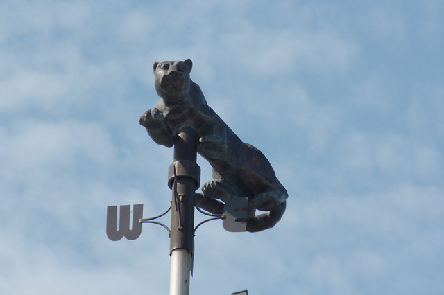
In his 1965 song, "Subterranean Homesick Blues [4]," Bob Dylan famously quipped, "you don't need a weatherman to know which way the wind blows." I'm sure he didn't know at the time that this lyric would become one of the most influential in modern music history (it's apparently a favorite among judges and lawyers [5] in legal proceedings). When it comes to weather forecasting, Bob is right -- kind of. You don't need a weather forecaster to know which way the wind blows right now. Just about anyone can take their own observation, or look at a weather vane (see photograph at the right) if one happens to be nearby. But, you do need a competent weather forecaster to consistently tell you which way the wind will blow in the future.
Although wind may not get much attention in casual discussions of the weather (you don't often hear people say, "I wonder if it's going to be windy this weekend."), wind forecasting is really important. For starters, if you think back to our lesson on controllers of temperature, several of them were based on the wind (such as temperature advection and mechanical mixing of eddies caused by the wind). So, if weather forecasters make significant errors in their wind forecasts, the accuracy of temperature forecasts can suffer, too.
Furthermore, wind forecasting is pivotal in many other contexts. Sailors and pilots, for example, rely on accurate wind forecasts for safe and successful travel. The wind is also increasingly being used as an energy source via the generation of electricity from wind farms [6]. These are just a few examples, but in a nutshell, being able to predict wind direction and speed accurately is beneficial in many settings. Indeed, we do need weather forecasters to know which way the wind will blow.
In this lesson, we're going to talk about the main forces that cause the wind to blow as it does. You'll learn that the main driving force of the wind is caused by pressure differences across the earth's surface, but other forces, namely the "Coriolis Force" and friction, also impact wind speed and direction. With an understanding of these forces, you'll be able to learn about how air circulates around high- and low-pressure systems, and how pressure and winds change across air-mass boundaries (fronts). Ultimately, this lesson won't make you a wind forecasting expert, but by the end, you should be able to interpret basic surface maps like this one [7], and use the pattern of isobars to determine whether winds will be relatively fast or slow, as well as determine what direction winds will blow from.
So, this lesson has lots of useful weather analysis skills, and our first stop is to take a closer look at pressure. As you're about to see, this is a "weighty" topic! Let's get started!
Under Pressure
Prioritize...
When you've finished this page, you should be able relate surface pressure to the weight of an air column above a point. You should also be able to express pressure with the proper units and discuss the typical range of sea-level pressure on Earth.
Read...
"Pressure...pushing down on me, pressing down on you..."
Those lyrics come from this section's theme song -- ”Under Pressure“ by Queen (featuring David Bowie) [8] from 1981. As we start our investigations of pressure (and ultimately wind), we have to start with the basics. For starters, what is pressure? On that matter, Queen basically nailed it. It's a force that pushes down on me and you (and everything else). More formally, you may remember from a high school science class that pressure is defined as a force per unit area.
Meteorologists are concerned about atmospheric pressure -- the pressure exerted by air molecules. The pressure exerted by air molecules at a weather station is approximately the weight of the air in a column that extends from a fixed area on the ground to the top of the atmosphere. At sea level, the weight of a column of air on one square inch of area is roughly 14.7 pounds, resulting in an air pressure of 14.7 pounds per square inch. For perspective, that amounts to a total force of more than 2 tons on just the area covered by a single base on a baseball field (an 18-inch by 18-inch area). Surprised?
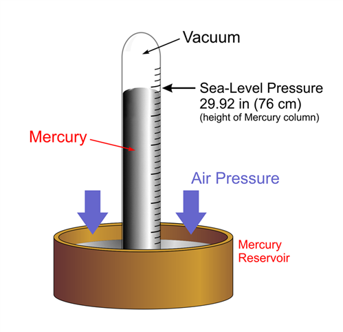
Meteorologists typically don't work with pressure in pounds per square inch, however. Most home barometers (instruments for measuring atmospheric pressure), for example, express pressure in inches of mercury, which is based on the mercury barometer [9]. Mercury barometers measured pressure after air was evacuated from a glass tube, and the open end of the tube was immersed in a reservoir of mercury, allowing air pressure to force mercury to rise in the glass tube. At sea level, the standard height of the mercury column is 29.92 inches. More commonly, meteorologists often work with pressure in units of millibars (abbreviated "mb"). For reference, an atmospheric pressure of 14.7 pounds per square inch (when the height of a Mercury barometer would be 29.92 inches) is equal to about 1013 millibars.
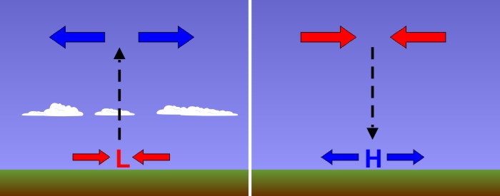
The connection between surface pressure and the weight of a column of air that extends above the surface has many important consequences. For starters, processes that reduce the weight of an air column also act to decrease the surface pressure. On the other hand, processes that add weight to air columns act to increase surface pressure. Evolving horizontal patterns of air pressure are crucial to weather forecasting, which is one of the reasons why forecasters pay such close attention to centers of highest and lowest pressure on weather maps (typically marked by a blue "H" and a red "L", respectively). In a very general sense, low-pressure systems tend to bring inclement weather (clouds and precipitation), while high pressure systems tend to bring "fair" weather (sunshine and relatively calm conditions).
The bottom line here is that when you hear meteorologists refer to a "low pressure system," what they are really talking about is a "lightweight." In other words, the air column above the center of a low weighs less than any of the surrounding air columns. On the flip side, a high pressure system is a "heavyweight" because the air column above the center of the high weighs more than any of the surrounding air columns. Now, I should point out that the difference in pressure between a run-of-the mill high-pressure system and a pretty strong low-pressure system is only about five percent. In the image on the right, for example, the difference between the labeled high and low is only 32 millibars (1018 millibars - 986 millibars), so the difference was even less than five percent in this case. Still, these differences have very important consequences for the weather, as you'll learn!
To get a feel for the range of pressures at sea-level, check out the graph below. Remember that standard sea-level pressure is around 1013 millibars, while a very strong high pressure system in the winter may measure around 1050 millibars. On the other hand, a representative value for sea-level pressure at the center of a formidable low-pressure system that can cause, for example, heavy snow during winter might be in the neighborhood of 960 to 980 mb.
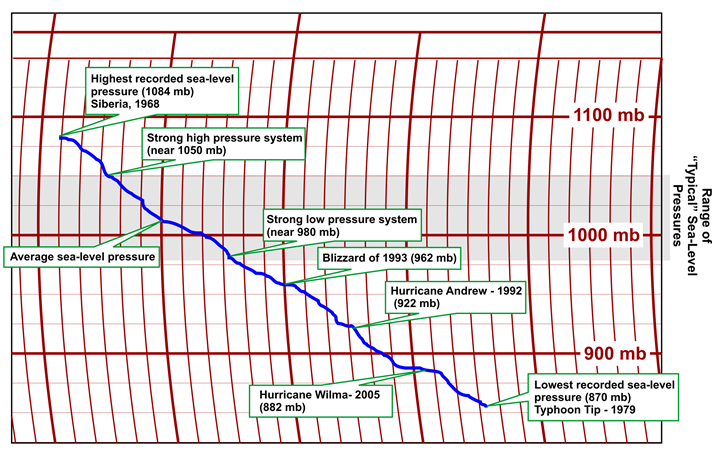
The bottom of the observed range of sea-level pressures is populated by the "kings" of all low-pressure systems on our planet -- hurricanes (called "typhoons" in some parts of the world). Very intense hurricanes can have sea-level pressures down near 900 millibars. In 2017, for example, at its peak intensity, Hurricane Maria [10] had a minimum sea-level pressure of 908 millibars. The storm later went on to devastate Puerto Rico, and its fierce winds completely destroyed the island's NEXRAD Doppler radar (this short video highlights Maria's damage to Puerto Rico [11], and includes some stunning images of the damage to the radar, if you're interested). A handful of hurricanes and typhoons globally have even had sea-level pressures drop a bit below 900 millibars.
Ultimately, the pressures associated with very intense hurricanes and very strong high-pressure systems in the winter (more than 1050 millibars) are pretty rare. As a general guideline, nearly all sea-level pressures lie between 950 millibars and 1050 millibars, with most sea-level pressure readings falling between 980 millibars and 1040 millibars.
You'll want to keep this range in mind, because it will come in handy as we interpret pressure data from various maps. You also may have noticed that I was careful to specify "sea-level" pressure when discussing pressure values. Why is that? You'll find out in the next section as we explore contour maps of pressure (maps of "isobars"). Read on.
Decoding Pressure
Prioritize...
At the end of this section, you should be able to discuss the change of atmospheric pressure with increasing height, the difference between "station pressure" and "sea-level pressure," analyze maps of isobars (contoured maps of pressure), and decode pressure from a station model.
Read...
In the last section, our discussion of pressure was focused on the pressure at sea level. But, most of the United States (and the rest of the world's land masses) aren't at sea level, so why make that distinction? Well, in order to analyze the horizontal patterns of surface air pressure that govern weather, meteorologists require a "level playing field," and that's why they're interested in "sea-level pressure."
To see what I mean, consider this: if you brought a barometer with you on a trip to Denver, Colorado (elevation about one mile above sea level), it would regularly measure a pressure of about 850 millibars. That's much lower than the typical range of sea-level pressures we talked about in the previous section. The pressure on your barometer would be so low because pressure decreases with increasing height everywhere in the atmosphere. The reason why that's the case is fairly intuitive: the higher the altitude, the less air (and weight) there is above you in an atmospheric column. In fact, pressure at the top of the troposphere [12] is typically less than 300 millibars (less than 30 percent of the pressure at sea level).
So, the fact that pressure decreases with increasing height explains why the surface pressure at high elevation locations (like Denver) is much lower than at sea level. For meteorologists, surface pressure's dependence on elevation presents a bit of a problem. To see what I mean, check out the map of long-term average surface pressure (called station pressure) across the United States below.
The first thing you might notice on the map is the area of very low pressures in the Rocky Mountains (less than 780 millibars in some areas). Is there some kind of monster low-pressure system permanently parked in the Rockies? Of course not! The station pressures are always low there because of the high elevations in the Rockies. The dramatic variation in station pressure based on elevation makes it virtually impossible for meteorologists to use station pressure to track centers of high and low pressure. Regardless of the strength and position of various high- and low-pressure systems, the map of station pressure would always look something like the one above (lowest pressures in the highest-elevation regions). So, in order to level the playing field, meteorologists adjust station pressure to sea level.
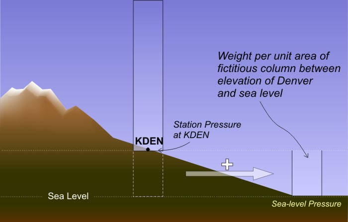
By adjusting to sea level, meteorologists are essentially pretending that high-elevation locations (like Denver) are located at sea level, and as such, they adjust all barometer readings to what they would be if they were located at sea level. To do so, meteorologists "correct" the station pressure to sea level by estimating the weight of an imaginary column of air that extends from station to sea level. I'm skipping the details, but the bottom line is that this estimated weight of the imaginary air column gets converted into a pressure adjustment that is added to the observed station pressure (this schematic may help you visualize the adjustment process [13]). While the estimating process isn't perfect (especially for very high elevation locations), the end result is a sea-level pressure value that can be used to plot useful weather maps, which help meteorologists track high- and low-pressure systems more effectively.
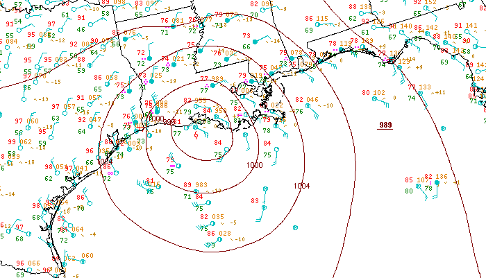
Thus, the contour maps of pressure that meteorologists most commonly work with (and that we'll most commonly work with) are maps of sea-level isobars (remember that "isobar" is the name of a contour of equal pressure). Maps of sea-level isobars help weather forecasters quickly spot areas of low and high pressure, which can help them identify areas of potentially stormy weather. For example, check out the analysis of sea-level pressure from 12Z on October 30, 2017 below, and note the strong low-pressure system centered just north of New York state (marked by the "L") in the Canadian Province of Quebec).
If you remember how to interpret contour maps, you should be able to estimate the pressure at the center of this strong low. The contour interval on this map is four millibars and the innermost labeled closed isobar around the low is 984 millibars. There's one unlabeled closed isobar inside the 984-millibar isobar, which represents 980 millibars. The center of the low is located inside that isobar, so its lowest pressure must have been less than 980 millibars, but greater than 976 millibars (otherwise there would have been a 976-millibar isobar drawn).
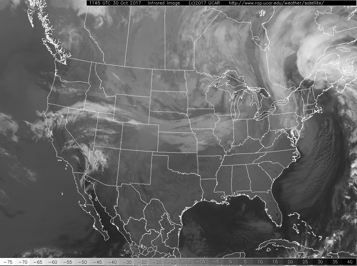
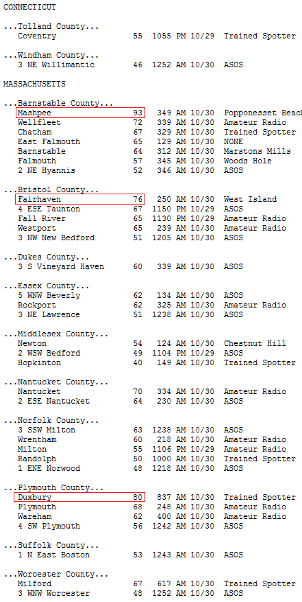
To place this sea-level pressure in perspective, check out the barograph showing the range of sea-level pressures [14] again. A sea-level pressure less than 980 millibars represents a pretty strong low, so we might expect some pretty "active" (stormy) weather in the Northeast U.S. around the low-pressure system depicted above. Indeed, that was the case! Check out the 1145Z infrared satellite image from October 30 [15], and note the fairly bright white shading in the region, indicative of an organized area of cold cloud tops. This storm brought drenching rains to the Northeast, along with damaging wind gusts (the National Weather Service office in Boston compiled this list of strongest wind gusts [16], including several reports of gusts greater than 75 miles per hour). More than a million people lost power in New England from this storm.
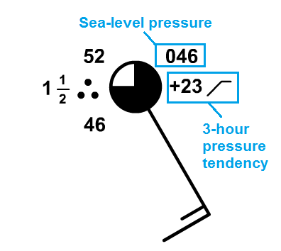
So, where do the pressure observations come from that are used to make maps of sea-level isobars like the one above? Station pressure is routinely measured at surface weather stations (along with temperature, dew point, wind, etc.) and is reported in the station model after being adjusted to sea level. Back when we first covered the station model, we didn't discuss the pressure information that it contains (highlighted in the image on the right), but now it's time. In particular, we're going to focus on the three digits in the upper-right corner (the pressure tendency information is not always reported, so we're going to ignore it in this course). The three digits in the upper-right-hand corner of the station model represent the last three digits of the station's sea-level pressure, expressed to the nearest tenth of a millibar. Thus, to decode the pressure reading, you must first add a decimal in front of the right-most digit. Then you need to place either a "9" or a "10" in front of the three digits.
How do you decide whether a "9" or a "10" should go in front of the three digits? This is where knowing the typical range of sea-level pressures is helpful. Remember that nearly all values of sea-level pressure are between 950 millibars and 1050 millibars (unless you're dealing with an intense hurricane, or an extremely strong Arctic high in winter). So, in the example on the right, we must need a "10" in front of the "046" to give 1004.6 millibars. Placing a "9" in front would have given 904.6 millibars, which wouldn't make sense (unless an extremely intense hurricane was right near the station).
Ultimately, if the three digits you see on the station model are less than "500," you'll typically place a "10" in front of them, while if the three digits are greater than "500," you'll typically place a "9" in front of them. In most cases, you want to choose whichever will give you a sea-level pressure between 950 mb and 1050 mb. Some exceptions to this rule exist (intense hurricane or very strong Arctic highs in the winter), but in the scheme of things, the exceptions are rare. To get some practice with decoding sea-level pressure from station models, check out the Key Skill and Quiz Yourself sections below. After you've finished with those, up next we'll start to examine the forces that control the wind so that we can use patterns of isobars to diagnose how the wind will blow.
Key Skill...
A key skill in this section is decoding pressure on a station model. Experiment with the station model tool and observe how different pressures are coded. For example, type in pressures of 999.6 mb, 986.2 mb, and 1028.9 mb and see how they appear on the station model. Practice decoding some random 3-digit coded pressures (decode "953", "069", and "395", for example) and check your answers with the tool by typing your answer into the "Current Conditions" panel and see if the station model displays the 3-digit code that you started with.
Think you have a good handle on decoding pressure from a station model now? Here are a few more examples for you to try. If you don't get these right on the first try, you may need to spend more time exploring with the interactive station model...
Example #1:
You see a station model with "957" in the upper-right corner. What is the sea-level pressure at this station?
Answer: 995.7 millibars. We arrive at this conclusion by placing a 9 in front. If we had put a 10 in front, we'd have had 1095.7 millibars, which would be much higher than any sea-level pressure ever measured on Earth.
Example #2:
You see a station model with "234" in the upper-right corner. What is the sea-level pressure at this station?
Answer: 1023.4 millibars (most likely). We arrived at this conclusion by placing a 10 in front. If we had put a 9 in front, we'd have 923.4 millibars, which is really only possible in a hurricane.
Example #3:
You see a station model with "701" in the upper-right corner. What is the sea-level pressure at this station?
Answer: 970.1 millibars (most likely). We arrived at this conclusion by placing a 9 in front. If we had put a 10 in front, we'd have 1070.1 millibars, which would be near the highest sea-level pressure ever recorded on Earth (an extremely rare situation).
What Causes the Wind?
Prioritize...
After completing this section, you should be able to describe the main force that creates the wind (the pressure-gradient force). You should also be able to identify the direction of the pressure gradient force given a map of isobars, and qualitatively relate the strength of the pressure gradient force to the speed of the wind.
Read...
The first step in analyzing the wind direction and speed at a given location is to identify all of the forces that play a part in moving the air. So, let's start with the most basic question: what force causes the air to move horizontally in the first place? In other words, what causes the wind to blow? As you might have guessed, since we've been discussing atmospheric pressure, the reason that air moves horizontally is related to pressure. Specifically, differences in pressure across the globe result in a force, called the "pressure gradient force" that sets air in motion. Let's explore.
The Pressure-Gradient Force
Recall that a low pressure system is a "lightweight" (the air column above the center of a low weighs less than any of the surrounding air columns) and a high pressure system is a "heavyweight" (the air column above the center of a high weighs more than any of the surrounding air columns). But, as we also learned, the sea-level pressure difference between a fairly strong high-pressure system and a strong low-pressure system usually isn't much more than about five percent. Still, it's this contrast in sea-level pressure (difference in column weights) between highs and lows that drives the wind.
To see what I mean, let's perform a simple experiment. A Plexiglas container (pictured below) has two compartments separated by a removable partition. There's more water in the left compartment than there is in the one on the right, translating to a greater weight of water on the left than on the right. Thus, there's higher water pressure on the bottom of the left compartment than on the bottom of the right compartment. If I remove the partition, there's a flow of water from higher pressure to lower pressure. In other words, the water, initially at rest while the partition was in place, accelerated from rest once I removed the partition.
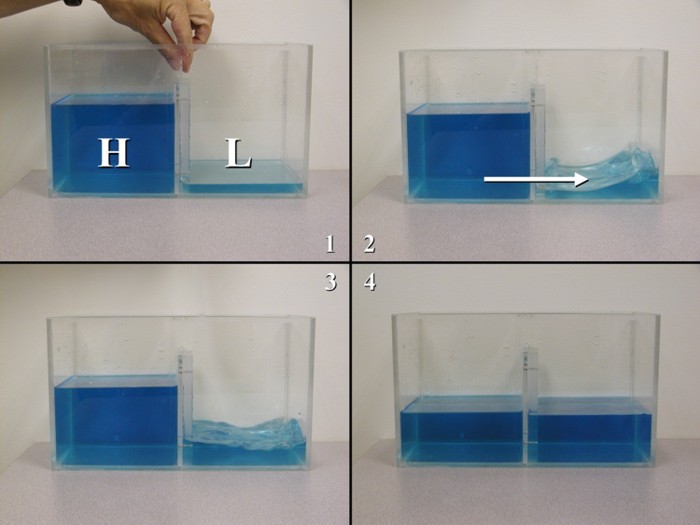
Isaac Newton's second law of motion states that when a net force is applied to an object, it accelerates; therefore, there must have been a net force acting on the water in order to set it into motion. In this case, the catalyst force was the pressure-gradient force, which acts from higher pressure toward lower pressure.
If the amounts of water in each compartment differ by a smaller amount, then the pressure-gradient force (PGF) is much smaller because the weights of the water in both compartments start out nearly the same. With a smaller pressure-gradient force, the flow of water will be much slower. Thus, we arrive at the following result: The magnitude of the pressure-gradient force (represented by the difference in water pressure across the partition in this experiment), dictates the speed of the flow of water.
In a sense, the atmosphere is like an "ocean of air," and switching our discussion from water to air gives the same result. Recall that the gradient of an atmospheric variable measures the difference over a given distance. So, if we're talking about the pressure gradient, we're measuring the difference in pressure over a certain distance. How do we assess the magnitude of the pressure gradient? You may recall that the pattern of isobars tells us how large or small the pressure gradient is:
- If isobars are packed very tightly (close together), that means there's a relatively large pressure change over a fixed distance, so the pressure gradient is large.
- If isobars are packed loosely (far apart), that means there's a relatively small pressure change over a fixed distance, so the pressure gradient is small.
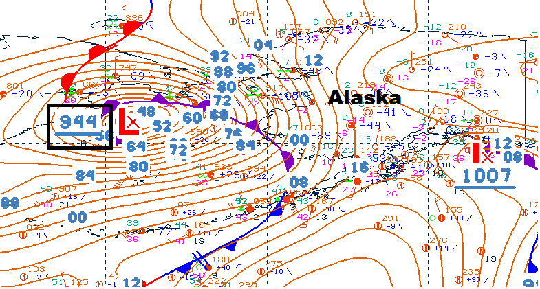
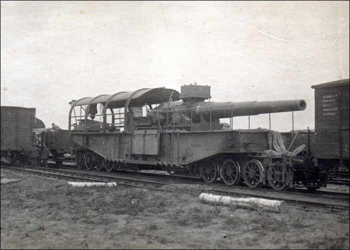
I should note that, mathematically, the values of most sea-level pressure gradients seem small. Even tight packings of isobars (equating to a "strong" pressure gradient force) ultimately amount to a change of a tiny fraction of a millibar per mile. Yet, when isobars are tightly packed, wicked winds can blow! For example, check out the seal-level pressure gradient around the extremely strong 944-mb low-pressure system over the Bering Sea on November 9, 2011 (see 06Z surface analysis below). The pressure-gradient force caused winds to really whip, as you can tell from this YouTube video from Nome, Alaska [17] (winds gusted over 50 miles per hour for several hours).
So, identifying areas with a relatively strong pressure-gradient force is as simple as finding areas on a map of sea-level pressure with where isobars are packed closely together. But, in what direction does the pressure-gradient force act? On maps of isobars, the pressure-gradient force is always directed perpendicularly to the isobars, and is directed from high to low pressure.
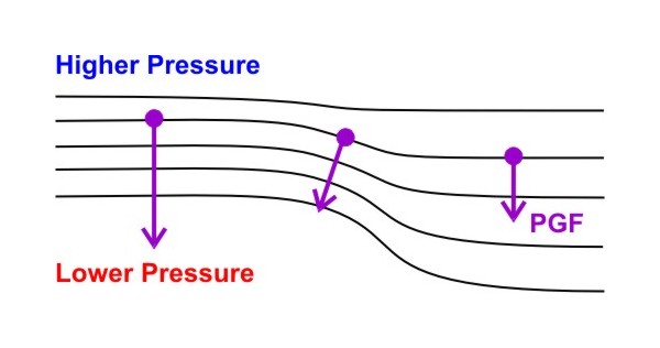
To see what I mean, check out the idealized surface weather map below. Ultimately, the pressure-gradient force has both a magnitude and a direction, so it's drawn as a vector that points from high to low pressure. Note how the orientation of the vector changes depending on the orientation of the isobars, but the pressure-gradient force always points perpendicular to local isobars, from higher toward lower pressure. The magnitude of the force is depicted by the length of the vector; note how the vector is longer where the isobars are packed closer together, indicating a stronger pressure-gradient force.
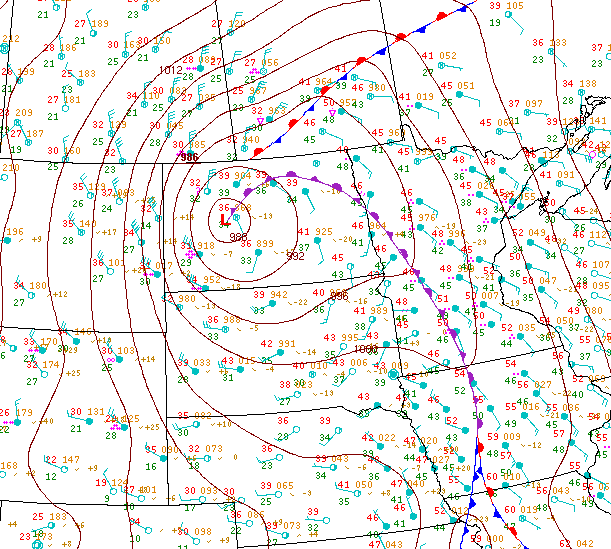
So, when isobars are packed closer together, the wind should blow faster, as the data from the intense low over the Bering Sea on November 9, 2011, indicate. The 12Z surface analysis from April 30, 2011 [18] provides another good example. First, note the 40-knot sustained winds over eastern Montana and western North Dakota compared to the 10-15 knot sustained winds over eastern North Dakota (where the isobars are packed more loosely). You should also notice that the winds aren't blowing directly perpendicular to the isobars, from higher pressure to lower pressure. What's up with that?
The wind would blow directly from higher to lower pressure if the pressure-gradient force was the only force acting on the air, but that's not the case. We have to account for other forces as well when trying to assess wind direction and speed. We'll examine another one of those forces up next. Read on.
Apparent Forces Have Real Impact
Prioritize...
At the completion of this section, you should be able to discuss the meaning of an "apparent force" and how apparent forces are created. You should also be able to discuss the Coriolis force, specifically what causes it, what determines its magnitude, what its effects are, and the time/space scales on which its effects are visible (and not visible).
Read...
Perhaps the title of this section has you a bit puzzled. What exactly is an "apparent" force? Well, "real" forces like the pressure-gradient force, can cause motion. But, we perceive some forces because of motion (these are "apparent forces"). Yes, perception is important when it comes to apparent forces, and to see what I mean, check out this time lapse of the sky over Penn State's Beaver Stadium from August 21, 2017 [19]. After a vibrant sunrise, you can watch the sun move across the sky. To us here on Earth, it looks like the sun is moving. But, is that what's really going on? Of course not! The earth revolves around the sun, and we're the ones moving, not the sun.
So, even though we perceive the sun moving across the sky, it's a false perception that arises from our frame of reference. By frame of reference, I mean the part of your immediate surroundings that you sense is not moving. Indeed, if you're standing still on earth, you perceive that you're not moving, but you're really flying through space at about 10,000 miles per hour along with the earth!
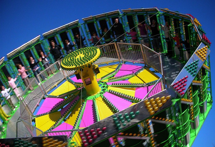
Our frames of reference give rise to "apparent" forces, too. For example, did you know that you accelerate every time you drive around a curve in a car (even if you keep your speed constant)? Acceleration, by definition, is a change in in a velocity vector, which means any change in speed or direction is an acceleration. There's an acceleration toward the center of the curve, but you perceive that your car is not accelerating as it negotiates the curve at constant speed. This perception leads you to falsely sense that some force, which acts to pull your body outward, is at work (more so if you're going too fast around the curve). But, this outward-accelerating force, called the "centrifugal force," is only an "apparent" force that arises from the false impression that the car's interior is not accelerating. If you've ever gone on a "tilt-a-whirl" type of ride at an amusement park (like the one below) you've felt the centrifugal force at work!
So, the fact that we falsely sense that our earthly surroundings are unaccelerated has big impacts for how we perceive the world around us, and that's a big issue when it comes to assessing the movement of air. Specifically, an apparent force, called the "Coriolis force" has a real impact on our observations of the direction of the wind.
Coriolis Force
Remember that I demonstrated the consequences of the pressure gradient force using a two-compartment water tank [23]. In that experiment, water flowed directly from high to low pressure over a short period of time. Air behaves much the same way on small time and spatial scales (for example, letting the air out of a balloon). On the much longer time scales and much larger spatial scales of high and low pressure systems, air does not flow directly toward low pressure. For example, check out the 18Z surface analysis on September 8, 2011 (below). Focus your attention on the closed, circular isobars and the wind barbs around Tropical Storm Lee (its center was just off the central coast of Louisiana at this time). Note that the winds don't blow directly toward the lowest pressure located at the center, so the pressure-gradient force must not be the only force at work.
What is this mysterious force that prevents air from moving directly inward toward the center of lowest pressure? It's the Coriolis force, which, like the centrifugal force, is an "apparent" force. Indeed, the Coriolis force arises simply as a consequence of the eastward rotation of our spherical earth. The Coriolis force is named after the French engineer and mathematician, Gustave Coriolis [25], who actually didn't study the effects of the rotating earth at all. He noticed the apparent force that would later be named after him during his work with rotating parts of machines.
So, how does the Coriolis force come into play in the atmosphere? Let's consider two points [26] at the same longitude, one at latitude 40 degrees north (we'll call Point N) and the other at 20 degrees north (Point S). Because the latitude circle at 40 degrees north is noticeably smaller than the latitude circle at 20 degrees north, Point S must move eastward faster than Point N because it must travel a greater distance around the equatorial circle during one 24-hour revolution of the earth. Indeed, Point S moves at approximately 900 miles per hour, while, at 40 degrees North latitude, the eastward speed of Point N (and all other points at 40 degrees north) is about 800 miles per hour. For sake of reference, the eastward speed at the North Pole is zero.
Peculiar things happen when points on the earth's surface move at different speeds as the planet rotates on its axis. Suppose a projectile is launched directly northward [27] from the equator toward latitude 40 degrees north. The projectile retains its great eastward speed as it starts its northward journey. With each passing moment, the northward-moving projectile moves over ground that has an eastward speed less than its own. In effect, the projectile surges east ahead of the lagging ground below. To an observer on the launching pad [28], the projectile appears to swerve to the right as a natural consequence of our spherical, rotating earth.
Launching the projectile from north to south results in a similar rightward deflection relative to the observer on the launching pad at 40 degrees north. The projectile, by retaining much of its original eastward speed of about 800 miles an hour, moves progressively over ground with faster eastward speed. In effect, the projectile falls behind the ground below, lagging increasingly to the west. To the observer on the launching pad at latitude 40 degrees north, the projectile again appears to deflect to the right. The bottom line is that no matter what direction the observer launches the projectile, the deflection will always be to their right in the Northern Hemisphere. I can make similar arguments for the Southern Hemisphere by first noting that if an observer in space looks "up" at the South Pole, the sense of the Earth's rotation appears to be clockwise [31], which is the opposite of the counterclockwise sense an observer gets while looking "down" at the North Pole. You can contrast the two in this animation showing each perspective [32]. Thus, deflections due to the Coriolis force in the Southern Hemisphere are to the left of the observer.
I've used an object moving north-south to demonstrate the impacts of the Coriolis force because I think it's the easiest to visualize. But, rest assured, Coriolis deflections to the right in the Northern Hemisphere (left in the Southern Hemisphere) occur regardless of the direction of motion. Coriolis deflections even occur for objects moving due east or due west, but I'll spare you the explanation (it's more abstract and harder to visualize than the north-south case).
Coriolis Force Effects (and Myths)
I emphasize that the Coriolis force is not a true force in the tradition of gravity or the pressure gradient force. It cannot cause motion. Rather, it is an apparent effect that simply results from an object moving over our spherical, rotating planet. The Coriolis force does not discriminate, either. Indeed, no free-moving object, including wind and water, is exempt from its influence. Given enough time, the Coriolis force causes air to move 90 degrees to the right of its initial motion caused by the pressure-gradient force. So, that means instead of air parcels crossing isobars directly from higher to lower pressure (as would happen if the pressure-gradient force was the only force acting), the combination of the Coriolis force and the pressure-gradient force causes air to move parallel to local isobars, counterclockwise around low pressure and clockwise around high pressure in the Northern Hemisphere (as depicted by the air parcel traces in the idealized weather map below). In the Southern Hemisphere, the circulation around highs and lows is reversed (it's clockwise around lows and counterclockwise around highs).
However, the magnitude of the Coriolis deflection depends on a number of factors. These factors depend on 1) the latitude of the moving object, 2) the object's velocity, and 3) the object's flight time. Its impact on air movement is clear because air moves over long distances for long periods of time. But, what about the impact of the Coriolis force on shorter events that happen on smaller scales? You may have heard that the Coriolis force determines the rotation of water swirling down a drain, or perhaps you've heard that the Coriolis force has a big impact on sporting events (like a baseball thrown from the pitcher's mound to home plate). Are these things true?
To begin to answer these questions, let's see how these three factors impact the magnitude of the Coriolis force:
- the magnitude of the Coriolis force increases with increasing latitude (closer to the poles) and is zero at the equator.
- the magnitude of the Coriolis force increases with increasing velocity of the object (or air parcel)
- the magnitude of the Coriolis force increases with increasing flight time (for the velocities typically observed in nature, a flight time of minutes to hours is typically required to observe any deflection at all)
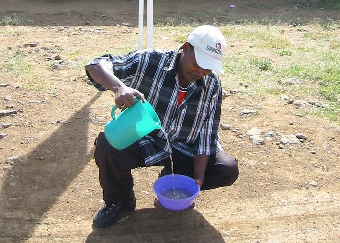
So, what's the upshot of these factors? Well, you typically cannot observe the Coriolis deflection of water emptying from a drain (the speed is too slow and the time is too short), for starters. This is also true of water swirling down a toilet bowl. Water circulates in a certain direction because the basin is designed to move water in that direction (as the case for toilets) or the swirling water is simply residual motion left-over from filling the basin. I point to these specific examples because they are often misunderstood in popular culture. Many videos on the Internet claim to show the Coriolis Effect via water draining out of a basin, such as this video taken in Equatorial Kenya [33]. This "experiment" has numerous problems (like using a different bowl in each case, for example), but the water draining from these small bowls occurs over too short a time for the Coriolis force to have a noticeable effect. Furthermore, at very low latitudes (right near the equator), remember that the magnitude of the Coriolis force is practically zero! Such video demonstrations are full of nonsense and bad science.
What about objects that move faster? I'll spare you the math, but let's see what the Coriolis force does to a 100 mph fast ball thrown from the pitcher's mound to home plate at Citizen's Bank Park in Philadelphia, Pennsylvania (near 40 degrees North latitude). At that speed, it takes the pitch about 0.4 seconds to reach home plate. Using these values, the Coriolis deflection is only 0.39 millimeters (0.015 inches)! That's far too small for anyone to see with the naked eye (or for any hitter to try to account for). How about a bullet fired at a long-distance target from a competition rifle? If we assume we're at 40 degrees North again, a bullet traveling 800 meters per second over a distance of 1,000 yards (0.57 miles) would have a flight time of 1.14 seconds and a Coriolis deflection of just 2.22 inches.
The "take away" point here is that although the Coriolis force affects all free-moving objects, these affects can be really small (perhaps undetectable), unless the speeds are very great or the travel time is long. The atmosphere has the advantage when it comes to the latter because air moves over long distances for long periods of time, and the Coriolis deflection becomes significant over the course of hours or days. So, when estimating wind direction we will need to consider both the pressure-gradient force as well as the Coriolis force. But, there's one more force that has important impacts near the surface of the earth that we have yet to tackle. Read on.
Against the Wind
Prioritize...
When you've finished this section, you should be able to describe the impacts of friction on wind speed, as well as describe the magnitude of the frictional force given a particular terrain.
Read...
So far, we've covered the main force that causes the wind (the pressure-gradient force), and the Coriolis force, which is an apparent force that arises because of the movement of air over our spherical, rotating earth. But, we have one more important force to cover in order to really get a handle on how the wind blows, and it's a force you're probably familiar with from other aspects of your life -- friction. In short, friction is a force that resists motion. If you try to "skate" across a floor with shoes on, you'll quickly realize it doesn't work very well because friction between the bottom of your shoes and the floor stops your feet from sliding easily. When driving, friction between your tires and the road helps you maintain control of your vehicle as you go around a curve. So, friction is a very important force!
How does friction impact the movement of air? Well, like the title of the 1980 Bob Seger song [37], friction is a force that works "against the wind" near the surface of the earth. I'll start by showing a quick example that I think will make the point. Below is an analysis of surface winds around Hurricane Irma as it was making landfall in southwest Florida around 21Z on September 10, 2017. The shadings denote wind speed, with darker oranges indicating faster winds. The arrows indicate the general direction of air movement (which is counterclockwise around the center of the storm).
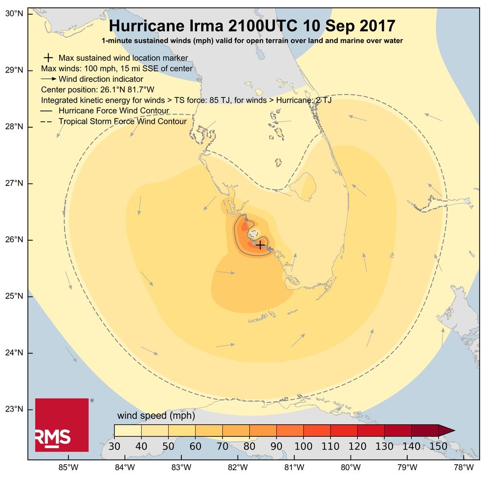
If you look closely, you'll notice that there's an abrupt drop in wind speed over Florida compared to over the surrounding water. This decrease in wind speed over land is evident not only near the center of the storm (just north-northwest of the "+" sign), but throughout Irma's entire wind field. Also, note how the abrupt decrease in speed closely mimics the shape of Florida's coastline. Near the coast of southeast Florida, for example, winds were blowing at 50 to 60 miles per hour over the waters of the Atlantic, but only 40 to 50 miles per hour on land. Without reservation, this rather abrupt reduction in wind speed was a consequence of friction over rougher land.
It may not be intuitive to you that air in motion near the earth's surface is slowed by friction. After all, at slow wind speeds, friction between the air and the ground (or other objects like trees and buildings) is indeed rather small. But, once the pressure-gradient force puts air in motion, collisions between air molecules and the stationary, rough ground cause the air to slow down a bit. So, when the wind blows, friction at the earth's surface acts to produce a wind-speed profile that increases with height because air right near the earth's surface is slowed the most by friction. The effects of friction decrease with increasing height above the ground, leading to faster wind speeds with increasing height (all else being equal).
So, what determines the magnitude of the frictional force? For starters, the magnitude of the force of friction increases with increasing speed: the faster surface winds blow, the greater the force of friction. The magnitude of friction also depends on the "roughness" of the surface. For example, air blowing across the flat plains of Kansas will encounter much less friction than, say, air crossing the rugged Rocky Mountains. Wind blowing over water (oceans, lakes, etc.) encounters the least amount of friction. The difference in friction over land versus water explains the abrupt decrease in wind speed over land in the surface wind analysis for Hurricane Irma above. Wind speeds over land were slower because of stronger friction over the relatively rough land compared to over the open ocean waters.
But, friction doesn't just impact wind speed. It also impacts wind direction. Recall that given enough time, if only the pressure-gradient force and the Coriolis force were acting, air would flow counterclockwise, parallel to local isobars, around low pressure in the Northern Hemisphere.
In the analysis of sea-level pressure around Tropical Storm Lee from September 8, 2011 that I introduced in the previous section, you can clearly see the sense of counterclockwise circulation from the wind barbs around the center of low pressure. But, the winds aren't blowing parallel to local isobars as we would expect if just the pressure-gradient force and the Coriolis force were acting. In fact, winds (especially those over land, where friction is stronger) are crossing isobars in toward lower pressure somewhat. For a better look, I've drawn some wind arrows [38] over the northern half of the storm to better highlight the fact that the wind is crossing the isobars in toward lower pressure somewhat.
Ultimately, friction was the main reason why the winds were crossing the isobars as they circulated counterclockwise around the center of low pressure because friction disrupts the balance that develops between the pressure-gradient force and the Coriolis force. We'll talk more about that in the next section, and put together all the forces we've covered to help you make judgments about wind direction and speed. Read on!
Getting a Handle on the Wind
Prioritize...
At the end of this section you should be able to describe how the pressure-gradient force, the Coriolis force, and friction act to determine the wind direction and speed. You should be able to define the geostrophic wind, and be able to determine the geostrophic wind and surface wind directions given a map of sea-level pressures.
Read...
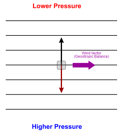
Now that we've learned about all of the forces that play a role in determining the speed and direction of the wind, let's see how they all work together. Ultimately, the air's motion depends on the sum of the forces that act on it, so to examine the movement of the air we'll consider a sample "parcel" of air released in a uniform pressure field in the Northern Hemisphere, and examine how each force impacts the air parcel. To do so, we'll look at this interactive force diagram [39] (keep the window open for the duration of our discussion), which will help you see the effects of adding various forces to a parcel of air. By convention, I'll use arrows to keep track of the pressure-gradient force, friction, the Coriolis force, and the parcel's velocity.
When you first open the interactive force diagram, only the pressure gradient force (PGF) is acting (the Coriolis force and friction are turned off. Leave it that way for now). Change the magnitude of the pressure-gradient force and watch how the spacing of the isobars changes. Also notice that the parcel's velocity increases (the velocity arrow gets bigger) as the pressure-gradient force increases. Conversely, the velocity decreases as the pressure-gradient force decreases. At this point, the velocity vector points northward, blowing directly from higher to lower pressure [40], which is unrealistic, because we know other forces are at work.
Now let's add the contribution of the Coriolis force (make sure friction is "off"). Remember that the Coriolis force depends, in part, on latitude; its magnitude is relatively small at low latitudes and relatively large at high latitudes. Select the latitude where you want the action to take place by moving the marker up (higher latitude and larger Coriolis force) or down (lower latitude and smaller Coriolis force). With both the pressure-gradient force and the Coriolis force acting on the parcel, you can see that the forces exactly balance each other, and the air parcel now moves parallel to the isobars with low pressure to the left of the direction of motion (again, we're assuming we're in the Northern Hemisphere).
This balance between the pressure-gradient force and the Coriolis force is called geostrophic balance, and the wind that results is called the geostrophic wind. But, how does geostrophic balance develop? I won't focus on the details, the process goes something like this:
- As the air parcel accelerates in response to the pressure-gradient force, the magnitude of the Coriolis force also steadily increases because the magnitude of the Coriolis force increases as speed increases.
- As a result, deflections to the right become greater with time, with the Coriolis force acting 90 degrees to the right of the (continually changing) direction of motion.
- The parcel curves toward the right until the magnitude of the Coriolis force balances the pressure-gradient force (geostrophic balance), and the parcel moves parallel to the isobars with lower pressure on the left of the direction of motion. This state of geostrophic balance is what's depicted on the interactive force diagram (and shown on the right).
The atmosphere is constantly striving for balance, and in geostrophic balance, there is no net force acting on the air parcel (because the pressure-gradient force and Coriolis force balance each other). Therefore, (according to Newton's laws of motion) the parcel will cease its acceleration and continue to move in a fixed direction at a constant speed. In this case, the final direction of the air parcel is directly eastward (in other words, the wind blows from the west), but in general, the geostrophic wind blows parallel to local isobars. Regardless of the strength of the pressure-gradient force (you can try varying it in the interactive force diagram), the end result is geostrophic balance, with a stronger pressure-gradient force leading to faster wind speeds.
I should point out, however, that the geostrophic wind is an idealized wind. It never perfectly occurs in nature. As you know, near the surface of the earth, friction is a factor (which we're about to get into) that disrupts geostrophic balance. However, the real atmosphere is often very close to geostrophic balance at high altitudes, where friction becomes negligible. So, we could look at isobars on an upper-air weather map and immediately get an idea of the wind direction by always remembering that the geostrophic wind blows parallel to the isobars. Knowing that narrows down the possibilities for wind direction to essentially two choices. But, if you imagine standing on the map with the geostrophic wind at your back, low pressure should be on your left in the Northern Hemisphere, which will allow you to find the correct wind direction.
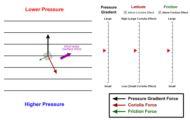
Near the surface, however, we have to deal with friction, so let's add it on the interactive force diagram. Make sure that the pressure gradient, Coriolis, and frictional forces are all turned on so that we can simulate real conditions on a surface weather map and observe the magnitude and the direction of the surface wind. Notice that the wind velocity vector got smaller (because friction slowed the wind speed) and now the wind blows across isobars in toward lower pressure somewhat [44]. If you imagine standing with the surface wind at your back in the Northern Hemisphere, low pressure is still on your left, but on average, it will lie about 30 degrees clockwise from your left arm (as shown above on the right). By the way, these "rules" are known in meteorology as Buys Ballot's Law [45].
Even with friction in the mix, the forces still achieve balance. Again, I'm going to skip some of the details of how the balance is achieved, but the process basically works like this:
- friction acts to slow a moving air parcel, which reduces the velocity
- with the parcel moving slower, the magnitude of the Coriolis force is also reduced a bit
- with the Coriolis force a bit weaker than it was in a geostrophic case, the pressure-gradient force is a bit stronger than the Coriolis force, which pushes air parcels across local isobars in toward lower pressure (alternatively, away from higher pressure).
So, ultimately, both friction and the Coriolis force work to oppose the effects of the pressure gradient force, but eventually a balance develops between the three forces and the parcel moves at a constant direction and speed. The bottom line is that the final path of the parcel takes it across the isobars inward toward lower pressure and away from higher pressure.
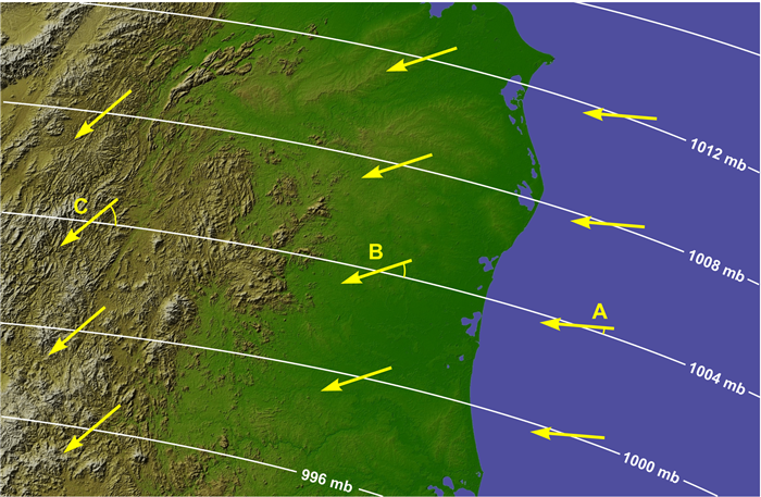
The angle at which a parcel crosses local isobars is determined largely by the magnitude of friction, and as you'll recall, friction depends on the velocity of the parcel as well as the roughness of the surface. Over land, the wind crosses the isobars at approximately 30 degrees, on average. Over the ocean and Great Lakes, the crossing angle (the angle at which the wind crosses the isobars) is generally less than 30 degrees, owing to less friction over usually smoother water (compared to rough land). Essentially, with less friction, the wind over the water is a bit closer to geostrophic than it is over land. In mountainous areas, where the effects of friction are greater, the crossing angle can be 45 degrees or even more. The difference in crossing angles can frequently be seen on weather maps (like the idealized map below).
It's the combination of the forces you've learned about that give rise to the counterclockwise flow around areas of low pressure (and clockwise flow around areas of high pressure) that you've seen on surface weather maps, like the sea-level pressure analysis from 18Z on September 8, 2011 [46] that I showed previously. In order to help you visualize the movement of air on maps of sea-level pressure, I created a couple of short videos that I think will help summarize the concepts we've covered, and help you determine wind direction from a map of isobars. The first video (1:46) will help you see how air parcels move depending on which forces are acting on them.
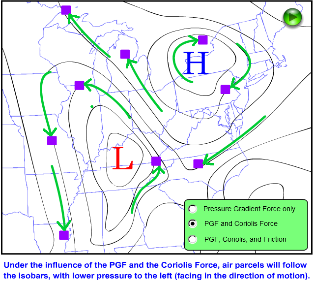
Let’s examine that paths air parcels will follow on this idealized weather map, based on the combination of forces acting on the parcels.
We have a map of sea-level pressure here, with an area of low pressure marked and an area of high pressure marked.
For our first case, we’ll pretend that only the pressure gradient force is acting on air parcels, which are marked by these purple boxes. If only the pressure gradient force acts, air parcels cross isobars perpendicularly, flowing from higher pressure toward lower pressure, like this
Now, let’s add in the Coriolis force. If only the pressure-gradient force and the Coriolis force act on air parcels, they’re in a state of geostrophic balance, and the Coriolis force turns the air parcels 90 degrees to the right of the original direction of motion in the Northern Hemisphere. So, air parcels in geostrophic balance flow parallel to local isobars, with lower pressure on the left of the direction of motion. You can also see the general counterclockwise flow around the low pressure, and the clockwise flow that results around highs.
Now, let’s add in friction, for the most realistic look at how air really flows near Earth’s surface. Friction disrupts geostrophic balance by slowing down the air parcels, which weakens the Coriolis force slightly. Eventually a balance develops between the pressure-gradient force, the Coriolis force, and friction, with parcels now crossing local isobars in toward lower pressure as they flow counterclockwise around lows and clockwise around highs.
To see the process of determining wind direction on a real map of sea-level isobars, check out the short video (3:09) below, in which I walk through a "recipe" for determining wind direction.
One of the objectives from the lesson, and a really useful skill, is to be able to look at a map of isobars and estimate the wind direction at any given point. And using the concepts from the lesson, we can do that. So I'm going to walk you through, kind of, the recipe that I go through when I need to estimate wind direction at a given point.
The first thing we have to do is we have to pretend that we're dealing with geostrophic winds. Now, with the geostrophic wind, we know that the pressure gradient force is exactly balanced by the Coriolis force. But in practical terms, the important thing about geostrophic winds is that they blow parallel to local isobars.
So at point A here, if we have winds blowing parallel to local isobars, they're either going to be from the southwest, or from the northeast. There's only two choices. So we have to determine which way they'd be blowing from.
And to do that, we have to remember our circulations around areas of high and low pressure. In the Northern Hemisphere, we have counterclockwise circulation around areas of low pressure, so that's going to give us a general sense of the wind flow that's like this. And that means that we have geostrophic winds that would be blowing from the southwest at point A.
Another way to think about it is that if you're standing with the wind at your back, lower pressures are going to be on your left. So if we stood with our wind at our backs at point A, and we were looking off toward the northeast, the only thing that makes sense is a southwesterly wind because that gives us lower pressures on our left. So geostrophic winds would be from the southwest, blowing parallel to local isobars at point A.
But we have to account for friction. The wind actually isn't geostrophic. Friction throws off the balance between the pressure gradient force and the Coriolis force, and it slows the wind down. But it also changes its direction and causes it to cross local isobars in toward lower pressure at a 30-degree angle, on average.
So if we take that into account, that means that the winds are going to cross the local isobars in toward lower pressure, about a 30-degree angle. And that's going to give us a wind that's almost from due south. Something around 180 degrees, give or take a little bit. So that's going to be our approximate wind direction at point A when we've accounted for friction as well.
We can do a similar analysis at point B. If we first pretend that the winds are geostrophic at point B, they're parallel to local isobars. So they're either from the east-northeast or from the west-southwest. And to figure out which one it is, we remember that air circulates clockwise around areas of high pressure in the Northern Hemisphere. So our general flow is going to be clockwise like this, and our wind flow is going to be from the east-northeast, parallel to these isobars. The geostrophic winds are going to be parallel to those isobars from the east-northeast.
But we have to account for friction, too. And to do that, we have to cross isobars at about a 30-degree angle away from higher pressure. So our winds would look something more like this, and ours winds would be from the northeast, or even north-northeast, at probably something like 20 or 30 degrees when we've accounted for friction because we don't actually have geostrophic winds.
Using the recipe described in the video above, you should be able to estimate the wind direction just about anywhere on a map of isobars, but I think it's important that you get some practice. Therefore, I've dedicated the next section to an activity that will help you refine this Key Skill. Read on!
Key Skill: Determining Wind Direction
Prioritize...
Using the interactive tool on this page, you should be able to apply the recipe given in order to estimate the geostrophic and surface wind directions at any point on a map of isobars.
Key Skill...
Being able to determine wind direction from a map of isobars is a key skill from this lesson. Make sure that you do not move on from this page without this skill. You can use the interactive tool below to practice applying the recipe for determining wind direction that I described in the video in the previous section:
- Start by figuring out the geostrophic wind direction. Remember that the geostrophic wind always blows parallel to the isobars, with lower pressure on the left (in the Northern Hemisphere). Remembering that winds flow counterclockwise around lows (and clockwise around highs) in the Northern Hemisphere helps, too. Note that the direction of circulation around highs and lows is opposite in the Southern Hemisphere because of the opposite orientation of the Coriolis force (so, flow around lows is clockwise and flow around highs is counterclockwise in the Southern Hemisphere). If you're finding the wind direction for an upper-level wind (not at the surface), this is all you need to do. Remember that wind direction is always given as the direction that it is blowing from.
- Next, if you are finding a surface wind direction, you need to take the geostrophic wind (which you just determined) and turn it inward toward lower pressure so that it crosses the isobars at roughly a 30-degree angle. Finally, don't forget to express the wind direction as the direction that it is blowing from.
Are you ready to practice? Using the map below, pick a point on the map and estimate the wind direction. To check your answer, hold down the left-mouse button over the location that you chose, and the local wind vector will appear along with the wind direction expressed in degrees. The orientation of the arrow represents the local wind direction, and the length of the arrow serves as a qualitative measure of wind speed. If you'd rather see the wind depicted as it would be on the station model, simply click on the Simulated Station Model in the menu below the surface analysis. This option will also give you a more specific sense of wind speeds, but the wind speeds are merely a reference. This tool does not actually calculate the real wind speed (it's a very complex calculation).
If you can consistently "predict" the correct wind direction at any point you choose on the map, you've got the hang of it, and you're ready to move on to the next section. Up next, we'll start exploring some of the weather "consequences" of patterns of surface winds.
Controlling Traffic Around Highs and Lows
Prioritize...
After completing this section, you should be able to define convergence and divergence and discuss the impacts of convergence and divergence (at the surface and aloft) on vertical motion, surface pressure tendency, and general weather conditions.
Read...
Recall from earlier in the lesson that surface air pressure can be closely approximated by the weight of an air column with a small fixed area that extends from the ground to the top of the atmosphere. Therefore, the center of a low-pressure system marks the air column that weighs less than any other column in the vicinity. But, our newfound understanding of how winds blow around low pressure at the surface (counterclockwise in the Northern Hemisphere, with winds crossing isobars in toward low pressure) presents a bit of a dilemma. If you look at the pattern of winds around Tropical Storm Lee [38] at 18Z on September 8, 2011, you can see that air essentially spirals inward toward the center of the low. This process of air "coming together" is called convergence.
Do you see the problem? As air spirals in toward the low's center, the mass of air columns near the center increases, thus making the weights of columns also increase. So, a surface low, by its own circulation, acts to increase pressure around its center, and thus ultimately causes its own demise. Seems sort of self-destructive, doesn't it?
Why would a low seemingly contribute to its own destruction? Think of the atmosphere as a place where there is a culture of "column peer pressure." In other words, there is a sort of atmospheric peer pressure at work that compels neighboring air columns to weigh about the same. How does this culture of column peer pressure work? Suppose there's an air column that's a bit of a lightweight (in other words, assume the air column lies over the center of a newly formed low-pressure system). The weight-conscious atmosphere immediately tries to add weight to this column by having surface air move toward this column. This general movement of air toward lower surface pressure is, very simply, the wind.
In a way, the culture of column peer pressure is similar to the cultures of human peer pressure. Such compelling peer pressure has the potential, when taken to extremes, to cause personal hardships (think about the negative consequences that peer pressure can have on school-aged children, for example). Column peer pressure, when taken to extremes, is no different! That's because column peer pressure, as you just learned, sets the stage for the wind to blow. When a low-pressure system rapidly develops and its central pressure drops like a rock, column peer pressure kicks into high gear, causing the wind to blow strongly toward the low's center. The fast speed of the wind is an attempt to compensate for the great weight loss in the air columns near the low's center. In turn, such strong winds can cause damage.
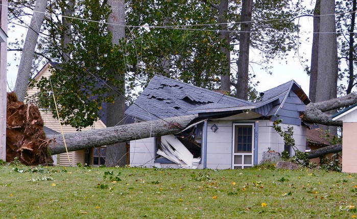
Sometimes, the strong winds associated with intense low-pressure systems can lead to unimaginable damage. The photograph above of destruction in the aftermath of Hurricane Ike strikingly proves my point. Ike was no longer a hurricane by the time it reached Indiana, but it was still a strong low-pressure system, and the effects of the accompanying winds were felt very far inland.
Just so I give equal time to highs, suppose that an air column is a tad on the heavy side (in other words, assume the air column lies over the center of a very modest high-pressure system). Remember that winds at the surface will flow clockwise around the center of the high (in the Northern Hemisphere), with winds crossing isobars away from the center of high pressure. Air essentially spirals away from the center of a high, and this process of air spreading apart is called divergence. With air moving away from the center of the high at the surface, the weight of local air columns decreases. Here again, the weight-conscious atmosphere generates the wind to shed weight from the heaviest columns near the center of the high.
So how do centers of high and low pressure maintain themselves for any length of time? Let's focus our attention on a newly formed low. The traffic jam of air (congestion, convergence of air, etc.) around the center of the low, which surely adds weight to local air columns, would prevent surface pressures from decreasing any further if acting alone. But, after most lows form, they don't start to die immediately. Indeed, most low-pressure systems reach maturity, attaining a central pressure much lower than the values they started out with. and I think an analogy will help you understand the corrective measures that lows take to manage extra weight they take on from convergence near the surface. Imagine a dollop of whipped cream sitting on a table top. If you were to smash the dollop by clapping your hands together (simulating convergence), the whipped topping would squirt upward (it can't squirt downward because the solid table just won't let it).
Though not as violent or as messy, the convergence of surface air around the center of a low promotes rising air (air can't go down because the ground just won't let it). Currents of rising air often lead to clouds and sometimes precipitation. Of course, this doesn't really solve the low's weight problem. Air moving upward in the column is still in the column, and its weight will contribute to the surface pressure (if you raise your hands while standing on a scale, you certainly don't weigh less). NOTE: Rising air does NOT cause low pressure. If you go searching around on the Web, you may very well find explanations that say that rising air causes surface pressure to decrease (or that low-pressure systems strengthen because of rising air). Not true!
So how does a low do it? A low-pressure system must compensate for the convergence of mass near the surface and shed that mass at high altitudes. Therefore, you will usually see a region of air diverging from the column over the center of a developing low-pressure system. As long as the low loses more weight at high altitudes than it gains near the surface, the total column weight will decrease, the surface pressure will decrease and the low will continue to develop.
The weight program for a high-pressure system is just the opposite. Rather than trying to maintain weight loss over a central column, a high pressure center must maintain the mass build-up that has resulted in a higher pressure than its surroundings. But, surface air diverges from the center of a high, thereby helping to lower column weight. Obviously, the atmosphere must take measures that allow column weights and surface pressures to increase at the center of developing high pressure systems.
To understand the measures that the atmosphere takes so that high-pressure systems can maintain their weight, let's return to my dollop of whipped cream on the table. To simulate the divergence of surface air, imagine dropping a book on the whipped cream. Sure enough, whipped cream squirts out horizontally (a messy form of divergence) as the book smashes down on the dollop. Though not as violent or as messy, sinking currents of air go hand in hand with the diverging low-level winds around a surface high-pressure system. Weatherwise, sinking air tends to cause clouds to evaporate, paving the way for dry, bright weather.
Of course, air sinking from higher up and then horizontally diverging near the earth's surface doesn't solve the high's weight problem. How does a body-building high maintain the weight of the air column at its center? As with the low pressure center, the key is to look for what's going on aloft. In the case of a developing high pressure system, more air converges or "piles up" in the column of air over the center of the high, offsetting the weight loss near the surface and allowing the column to undergo an overall weight gain. In turn, the surface pressure increases.
Summary
Surface pressure...
- decreases when weight is removed from air columns
- surface lows form and strengthen when the weight loss from divergence aloft is greater than the weight gain from convergence near the surface
- increases when weight is added to air columns
- surface highs form and strengthen when the weight gain from convergence aloft is greater than the weight loss from divergence near the surface
So, patterns of convergence and divergence (at the surface and aloft) are critical in determining trends in surface pressure. But, convergence and divergence at the surface doesn't just occur near the centers of lows and highs (respectively). Up next, we'll look at other features in the pattern of sea-level pressures that can help us identify zones of surface convergence and divergence.
Spokes of Highs and Lows
Prioritize...
At the completion of this section you should be able to define the terms "ridge" and "trough" as they pertain to surface pressure. You should also be able to discuss the patterns of surface convergence and divergence, as well as the vertical motion and typical weather associated with surface troughs and ridges.
Read...
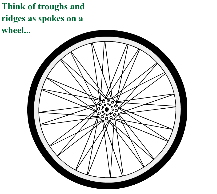
Like spokes on a bicycle wheel [49], there are "spokes" that extend outward from the hubs (centers) of low and high pressure systems, called "troughs" and "ridges." On the idealized surface weather map on the left below, the bulgings of the isobars south, north, east and west of the center of the low-pressure system are called troughs, which are simply elongated areas of low pressure. Instead of closed, oval-shaped isobars encircling a discrete center of low pressure, the isobars that form a trough are "open," with their cusps aligned to form a trough axis (the dashed lines running through the cusps in the isobars mark four distinct trough axes in the image below on the left).
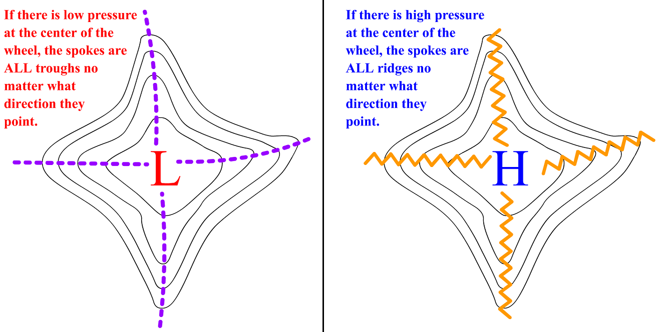
On the flip side of lows and troughs, spokes emanating from the center of a high-pressure system are called ridges of high pressure, which are simply elongated areas of high pressure. Instead of a few closed, oval-shaped isobars encircling a discrete center of highest pressure, the isobars that form a ridge are "open," with their cusps loosely aligned to form a ridge axis (the serrated lines running through the cusps in the isobars mark four distinct ridge axes in the image above on the right).
Troughs and ridges are key features to look for when examining a sea-level pressure map. Sometimes these features are easy to spot and identify, but other times identification can be tricky. Either way, you can always identify troughs and ridges by studying the pattern of isobars. For example, check out this idealized surface weather map [50], and focus on the low pressure system and its trough. Even if the center of low pressure wasn't labeled and the axis wasn't marked with a dashed line (the conventional symbol for a trough), we could identify southward bulge in the isobars as a trough by performing a simple check. Note that any two points A and B lying on opposite sides of the marked axis (at some small perpendicular distance) have pressures greater than the pressure of the corresponding point T on the axis. In this example, point T has a pressure of 1024 millibars, while points A and B likely have sea-level pressures of approximately 1026 millibars. Thus, the pressure at point T is a relative minimum. All points on the axis pass a similar test, so it's an elongated area of relatively low pressure, which by definition, is a trough.
Like the more compact closed-isobar centers of low pressure, troughs mark areas of convergence and rising air, making them potential breeding grounds for clouds and precipitation. To understand this claim, look at the wind direction following a single isobar (below) as it traverses the trough (all wind directions are consistent with previous discussions about the typical angles that surface winds cross isobars because of friction).
Note that, west of the trough axis extending south of the center of low pressure, winds blow from the west-northwest. East of the trough axis, winds blow from the south-southwest. It should be clear that trough axes always mark a shift in wind direction. Moreover, wind shifts at a trough axis are linked to convergence. As proof, picture the wind vectors as cars trying to round a sharp corner. In a trough, notice that each car is "cut off" by the car in front. Clearly, there is plenty of traffic congestion at the trough axis. In other words, there is convergence, and the air rises as a result.
In the real world, surface lows do not necessarily have four well-defined troughs that lie directly north, south, east and west of the low's center. Indeed, the number and orientation of well-defined surface troughs can vary from low to low. To see what I mean, check out this 15Z surface analysis from May 7, 2012 [51]. I've marked (with dashed orange lines) the troughs emanating from a pair of low-pressure centers. Just for the record, I removed the cold and warm fronts from the analysis just for clarity. It should be clear to you that surface troughs can extend in any direction (they certainly don't all sag southward).
In fact, when a trough extends northward, weather forecasters call it an "inverted trough." Sometimes, inverted troughs form north of developing low-pressure systems during the cold season. When they form over the Gulf States, inverted troughs have easy access to moist air overlying the Gulf of Mexico and are notorious for producing heavy precipitation as moist air converges and rises near the trough axis. In such cases, inverted troughs rank high on my list of big "weather makers."
Now let's turn our attention to ridges of high pressure. Remember that ridges are simply elongated areas of high pressure, and that's evident when you check out this idealized sea-level pressure map with a center of high pressure and associated ridge [52]. As with our trough above, we can perform a simple check to identify this northward bulge in the isobars as a ridge, even if the "high" wasn't labeled and the axis wasn't marked with a serrated line (the conventional symbol for a ridge). Let's choose any two points C and D lying on either side of the axis at some small perpendicular distance. Note that the point R that lies exactly on the axis has a surface pressure of 1020 millibars while air pressures at points C and D (about 1018 millibars) are less than at point R. Thus, the pressure at point R is a relative maximum. All points on the axis pass a similar test, so the axis marks an elongated area of high pressure, which is a ridge, by definition.
Like the more compact closed-isobar centers of high pressure, ridges of high pressure produce surface divergence. If we again draw wind vectors along a single isobar that traverses a ridge axis (like in the image below), note how air spreads out or diverges as it traverses the ridge. In compensation for surface divergence, air sinks in the columns of air located over the ridge axis, typically resulting in dry, bright weather.
Like troughs, the number, and orientation of well-defined ridges around a high pressure system varies from high to high. Here's a realistic example of a high-pressure system and its associated ridges [53]. Ultimately, weather forecasters are always on the lookout for surface troughs and ridges because of the implications for wind shifts, surface convergence and divergence, and rising or sinking air.
Summary
Surface troughs
- are elongated areas of low pressure
- are zones of surface convergence and rising air, often leading to clouds and precipitation
Surface ridges
- are elongated areas of high pressure
- are zones of surface divergence and sinking air, often leading to dry, fairly sunny weather
Troughs, in particular, are of great importance to weather forecasters because they also hold a connection to the air masses and fronts that we've studied previously. Read on to explore this connection!
Fronts and Pressure
Prioritize...
At the completion of this section, you should be able to discuss why fronts are located in troughs and discuss trends in sea-level pressure associated with a frontal passage.
Read...
Now that you've learned about the circulations around high- and low-pressure systems, we're going to tie that new knowledge in with some topics that we covered previously in order to help you better see the big picture. For starters, let's review a couple of key definitions:
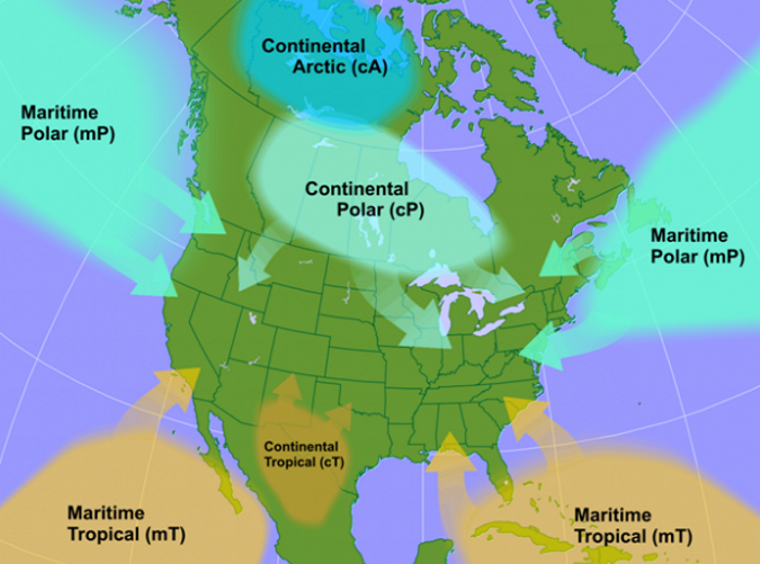
- Air Masses are large blobs of air with horizontal dimensions of several hundred to a couple of thousand miles, within which temperatures and moisture (dew points) at the surface (or at any other arbitrary altitude) are fairly uniform. In other words, temperature and moisture gradients within an air mass are small. Several types of air masses exist, and are named based on their source regions [54] (which determine their temperature and moisture characteristics).
- Fronts are boundaries that separate contrasting air masses. Since fronts lie at the edges of contrasting air masses, not surprisingly, fronts lie in zones with large gradients in temperature and dew point. The types of fronts we discussed previously are cold fronts, warm fronts, and stationary fronts.
So how are air masses, fronts, and the pressure pattern related? For starters, recall how air masses get their characteristics. In order for a large chunk of air to acquire the temperature and moisture characteristics of the underlying surface of the earth, it must stay over a given source region long enough for land or water to modify the overlying air. For this process to occur, it stands to reason that surface winds must be generally light. Broad regions of light winds are often found surrounding centers of surface high pressure, thus high-pressure systems mark the centers of air masses.
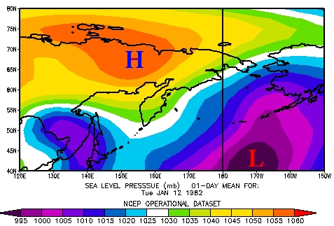
To see what I mean, check out the analysis of sea-level pressure from January 12, 1982 [55]. Note the strong high pressure system over Siberia, a region renowned as a source region for continental-Arctic (cA) air masses. Now, compare the pressure gradient around the high's center to the gradient around the low-pressure system centered over the Sea of Japan. Clearly, the pressure gradient associated with the high is much weaker than the pressure gradient around the center of low pressure, which translates to very light winds around the Siberian high. Those light winds allow the snow-covered, frigid ground to modify the overlying air and create a bone-chilling continental-Arctic (cA) air mass (the fact that northern Siberia, at latitudes above the Arctic Circle, tallies 24 hours of darkness each day during the heart of winter certainly helps).
So, if the "meteorological center" of an air mass is marked by a center of high pressure, then pressure must naturally decrease as you move toward the periphery of the air mass. When two air masses meet, the boundary must be a region of lowest pressure (because as you cross the boundary, pressure will start to increase again toward the center of another high). I think the schematic on the right, showing two opposing air masses and their high-pressure systems, provides a helpful visual. Clearly, the transition zone between the two air masses must lie in a region of relatively low pressure.
Of course, the boundaries that separate contrasting air masses are called fronts, which leads us to the following conclusion: fronts lie in troughs of low pressure. Now, not all surface troughs coincide with fronts, but the bottom line is that fronts naturally exist in elongated regions of low pressure (troughs). Also recall that surface troughs are regions of wind shifts and surface convergence. Therefore, since fronts lie in troughs, then it also stands to reason that shifts in wind direction and surface convergence occur along fronts.
Wind shifts along fronts are also supported by the notion that a front is a boundary between opposing high pressure systems. Notice in the diagram below that the flow of air associated with the two high-pressure systems is divergent -- spreading outward away from a center of high pressure. Along the stationary front (alternating blue barbs pointing toward warmer air and red circles directed toward cold air) that marks the boundary between the air masses, winds from markedly different directions meet. Ultimately, the stationary front lies just on the warm side of the large temperature gradient associated with the frontal zone (right).
The shift in wind direction, surface convergence, and the fact that fronts lie in troughs all have consequences for the weather you may experience when a front passes. To see what I mean, let's turn to the morning of February 14, 2015, when a cold front was passing through northwestern Ohio. You can see the location of the front on the 15Z surface analysis [56], and note how the front lies essentially between different areas of high pressure (contrasting air masses) similar to our schematics above. If we zoom in on the analysis [57], it becomes more apparent that the cold front also lies in a southwestward bulge in the isobars, which marks a surface trough. Also note the dramatic wind shift across the front -- southwest winds ahead of the front in eastern Ohio, compared to north-northwest winds behind it in northwestern Ohio, Indiana, and Michigan.
When the front passed Findlay, Ohio around 15Z, the change in weather was notable, as you can tell from the graphs below. The top graph plots temperature, dew point, and relative humidity from 04Z on February 14, 2015 through 05Z on February 15. I've marked 15Z with a vertical black line. At 15Z, both temperature and dew point (purple and green traces, respectively) started to decline as colder, drier air arrived behind the cold front (so temperatures started dropping, even though it was 10 AM local time). Winds (as marked on the station models below the top graph) shifted from southwesterly and west-southwesterly ahead of the front to northwesterly after the front passed.
Finally, the bottom graph shows sea-level pressure, and pressure reached a minimum around the time the cold front passed at 15Z. That should make sense to you, since fronts lie in troughs. Pressures steadily decreased until the front (and its trough) arrived, then pressure began increasing after the front passed (and the trough moved away with it). You can also tell that the frontal passage came with some snow (note the station model symbols for snow beneath the top graph), thanks in part to surface convergence and rising air in the vicinity of the front.
So, understanding the circulation of air around highs and lows, and how the pressure pattern ties in with air masses and fronts allows us to understand a lot of weather events that we experience! But, I've just scratched the surface here. We're just getting started in discussing the various types of weather (clouds, rain, snow, thunderstorms, etc.) that we experience every day. Specifically, this lesson has laid an important foundation, and we'll be applying many of its concepts during our look at low-pressure systems and the wide variety of weather that they bring (in the next lesson).