Lesson 11: Patterns of Wind, Water, and Weather in the Tropics
Motivate...

When you think of the tropics, or the word "tropical," you might picture white, sandy beaches, and perhaps sipping on a refreshing, fruity beverage (complete with a tiny umbrella in your glass, of course). Besides being a favorite vacation destination for many people, the tropics are home to some fascinating meteorology. One of the reasons locations in the tropics are such popular vacation destinations is a seemingly endless supply of sunny days and balmy breezes, but there's much more to tropical weather than that! In fact, some areas of the tropics are known for persistent rain (like rain forests that ring the equator).
Whether sunny or rainy, the hallmark of tropical weather is persistence. Weather patterns don't change much from day to day, and a big reason for the lack of variation is that the weather in the tropics is not dictated by the same driving factors as in the mid-latitudes -- namely temperature gradients. Cold fronts, warm fronts, and mid-latitude cyclones typically aren't found in the tropics because temperature gradients tend to be small overall.
Another curious characteristic of tropical weather is that winds tend to blow from only a few directions during the course of a year. Why is that? Based on what you've learned about the wind, the persistence of a few wind directions must mean that the pressure patterns don't change very much. So, fairly constant pressure patterns are present in the tropics (aside from the occasional tropical cyclone, which we'll cover in the next lesson) along with typically small temperature gradients.
In this lesson, we'll explore what causes persistent weather in the tropics, as well as explore the seasonal variations that do occur (some areas have a well-defined "wet season" and a well-defined "dry season"). We'll also explore the general circulation of the air in the tropics, which results in some of the tallest thunderstorms on the planet, as well as the driest deserts. We'll also discuss the Indian Monsoon and El Niño -- two of the more famous weather patterns in the tropics.
The tropics are full of "weather" that needs studying. So, pull up a beach chair and let's get started!
Meet the Tropics
Prioritize...
Upon completion of this section, you should be able to identify the meteorological region referred to as the tropics, be able to give context for its size (in relation to the entire earth), contrast typical temperature and pressure patterns in the tropics with those in the mid-latitudes, and discuss why the tropics are important energetically to the general circulation.
Read...
If we're going to study the tropics, we should start by defining exactly what the tropics are, but in reality, folks can't seem to agree on a single definition of the tropics. The definition from the glossary of the American Meteorological Society [4], for example, is pretty vague! Other definitions are based on geography, and define the tropics as the area between certain latitude lines in each hemisphere.
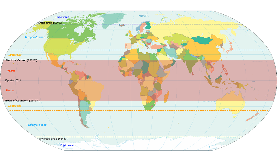
One common definition is to define the tropics as the area between the Tropic of Cancer (roughly 23.5-degrees North latitude) and the Tropic of Capricorn (roughly 23.5-degrees South latitude), highlighted in crimson in the image below. At some time during the year, the sun is directly overhead each point in this area. But, some definitions actually consider the tropics to cover a larger area, between 30-degrees North latitude and 30-degrees South latitude, given the similar climate characteristics which extend that far from the equator. This area (between 30-degrees North latitude and 30-degrees South latitude) actually accounts for exactly half of the Earth's surface! So, by this definition, the tropics are a pretty big area, and this large low-latitude region will be our focus when we talk about "the tropics."
The fact that the tropics receive more direct sunlight throughout the year than higher latitudes is the root cause of some of the curious characteristics of tropical weather, which make tropical weather quite different from weather in the middle and high latitudes. Consider these contrasts between the tropics and the middle latitudes, for starters:
- Seasonal swings in temperature across the tropics are typically small compared to the large swings that occur in the middle latitudes from summer to winter. In fact, temperature swings during the year in the tropics can be so small that the seasons are determined more by dramatic changes in clouds and rainfall.
- Wind directions in the tropics tend to be much less variable than they are in the middle latitudes (at many tropical locations, a single particular wind direction tends to dominate) because of persistent pressure patterns.
- Tropical cyclones (which we'll cover later) tend to form and thrive over warm, tropical seas with small horizontal temperature gradients. Meanwhile, you've learned that mid-latitude cyclones thrive off of large horizontal temperature gradients.
We'll explore these throughout the coming lessons, but for now, also consider that the intense solar heating over the low latitudes of the tropics throughout the year has consequences for global energy balance, as well. To see what I mean, check out the short video (2:21) below.
As discussed in the video, the relatively large losses of infrared energy to space over the tropics only partially offset strong solar heating, resulting in a broad surplus of energy that varies little with latitude between 30 degrees North and South latitude. This relatively even distribution of surplus energy across the tropics accounts, in part, for the general lack of moderate to large horizontal temperature gradients in the tropical troposphere.
One other reason for the generally small temperature gradients at low latitudes is that water covers approximately 75 percent of the tropics. That means the uniform surplus of energy in the tropics gets distributed over large expanses of water, thus further limiting opportunities for large temperature gradients to form (cold air traveling over relatively warm ocean waters gets rapidly modified).
The figure above represents the long-term average of annual surface air temperatures across the globe. I point out that there are indeed temperature gradients between tropical land masses and surrounding oceans, but the overall pattern of temperature gradients in the tropics is weak compared to those at higher latitudes.
Now, I readily admit that any annual average in temperature tends to "wash out" strong signals of gradients in winter, so perhaps a look at temperatures for a single day would be more telling. Check out daily global surface temperatures for January 7, 2018 [9] (units are Kelvin [10]), when sharp temperature gradients existed over eastern North America, for example, on the fringe of a continental Arctic air mass. Now, compare them to the flabby gradients over the tropics. No contest, wouldn't you agree? Notice that there are some sharper gradients along the outer fringes of the tropics near 30 degrees north. These larger gradients near 30 degrees are not unusual, given that Arctic air masses drive farther south in winter (occasionally into the fringes of the tropics). In the heart of the tropics, however, gradients are small by any standard.
But, it's not just temperature gradients that are small in the tropics. Pressure gradients are small, too (aside from tropical cyclones). For example, check out the chart of average sea-level pressures at 00Z on February 12, 1998 [11] (units are Pascals; 1 Pascal = 100 millibars). At the time, there were intense northern hemispheric low-pressure systems over the Gulf of Alaska, the Great Lakes, the middle Atlantic Ocean, northern Russia and the east coast of Asia (splotches of blues and purples on the map). Meanwhile, robust high-pressure systems (bigger blobs of greens, yellows, oranges and reds) were interspersed between the intense lows. In the tropics, on the other hand, pressure patterns are much more relaxed and much more equable than the middle latitudes. In other words, prominent centers of high and low pressure are more difficult to find, especially equator-ward of latitudes 30 degrees north and south. The one exception was a spot of relatively low pressure (blue splotch) just to the east of Madagascar in the southwest Indian Ocean, which is the signature of Tropical Cyclone Ancelle.
Since the pressure gradient force is a primary driver of wind speed, you might think that the winds are almost always weak in the tropics (outside of tropical cyclones, that is), with the small pressure gradients that exist there. But, that's far from the truth! To help you visualize the fact that many places in the tropics are quite breezy, despite small surface pressure gradients, I'm going to introduce a type of plot called a "wind rose." Wind roses display the observed frequency of wind directions (and sometimes speeds) at a particular location. On the left below is a histogram displaying frequencies of observed wind speeds (in meters per second) at an ocean buoy moored at 8 degrees South, 95 degrees West [12] during the year 2002. On the right is the corresponding wind rose for the buoy, which shows the frequency of observed wind directions during the same year.
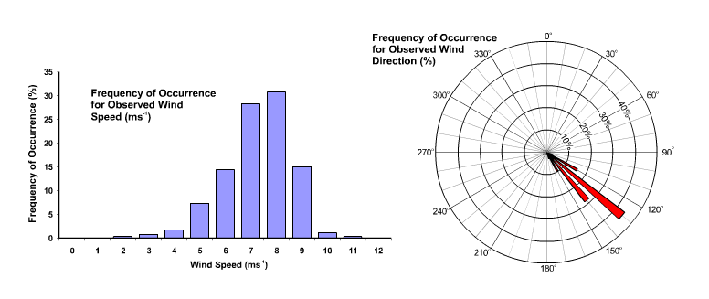
From these two images, we can quickly get two important messages. First, wind speeds at the buoy were between five and nine meters per second (roughly 10 to 20 miles per hour) the vast majority of the time, which hardly constitutes "weak" winds. Second, the direction from which the wind blew during the year was remarkably consistent. To get your bearings with the wind rose, note that each concentric ring represents a ten-percentage point increase in the relative frequency of the observed wind direction. Thus, the daily mean wind direction of 130 degrees (from the southeast) occurred on nearly 45% of the days, and the daily mean wind direction of 140 degrees occurred on about 28% of the days! The wind rose clearly demonstrates that winds retained their overall southeasterly direction for almost the entire year (and didn't deviate much from 130 degrees). Such consistency is in stark contrast to the middle latitudes, where the many high- and low-pressure systems that pass by during the year result in wind directions that are much more variable.
As you'll soon learn, persistent winds from the southeast (in the Southern Hemisphere tropics) and northeast (in the Northern Hemisphere tropics) are the signature of the reliable "trade winds." To start unraveling the mystery of these persistent tropical breezes, we have to start exploring how air circulates through the tropics. Not surprisingly, the direct solar heating in the tropics throughout the year again plays a critical role. Read on.
The General Circulation
Prioritize...
After completing this section, you should be able to define Earth's "general circulation," and be able to discuss the Hadley circulation in the tropics, specifically the Intertropical Convergence Zone (ITCZ) and the hot towers that form along it.
Read...
Astronomer Edmond Halley [13] loved to dabble in various scientific fields of study. In 1705, he calculated that a bright comet he observed in the heavens was periodic and that it would return in 1758. His computations were correct, although Halley didn't live long enough to see his prediction come true. In deference to his achievement, the comet now goes by the name Comet Halley. Besides astronomy, Halley also was into tides, cartography, naval navigation, and, yes, tropical meteorology. Halley actually offered the first detailed explanation of the trade winds, which were first discovered by Christopher Columbus on his voyage to the New World [14]. These reliable winds were so crucial to commercial sailing ships that the name "trades" developed. Ever inquisitive, Halley aspired to formulating a complete scientific theory that explained the trades.
In 1735, George Hadley [15] supported Halley's theory that strong solar heating over equatorial regions incited rising currents of air that eventually hit a ceiling of sorts (the tropopause) and then spread poleward, culminating in sinking air over latitudes much farther away from the equator. Envisioning a closed circuit of air (see the schematic on the right). Hadley saw the trade winds as the return (equator-ward) flow of air at low levels.
According to Hadley, these closed circuits (one in each hemisphere), which would eventually be called Hadley Cells in his honor, were part of his model of the earth's general circulation. What exactly is the Earth's general circulation? Suppose that winds at a given location are averaged over time periods longer than the longest-lived weather system (a season, for example). Often, a preferred speed and direction emerge. The global distribution of these "preferred winds" at a variety of altitudes constitutes the general circulation.
Hadley's model was somewhat oversimplified (especially at middle and high latitudes), but he had the right idea about the general circulation in the tropics. Indeed, the strongest signal in the earth's general circulation comes from the tropics, where the persistent Hadley Cells govern the monotonously persistent weather at low latitudes.
There are pronounced seasonal changes in the tropics, but these changes are not as closely linked to the sun angle as they are over the middle and high latitudes. Indeed, seasonal variations in temperature, which are usually small by mid-latitude standards, are somewhat out of step with the "solar calendar". Instead, they are often in step with seasonal shifts in wind direction or trends in precipitation. These seasonal shifts are largely governed by the location of the Intertropical Convergence Zone (ITCZ), which is the region where the opposing trade winds in each hemisphere converge. The annotations on the infrared satellite image below show idealized trade winds converging along the ITCZ.
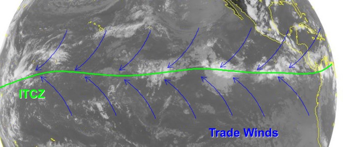
Note in the image above that tall, cumulonimbus clouds mark clusters of showers and thunderstorms along the ITCZ. Indeed, the ITCZ is typically marked by a broken chain of showers and thunderstorms that rings the globe as converging trade winds give warm, moist air parcels a nudge upward to initiate convection. Air rises in these so-called "hot towers" all the way up to the tropopause (which is at a higher altitude in the tropics than it is at higher latitudes) and spreads poleward, eventually sinking near 30 degrees North and 30 degrees South latitude. Some of that air then flows back toward the equator at the surface, forming the trade winds and completing the closed circuit of the Hadley Cells.
That's just a quick look at the basics of Hadley Cells in the tropics, but there are more details to explore. For example, the convergence in the ITCZ doesn't universally occur along the equator (the location of the ITCZ meanders throughout the year). Why is that? We'll find out as we explore the ascending branch of the Hadley Cell coming up next!
The Ascending Branch of the Hadley Cell
Prioritize...
When you're finished with this section, you should be able to discuss seasonal variations in the position of the ITCZ and their consequences for local weather and climate (precipitation, in particular). You should also be able to define thermal equator and doldrums.
Read...
If you're into "oldies" music, you might be familiar with the song "I'll Follow the Sun [16]" by The Beatles. As it turns out, this hit song could be the anthem of the Intertropical Convergence Zone (ITCZ) and the ascending branch of the Hadley Cells. By way of review, the Hadley Cells are closed circulations of air rising over equatorial regions, flowing poleward at high altitudes, and sinking and returning equatorward via the low-level trade winds. The ITCZ marks the region where trade winds from each hemisphere converge. This zone of convergence, as well as the Hadley Cells themselves, are a product of strong solar heating at low latitudes. But, the ITCZ isn't located right at the equator (as you might think). Why is that?
Recall that over the tropics, there's a net gain in energy over the course of a year because incoming solar radiation dwarfs radiation emitted from the tropics. Consider this image created by NASA that shows the net radiation distribution over the earth [17] during December 2001. The green shadings indicate surpluses in radiation, while blues indicate deficits. Clearly, the Southern Hemisphere (where it was summer) was running a surplus, while most of the Northern Hemisphere (where it was winter) ran a deficit. The tropics, however, run a surplus pretty much all year round, which you can get a feel for by watching this animation of net radiation distribution [18] from December 2001 to December 2002. In the animation, the low latitude regions that mark the tropics are always shaded in green (indicating a net gain in radiation).
Given the continuously large energy surplus at low latitudes, there is a zone of maximum heating called the thermal (heat) equator that exists. The thermal equator connects all the points that have the highest annual mean temperatures compared to other locations at their longitude. For the record, the thermal equator bears no relationship to the geographical equator. That's because mountain ranges, ocean currents, and differences in heating between continents and oceans naturally prevent a smooth, latitudinal variation in temperature in equatorial regions. The thermal equator lies mostly in the Northern Hemisphere, as the plot of mean annual temperature below shows, primarily because the Northern Hemisphere has more land at low latitudes (which, of course, becomes hotter than surrounding oceans with strong solar heating).
Furthermore, the thermal equator marks the average annual position of the ITCZ. Given the link between the ITCZ and high surface temperatures, the ITCZ lies in a trough of low pressure because high temperatures in the lower troposphere cause the air density (and weight) to decrease in local air columns, which, in turn, helps to promote lower surface pressure. Lower surface pressure is further promoted by the fact that air spreads out near the tropopause and flows poleward at the top of the ascending branch of the Hadley Cells. This upper-level divergence also helps reduce the weight of local air columns. Thus, analyses of sea-level pressure aid in finding the position of the ITCZ in real time (or over a given time period). For example, I drew the mean positions of the ITCZ during January and July using patterns of sea-level pressure as a guide below.
Note that in January, the ITCZ is mostly located in the Southern Hemisphere, where summer is occurring. But, the ITCZ drifts northward as the seasons change and is mostly located in the Northern Hemisphere in July (when it's summer in the Northern Hemisphere and solar heating is stronger there). On any given day, in response to maximum heating and low-level convergence, a ragged belt of cumulonimbus clouds fed by relative strong upward motion usually hangs like a necklace around the globe [19], marking the ITCZ.
I point out that, on any given day, the prevailing pattern of clouds associated with the ITCZ may not reflect a continuous belt of convection over equatorial latitudes, but tracking the rain that falls from showers and thunderstorms in the ITCZ can help us see how its position varies throughout the year. To see what I mean, check out this loop of monthly averages of rainfall [20] (estimated from satellites) in millimeters per day, that fell from January 1999, to January 2003. The strong signal of rainfall associated with the ITCZ and the ascending branch of the Hadley Cells should be apparent to you. Clearly, the ITCZ "follows the sun" as it drifts north and south along with the belt of maximum solar heating throughout the year.
Since the ITCZ coincides with a belt of low sea-level pressure, low-level air flows horizontally and converges toward the thermal equator as the atmosphere attempts to equalize the weights of air columns. Those converging winds are indeed the trades. Check out this cross section schematic [21] and note that the ITCZ corresponds with the ascending branch of the two Hadley Cells (one in each hemisphere). In case you're wondering, the background image was created by a down-looking LIDAR (a "light-equivalent" of radar that detects clouds) aboard the space shuttle Discovery. By the way, the zone where the opposing trade winds converge generally has light and variable winds. For this reason, this east-west belt is called the doldrums, which means "much rain and light winds".
How much rain falls in the doldrums thanks to the ascending branch of the Hadley Cells? Let's focus in on a particular area to see. If you recall the figure showing the January and July positions of the ITCZ [22], you can see that the there's not much of a seasonal shift over northwestern South America near the Amazon River Basin. Thus, a recurrent dose of rising currents of humid air characterizes this region. Indeed, check out the annual mean precipitation [23] over northern South America, which shows average rainfalls up to 3,500 millimeters (almost 140 inches) over the Amazon River Basin.
In regions where the position of the ITCZ varies more dramatically during the year (unlike the Amazon River Basin), a clear-cut wet and dry season emerge. Take, for example, the Brazilian city of Fortaleza [24], which is located on the northeast coast. In the animation below, you can review the monthly averages of rainfall and track the seasonal migration of the ITCZ with respect to Fortaleza on the inset map of global monthly precipitation. Note that the heavy rainfall associated with the ITCZ dips southward to Fortaleza's latitude and then retreats northward. This annual variation dictates that there are rainy and dry seasons at Fortaleza, as you can see from the bar graph of average monthly precipitation (late summer and fall mark Forteleza's dry season).
If you revisit the loop of monthly average rainfall from 1999 to 2003 [20], the blotches of white (indicating very little precipitation) that line up at latitudes near 30-degrees South and North also stick out as curious features. Ultimately, what goes up in the ascending branches of the Hadley Cells, must come down, and these dry regions correspond to the sinking branches of the Hadley Cells. We'll explore them in the next section. Read on!
Subtropical Highs
Prioritize...
On this page, you should focus on the cause of the belt of subtropical highs, and be able to describe their formation, strength, and seasonal changes based on column-weight issues. You should also be able to discuss the dominant vertical motion in the belt of subtropical highs and its implications for local weather and climate.
Read...
As you just learned, high over the Intertropical Convergence Zone (ITCZ), extra-tall cumulonimbus clouds prod and poke the tropopause on a regular basis. To hammer home the connection between the position of the ITCZ and the frequency of thunderstorms, check out this animation representing the average number of daily lightning flashes [25] from January 1 to December 31 (daily averages are based on satellite-based measurements between April, 1995, and November, 2000). Just based on the lightning frequency, you can follow the imprint of the ITCZ as it meanders north and south throughout the year, as well as identify the summer and winter hemispheres even though the individual dates aren't labeled.
Once rising air parcels reach the tropopause, its greater stability acts like a lid to suppress further ascent (remember that the air above the tropopause in the stratosphere is quite stable). So, upon reaching the lid, rising air parcels fan out laterally, heading poleward in both hemispheres and thus becoming part of the upper branches of the Hadley Cells. Parcels head toward the subtropics, where they will eventually sink in concert with the belt of subtropical high-pressure systems that girdles the globe at latitudes in the general vicinity of 30-degrees North and South. These "subtropical" highs form near the fringes of the tropics and are semi-permanent, meaning that they typically appear on long-term-average pressure patterns. To see what I mean, check out the long-term average of sea-level pressures from June through August (top image below) and December through February (bottom image below) to spot the subtropical highs.
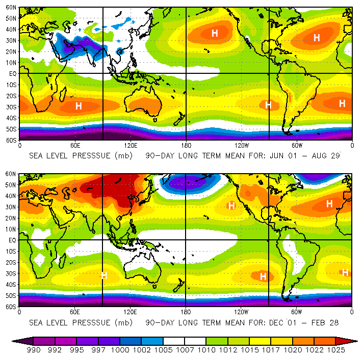
During summer in the Northern Hemisphere (top image above), two dominant subtropical highs emerge -- the Bermuda high over the Atlantic Ocean and the Pacific high. The Bermuda high shares its name with the island of Bermuda because, over the long haul during summer, the average position of this high lies near Bermuda. These two subtropical highs owe their relative strength, in part, to the oceans. During the Northern Hemisphere's summer, the oceans are generally cooler compared to the warmer continents. In turn, cooler, denser maritime air that overlies the oceans serves to boost surface pressures, paving the way for relatively robust subtropical highs during summer.
During the Northern Hemisphere's winter (bottom image above), when the oceans are warmer compared to the continents, the dominant subtropical highs aren't as strong, with the Bermuda high shifting eastward and gradually taking an average position near the Azores Islands. As a result, the Atlantic subtropical high assumes the seasonal name, Azores high.
So, why do these subtropical high-pressure systems exist in the first place? Over the long haul, the clear signal from the recurrent upward motion in the ascending branch of each Hadley Cell is a stream of air flowing poleward at high altitudes. As the air flows poleward it cools. And eventually, in the general neighborhood of 30-degrees latitude, the poleward flow in the upper branch of each Hadley Cell becomes convergent. In turn, this mass convergence of cold air moving in the upper branch of the Hadley Cell adds weight to local air columns near 30-degrees latitude, increasing surface pressure there, and helps to establish the persistent belt of subtropical highs.
To gain insights into how this high-level convergence occurs, check out the polar stereographic projection of the Northern Hemisphere below. In the image, I highlighted the equator and the latitude circle at 30 degrees for effect. Imagine moving a closed belt of high-altitude air situated over the equator all the way to 30-degrees latitude. There's little doubt that there has to be a "squeeze play." Thus, air must converge as it moves poleward from the equator.

The bottom line is that the mass convergence in the upper branches of the Hadley Cells increases column weight, and thus, surface pressure. It also promotes sinking air, which as you may recall, causes air parcels to warm as they compress because of increasing air pressure at lower altitudes. This sinking (and warming) air in and around the cores of subtropical highs actually works against the increase in column weight caused by upper-level convergence, serving as a "check" on the strength of the subtropical highs. The gently sinking and warming air also leads to increased stability over and east of the centers of the subtropical highs, which stifles the development of showers and thunderstorms.
Structurally, subtropical highs aren't merely "surface dwellers." To the contrary, there are reflections of the subtropical highs throughout most of the troposphere. Indeed, check out the spatial relationship between the surface Bermuda high and its reflections higher in the troposphere [26] at 12Z on September 1, 2003. This three-dimensional nature of the subtropical highs means that they influence wind patterns aloft, too, with their broad clockwise flow (in the Northern Hemisphere). Later, you'll learn that winds aloft play a key role in steering tropical cyclones, so it stands to reason that the upper-air reflections of the Bermuda high (and subtropical highs, in general) are important factors in steering tropical cyclones.
Besides acting as a back-seat driver for tropical cyclones, subtropical high-pressure systems provide another piece to the puzzle of weather and climate at low latitudes. Notable contrasts in precipitation exist between the domains of the subtropical highs (in the general neighborhood of 30-degrees latitude) and the wet equatorial zones. If you return to the movie of average monthly precipitation [27] from the last section, the white blobs near 30-degrees latitude mark areas where very little precipitation falls. Clearly, the broad areas of sinking air within the belt of subtropical high-pressure systems take their toll on precipitation, with the associated warming discouraging the development of clouds. As a result, the region of subtropical highs tends to be very dry. For example, the desert landscape of Monument Valley [28] (southeast Utah and northeast Arizona) is a result of an annual average precipitation only around five inches.
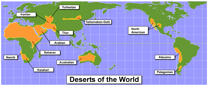
It's pretty much the same story through large swaths of the subtropics in both the Northern and Southern Hemispheres. Indeed, the hot land deserts of the world primarily lie within the persistent belts of sinking air associated with the subtropical high-pressure systems, as shown in the map below. The dearth of water vapor and the lack of vegetation over these deserts all but eliminates clouds to block the sun and evaporational cooling near the ground during the daytime, paving the way for high afternoon temperatures. At night, the dry, frequently cloudless atmosphere readily transmits infrared energy through the atmosphere, allowing for rapid cooling, and setting the stage for diurnal temperature variations of up to 50 degrees Fahrenheit or more!
Finally, I'll remind you that the Hadley circulation is the long-term average weather pattern over the tropics. Indeed, each Hadley cell is not a steadfast circulation that you can readily observe on a daily basis. For example, the Hadley circulation in the Northern Hemisphere's summer gets nearly obliterated by the intense, uneven heating of continents and oceans at low latitudes (the interruption of the Hadley circulation during the Southern Hemisphere's summer is noticeably less pronounced). Despite these summer interruptions, the relatively clear signal from the Hadley circulation becomes, over the long haul, a defining weather pattern at low latitudes.
For a complete summary of the Hadley circulation, here is a cross section of the Hadley Cells in both hemispheres [29], showing the ITCZ and the ascending branches, the poleward flow in the upper branches, sinking air in the subtropics and the corresponding subtropical highs, and, finally, the equator-ward return flow associated with the trade winds. Remember that the circulation is driven by strong solar heating, which ultimately manifests itself in a trough of surface low pressure that marks an elongated area of wind shifts (where the northeasterly trades meet the southeasterly trades). Air rises there in the ITCZ, and upper-level divergence below the tropopause helps keep surface pressures relatively low, helping to maintain the surface trough and the low-level convergence that helps to fuel the ascending branch of the circulation.
So far, we've focused on the ascending branches of the Hadley circulation in the ITCZ and the descending branches that form the subtropical highs. But, we haven't talked much about the upper and lower branches. When I briefly discussed the upper-branch above, I ignored the effects of the earth's rotation on the movement of air to create a simpler picture. But, when the Coriolis force is added to the mix, the upper branches of the Hadley Cells take a much more swirling route [30]. We'll explore the consequences of this swirling route toward the subtropics next. Read on!
The Subtropical Jet Stream
Prioritize...
Upon completion of this section, you should be able to discuss the formation and average location of the subtropical jet stream (STJ), its seasonal variations in intensity, and its impacts on mid-latitude weather.
Read...
Back when we studied mid-latitude cyclones, we talked a bit about the jet stream, which is a channel of fast winds near the top of the troposphere. But, the jet stream we talked about is really the mid-latitude jet stream, which regularly affects weather in the mid-latitudes. The mid-latitude jet stream isn't Earth's only jet stream, though!
In our discussion of subtropical highs, we ignored the earth's rotation and the Coriolis force when we discussed the high-altitude, poleward flow in the Hadley Cell [29]. Because our planet rotates, air doesn't flow directly toward the poles at high altitudes. Indeed, it takes a much more swirling route [30]. As air flows poleward in the upper branch of the Hadley Cell, eventually it curves toward the east (in the Northern Hemisphere). The end result is that air parcels in the upper branches of the Hadley Cells end up circling the earth during their lofty treks from equatorial regions to the subtropics. This poleward spiral culminates in the subtropical jet stream ("STJ", for short) near 30-degrees latitude.
The STJ was actually one of the last major tropospheric features to be discovered by direct human observation. During World War II, American pilots, while flying westward in the vicinity of Japan and other islands in the Pacific, reported ground speeds dramatically lower than the aircraft's indicated air speed. Flying at very slow speeds relative to the ground could have meant only one thing - one whopper of a headwind! Check out the image below, which shows the long-term-average wind speeds (in meters per second) and directions near 40,000 feet over Asia and the western Pacific Ocean during meteorological winter (December, January and February). The narrow ribbon of fast winds near latitude 30 degrees marks the average position of the STJ. Although pilots could make little headway on some of their missions, they had made a major discovery!
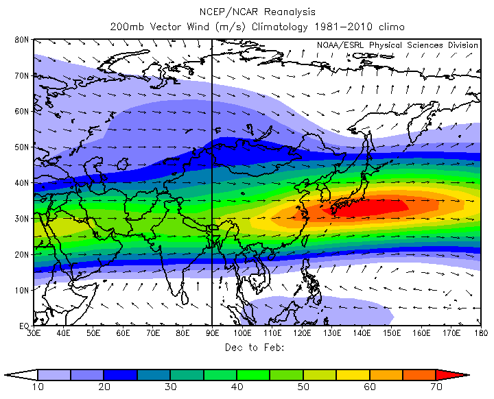
In fact, the STJ is stronger over the western Pacific region, on average, than any other place in the world. That's primarily because the Himalayan and Tibetan high ground interrupt and divert the generally westerly flow of air in the upper troposphere [31]. Farther east, diverted branches of air flow back together and accelerate near Japan. For reference, the image above shows that average speeds in the STJ near Japan can exceed 70 meters per second (about 157 miles per hour) during meteorological winter.
The overall mechanism for maintaining the STJ near 30-degrees latitude, however, is the tendency for air parcels to conserve their angular momentum in the upper branches of the Hadley Cells. Recall that the conservation of angular momentum is the concept that explains how figure skaters spin so much faster [32] when they pull their arms inward (decreasing their distance from the axis of rotation). As parcels in the upper branches of the Hadley Cells spiral poleward, their distance from the earth's axis of rotation decreases, resulting in faster speeds. In theory, air starting from rest (relative to the earth's surface) high over the equator will reach latitude 30 degrees with an eastward speed of 134 meters per second (roughly 260 knots, or 300 mph) assuming that it perfectly conserves its angular momentum along its route.
But, in reality, the STJ doesn't reach such speeds. That's because parcels do not completely conserve their angular momentum. Tall mountains and towering cumulonimbus clouds, for example, exert some drag on air parcels moving poleward in the upper branches of the Hadley Cells. Regardless of these and other impediments to the conservation of angular momentum, it is fair to say that air parcels tend to conserve angular momentum as they spiral inward toward the earth's axis of rotation, throwing their angular momentum "into the mix" we call the STJ.
So, for the most part, the STJ is fundamentally a consequence of the conservation of angular momentum (unlike the mid-latitude jet stream, which owes its formation to hemispheric temperature gradients). With the idea of conservation in mind, I'll add that the earth's rate of rotation largely determines average location of the STJ, because the earth's rate of rotation, in part, governs the magnitude of the Coriolis force. If the earth's rate of rotation increased (making for a stronger Coriolis force), the STJ would develop closer to the equator. If the earth's rotation slowed down, the Coriolis force would be weaker, and the STJ would form farther from the equator than 30-degrees latitude.
It turns out that the STJ is stronger during winter than summer, despite a greater poleward extent of the upper branch of the summer hemisphere's Hadley circulation. That might seem odd, given that the main driving mechanism of the STJ is the tendency for parcels to conserve angular momentum (which would result in faster speeds when the STJ is at higher latitudes). So, why don't lofty air parcels traveling farther poleward in summer accelerate greatly as they spiral even closer to the earth's axis of rotation?
As it turns out, intense solar heating over the land masses in the Northern Hemisphere's subtropical region upsets the apple cart of the Hadley circulation. In a nutshell, it basically gets much hotter at latitudes near 30-degrees north (mostly over land) than over equatorial regions, thereby reversing the typical north-south temperature gradient. To confirm this observation, check out the long-term average temperatures over the tropics and subtropics for June, July and August [33]. Given that our prototype model of the Hadley Cell is rooted in the assumption that the belt of maximum heating occurs over equatorial regions, it should come as no surprise that when this belt shifts poleward to the subtropics, our model of the idealized Hadley circulation breaks down. As a result, the strength of the STJ takes a hit, and the STJ does not play as important a role in the overall weather pattern during summer.
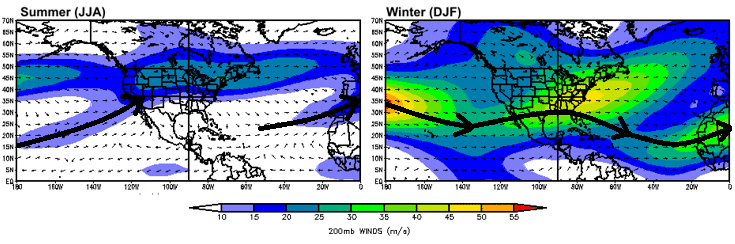
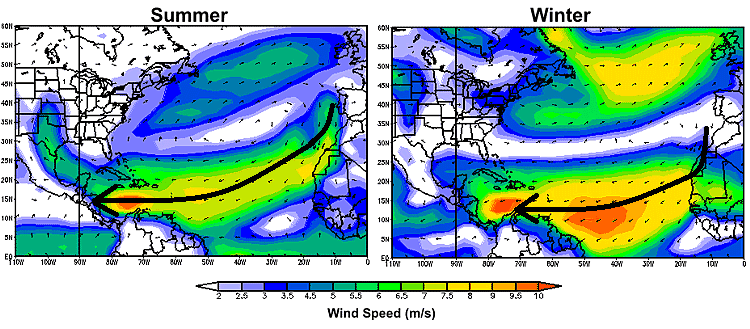
To see the change in the strength of the STJ between summer and winter, compare the average winds near 40,000 feet over North America and adjacent oceans during summer and winter (above). For starters, you can see a signature of fast winds over the central and northern United States. That's the footprint of the mid-latitude jet stream. To mark the STJ, I've used thick black arrows in each image. In summer (left image above), there are two relatively weak streaks of winds associated with the mean position of the summer STJ. One stretches from Hawaii toward the Southwest U.S. and the other heads from the mid-Atlantic Ocean toward northwest Africa. These "streaks" of winds pale in comparison to the robust winter STJ (right image above).
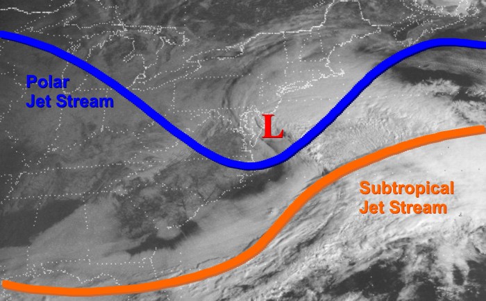
During winter, the robust STJ can contribute to major winter storms over the middle latitudes. The STJ is a semi-permanent feature, and remember that its average location is largely fixed by the rate of rotation of the earth. However, local changes in temperature and pressure gradients can cause parts of the STJ to bulge a bit farther poleward or sag a bit farther southward from time to time. By and large, the northernmost reach of the STJ corresponds to the southernmost extent of the more nomadic mid-latitude jet stream. So, it's safe to assume that the two jet streams sometimes interact, and sometimes the stage can be set for the rapid development of mid-latitude cyclones, particularly over the Atlantic Seaboard, where the natural land-sea temperature contrasts provide favorable breeding grounds.
One such memorable interaction resulted in the surprise Presidents' Day Snow Storm of 1979 [34] for Washington, D.C. and surrounding Middle Atlantic and Southeast states. In this case, the STJ was drawn northward in southwesterly flow ahead of a strong trough in the mid-latitude jet stream (sometimes referred to as the "polar" jet stream, marked in blue). This configuration allowed the STJ to act as a catalyst for the Presidents' Day storm of 1979. Farther to the east, over the Atlantic Ocean, the STJ takes a more eastward and eventual southward turn (off the image to the right) as it starts to return toward its mean position.
In its wake, the Presidents' Day Storm left heavy snow from Georgia to Pennsylvania, as seen on this visible satellite image from 19Z on February 19 [35]. Indeed, many major winter storms in the mid-latitudes benefit from the STJ being drawn northward as in this case. So, while the Hadley Cells regularly control aspects of tropical weather, they can certainly have impacts on weather in the mid-latitudes, too!
In terms of the Hadley Cells [29], we've now covered the ascending branch in the ITCZ, the upper-branch (which culminates in the STJ), and the descending branch that forms the subtropical highs near 30-degrees latitude. Up next, we'll turn our focus to the final branch of the circulation -- the trade winds: the surface flow that returns toward the ITCZ from the subtropics. Read on!
Tricks of the Trades
Prioritize...
Upon completion of this page, you should be able to explain the formation of the trade winds, identify the typical direction from which they blow in each hemisphere, and discuss their role in moisture transport and cloud / precipitation formation.
Read...
Early in this lesson, one of the quirks of tropical weather I mentioned was the tendency for a single surface wind direction to dominate for most of the year. Furthermore, these persistent winds tend to be a bit speedier than we might expect, given the fact that pressure gradients in the tropics are small overall. Now it's time to explore these topics and "close the loop" of the Hadley circulation by talking about the bottom of the circulation -- the trade winds. The near-surface return flow toward the equator from the subtropical highs constitutes the trade winds (you may want to refresh yourself one more time with this Hadley Cell schematic [29]).
Air parcels sinking around the cores of the subtropical highs possess little west-east motion relative to the earth's surface, having lost their residual eastward motion during the long descent from the upper branches of the Hadley Cells. As air on the eastern flanks of the subtropical highs moves equator-ward, it starts turning toward the west, forming the trade winds (as seen in the images of summer and winter wind vectors below). In the Northern Hemisphere, the trade winds blow from the northeast at modest speeds between 10 and 25 miles per hour across the belt of low latitudes, where pressure gradients are typically lax. The trade winds blow from the southeast in the Southern Hemisphere, but we're going to focus most of our analysis on the Northern Hemisphere for simplicity's sake.
How does the northeasterly motion of the trade winds develop and how do they get so "speedy" with such small pressure gradients? The answer to the first question is, of course, the Coriolis force (southward moving air gets directed toward the right, or west, in the Northern Hemisphere). The answer to the second question is a bit more complex and requires us to think really "big picture" about angular momentum for a moment. As parcels move southward toward the equator, their distance from the earth's axis of rotation increases, which would cause them to slow down (like an ice skater stretching out his or her arms in a spin). At first glance, this situation would seem to lead to rather sluggish trade winds, but the trade winds are tricky!
The trade winds are actually a bit speedier than the pressure gradient alone might suggest, and the reason why comes down to conservation of momentum. In an absolute sense (say, to an observer looking down on Earth from space), all air parcels in the atmosphere have some eastward momentum, because the atmosphere moves along with the rotation of the earth (which is toward the east). Even parcels that move westward relative to earth's surface still have eastward momentum overall because the entire atmosphere is moving eastward in an absolute sense. So, when parcels "slow down" as they move equator-ward, what I really mean is that they must lose some of their overall eastward momentum as they move farther away from earth's axis of rotation. As these parcels move southward (in the Northern Hemisphere), they lose some eastward momentum by accelerating in the opposite direction -- toward the west (relative to the earth's surface), as the Coriolis force acts on them.
I'm skipping some of the nitty-gritty details, but the bottom line is that the faster speeds of the trades (compared to what we might think given rather small pressure gradients in the tropics), are a manifestation of the earth and atmosphere trying to conserve angular momentum in an "absolute" sense. Along the way, the trades play a critical role in transporting moisture that feeds the showers and thunderstorms that rise in the ITCZ. As they flow from the subtropics toward the ITCZ, evaporation of ocean water occurs over the vast ocean expanse covered by the trades. To see what I mean, check out the image below. Technically, this image shows something called "latent heat flux," but we can use it as a proxy for evaporation rates (you may recall that "latent heating" refers to the energy exchanges that occur during phase changes).
The trade wind belts display a maximum in "latent heat flux" because of the abundant evaporation that occurs there as the trades flow briskly over open ocean waters. Evaporation increases the amount of water vapor in the lower troposphere as the trades flow toward the ITCZ, and shallow rising currents of moist air frequently yield fields of "trade-wind cumulus clouds" [36] (credit: NASA) throughout the trade-wind belt. Ultimately, however, the additional water vapor gained from evaporation as the trades flow equator-ward helps to feed the tall cumulonimbus clouds that form the showers and thunderstorms of the ITCZ in the ascending branch of the Hadley Cell.
But, along the way, the persistent trades sometimes encounter tall mountains, setting up a scenario with persistent orographic lift (upslope flow). Armed with moisture that evaporated from the oceans, the trades help create some of the wettest places on Earth as air ascends tall mountains. For example, near the summit of Mount Waialeale on the Hawaiian island of Kauai [37], 350 to 400 inches of rain typically fall each year! Much of this rain falls from orographic lift as the persistent trades ascend the windward steep terrain of Mount Waialeale, making the mountain one of the wettest places in the world.
Summary of the Hadley Cell
Now that we've covered the trades, we've completed the entire Hadley circulation. To summarize:
- The ITCZ and the ascending branch develops in response to strong solar heating in the tropics
- In the upper branch, air spirals (thanks to the Coriolis force) poleward toward 30-degrees latitude from the tops of ITCZ thunderstorms, culminating in the subtropical jet stream
- Air converges in the upper troposphere near 30-degrees latitude, causing the formation of the belt of subtropical highs. Air sinks over these latitudes, and warms greatly on descent
- Near the surface, the return flow of air toward the ITCZ forms the trade winds (from the northeast in the Northern Hemisphere; from the southeast in the Southern Hemisphere), which transport moisture (via evaporation of ocean water) to help feed the cumulonimbus clouds of the ITCZ
With our coverage of the Hadley Cell complete, we're going to turn our attention to a couple of weather and climate features of the tropics that you've perhaps heard of, because they can have dramatic impacts on weather even outside the tropics! As it turns out, the trades play an important role in our first topic ("monsoons"). As the ITCZ shifts northward into the Northern Hemisphere during summer, the Southern Hemisphere's southeasterly trades cross the equator and help incite heavy rains in Southeast Asia. Although you've probably heard the term "monsoons" before, as you're about to see, there's much more to them than just rain!
Monsoons: Giant Sea / Land Breezes
Prioritize...
When you've completed this section, you should be able to properly define monsoon and discuss the causes of the Indian and Southeast Asian Monsoons, as well as the resulting weather. You should also be able to compare the size of the wind shifts associated with the Indian Monsoon and the North American Monsoon, as well as define monsoon depressions and discuss the weather associated with them.
Read...
Many tourism guides suggest that the best time to visit Agartala (the capital of the state of Tripura [38] in Northeast India) is October through April. That's largely based on rainfall (and to a lesser extent, temperature). To understand why October through April is the best time to visit Agartala, check out the image below, which documents the rainfall history of Agartala from September 28, 2003, through September 28, 2004. Look at the bar graph of daily rainfall on the lower half of the image. Note that the left vertical axis designates rainfall in inches, while the vertical axis on the right expresses rainfall in millimeters (approximately 25 millimeters equals one inch). Although several inches of rain fell in the first three weeks of October, 2003, the period from October through April was otherwise dry. The running tally of the rainfall on the upper graph (the thick line) is essentially flat during the dry period, holding steady at about 10 inches. But, there was only a slight deficit in rainfall by April (the thin line, which represents the long-term average rainfall, lies above the running tally and the rainfall deficit is shaded in brown), suggesting that such dry conditions are fairly normal.
So, there's no doubt that the period from October through April was dry (and, indeed, it constitutes the "dry season" at Agartala). Then, starting in June, it's as if someone threw a switch and the heavens opened up, with almost 80 inches of rain falling within about six months. Note that, with the exception of a noticeable "break" in early to mid August, it rained most days at Agartala (with a couple of days bringing about nine inches each).
Such definitive dry and rainy seasons are the hallmark of the Indian and Southeast Asian monsoon. Lest you think I've lost all my marbles by lumping the dry period into this discussion of "monsoons", I point out that the word "monsoon" derives from the Arabic word mausim, which translates to "season". Meteorologically speaking, monsoon means "a seasonal wind". Monsoons are actually defined by seasonal shifts in prevailing wind. Yes, it's common to hear people (even some weathercasters) throw out the term "monsoon" for any siege of rainy weather, but such usage is technically incorrect.
Definitive seasonal shifts in wind from Africa to southeast Asia qualify a major portion of the tropical Eastern Hemisphere [39] as the world's major monsoonal region. So, what causes this seasonal shift in wind direction? In a sense, monsoons are much like gigantic sea / land breezes. Recall that the sea breeze develops because of uneven heating between land and water. On a sunny day, the land warms more quickly than adjacent ocean waters, which causes the average density of air columns over land to decrease slightly, which reduces the weight of local air columns and reduces surface pressure. Meanwhile, the air over water remains cooler (and more dense) and an area of high pressure develops offshore. These pressure differences cause low-level air to flow from the water to the land, generating an onshore wind called the sea breeze. At night, the opposite occurs: Land cools off more quickly than adjacent water, and the circulation reverses, resulting in an onshore flow called the land breeze.
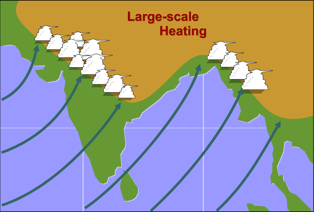
It's no coincidence that the majority of the land in the world's major monsoon region [39] lies north of the equator. Moreover, there's a large expanse of sea that dominates the southern part of the monsoon region, setting the stage for the development of a gigantic sea breeze during the Northern Hemisphere's summer, when intense heating of southern Asia and western North Africa results in a large land-sea temperature gradient. Like its small-scale cousin, a large-scale sea breeze develops and transports moist air inland, paving the way for formidable showers and thunderstorms (check out the schematic on the right). As October ends and the seasonal cooling of the land is well underway, there is a gradual transition to the offshore winds of the winter monsoon (akin to the land breeze at the shore). Indeed, the zone of highest temperature shifts southward, eventually setting up over the Southern Hemisphere.
To examine further, let's focus on India, since it lies near the heart of the major monsoon region. India is hot in the summer, but the temperatures in much of the country actually peak in May. To see how hot India is in May, check out the map long-term average temperatures [40]. The average temperature in parts of India is near 100 degrees Fahrenheit! That's the average of daily high and low temperatures during the month, not just daily highs! The broiling heat of May draws the monsoon trough [41], which is just the regional manifestation of the equatorial trough, northward into India. As this occurs, southeasterly trades in the Southern Hemisphere invade the Northern Hemisphere as convergence with the ITCZ shifts to the Northern Hemisphere. Gradually, these winds turn into southwesterlies over the Arabian Sea and Indian Ocean [42] (in response to the right-deflecting Coriolis force), and moisten as they travel over warm waters. Eventually, the surge of moist southwesterly winds into India fuels the heavy rainfalls during the summer monsoon.
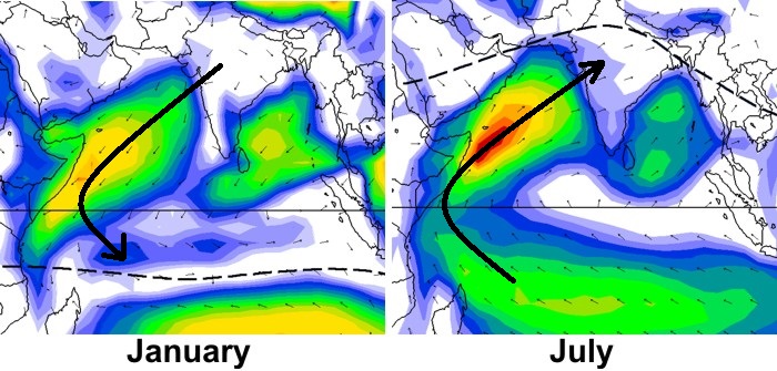
To see how southwesterlies march northward on the south side of the monsoon trough, check out the comparison (below) of surface wind vectors averaged over 30 years during January (left) and July (right). The dashed lines on both images mark the average positions of the monsoon trough. Note that the long-term average position of the monsoon trough in January is south of the equator. In July, however, the trough shifts far to the north.
The bottom line here is that the annual wind reversal over the Indian Ocean and surrounding land areas is the most spectacular seasonal wind shift on this planet. Nowhere else even comes close. India actually experiences a nearly complete reversal in wind direction between meteorological summer and winter [43] (summer average wind vectors on the left; winter on the right). And, it's the large wind shift that defines the monsoon, not rainfall. The rainfall during the summer monsoon is merely an effect of the moist onshore flow, while the dry period in the winter corresponds to the dry offshore flow. But, the shift to dry winds in the winter is just as much a monsoon (the "winter monsoon") as the shift to moist winds and rainy weather in the summer (the "summer monsoon").
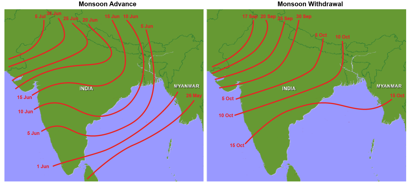
While definitive wind shifts define the monsoon, trends in rainfall help meteorologists keep track of the progress of the monsoon. You see, unlike routine land and sea breezes, which work pretty much like clockwork along the coast, the start and the end of the summer monsoon are not set in stone (the image below shows the average start (left) and end (right) dates). Obviously, definitive shifts in prevailing winds are pieces in the timing puzzle, but sharp increases in consecutive five-day rainfall totals mark the climatological onset date of the summer monsoon (and sharp decreases mark the withdrawal of the summer monsoon). Although the rains of the summer monsoon arrive over Myanmar in May, they do not envelop all of India until well into July. Note the "gradient" of late-May, early-June start dates over southern India. Here, the summer monsoon sometimes advances relatively fast and furious as it sweeps across the southern regions in a spectacular burst. Frequently, however, the onset of the monsoon is not spectacular, tempered by a gradual transition that starts with shifting winds, higher humidity, and subsequent light rains.
Like most things in life, the summer monsoon can be late or early arriving (and late or early leaving). Still these dates give weather forecasters timing guidelines. Regardless of the specifics of the onset of the summer monsoon in any given year, this progression explains why May tends to be the hottest month in India. The onset of the summer monsoon in June brings moist onshore flow, and more numerous showers and thunderstorms begin spreading across the country typically. Moist onshore flow and frequent showers and thunderstorms through the summer months tend to suppress temperatures a bit (it's still hot, but not quite as hot as May).
As mentioned previously, the rain that comes with the summer monsoon isn't constant (breaks in the rain can last a week or two at a time), and a significant portion of the rain that falls during the summer monsoon season is associated with monsoon depressions, which are low-pressure systems that form globally where ever monsoons occur. Monsoon depressions can be responsible for episodes of very heavy rain. For example, from June 10 to June 15, 2004, torrential rains associated with a monsoon depression [44] deluged parts of eastern India. Estimated precipitation from satellite [45] showed rainfall as high as 24 inches during this very wet period. Not surprisingly, such episodes of heavy rain can cause catastrophic flooding.
While the monsoon in India is the most dramatic on Earth, monsoons occur to varying degrees in other parts of the world. Perhaps you've heard weathercasters refer to a "monsoon" in the southwestern United States. By most standards, this North American Monsoon is minor compared to the monsoon in India and the rest of southeast Asia (the wind shift associated with the North American Monsoon is much more subtle). In fact, the wind shift is subtle enough that some scholars don't consider the North American Monsoon to be a "real" monsoon. Regardless, the moist summertime flow is sufficient to fuel slow-moving thunderstorms in the southwestern United States, which can cause serious flash flooding and damage. On August 19, 2003, for example, nearly stationary thunderstorms [46] dumped as much as three inches of rain on Las Vegas, Nevada, in just 90 minutes, causing serious flooding [47]. Unfortunately, flash flooding in Las Vegas is almost a sure bet during the summer monsoon season.
So, while the North American Monsoon pales in comparison to the summer monsoon of India and Southeast Asia, the impacts of the monsoon (details of local wet and dry seasons) are regional in scope. Up next, we'll take a look at a characteristic of tropical weather that has effects which ripple across the entire globe (even beyond the tropics). Read on!
El Niño and La Niña
Prioritize...
Upon completion of this section, you should be able to discuss the changes in ocean temperatures in the equatorial Pacific Ocean associated with El Niño and La Niña, define "anomaly," and connect the development of El Niño and La Niña to changes in the trade winds.
Read...
I suspect that most folks have at least heard of El Niño and perhaps La Niña before. Other than tropical cyclones, they're probably the two tropical weather features that tend to make the news [48] most often because of their impacts on global weather patterns. El Niño, in particular, has been the subject of cartoons and comics [49] and has even been unforgettably spoofed on Saturday Night Live [50].
So, just what exactly are El Niño and La Niña? Well, they're not "tropical storms" (sorry, Saturday Night Live). El Niño is an unusual warming of the waters across the central and eastern equatorial Pacific (approximately from the international date line to the South American coast). La Niña is its cool counterpart. Together, El Niño and La Niña characterize the two phases of the El Niño--Southern Oscillation (ENSO, for short). For the record, the Climate Prediction Center [51] declares the onset of El Niño when the three-month average of sea-surface temperatures in a strip between latitudes five degrees north and south and longitudes 170 degrees West and 120 degrees West [52] exceeds the long-term average by at least 0.5 degrees Celsius. Conversely, the Climate Prediction Center declares a La Niña when the three-month average of sea-surface temperatures is at least 0.5 degrees Celsius below the long-term mean in a similar strip between 150 degrees West and 160 degrees East.
The term, El Niño, as it relates to our discussion, can be traced to the local name that Peruvian fisherman originally gave for the "hesitation" in the normally cold Humboldt ocean current [53] off the west coast of South America that they noticed during December. By "hesitation", I mean the temporary replacement of the Humboldt Current by a weak (and warmer) current flowing southward from equatorial regions. The literal translation of El Niño (from Spanish) is "the boy child", which was a local reference to the Christ child because the "Humboldt hesitation" occurred around Christmastime.
In the context of a "hesitation", El Niño lasted a few to several weeks. Every two to seven years, however, a major breakdown of the Humboldt Current sends large-scale ripples through oceanic and atmospheric patterns over the course of months or even years, which leads to a protracted warming across the central and eastern equatorial Pacific (now known as El Niño). This cycle of warming can be seen in the time series of the sea-surface temperature "anomalies" (in degrees Celsius) in the central Pacific from 1950 through 2017 (below). An anomaly is merely the difference between an observation and the long-term average (anomaly = actual observation - long-term average). Therefore, positive sea-surface temperature anomalies represent warmer-than-normal conditions (marked by orange on the graph), while negative sea-surface temperature anomalies represent cooler-than-normal conditions (marked by blue on the graph). Note that the strongest El Niños occurred in 1982-1983, 1997-1998, and 2015-2016, but a number of other El Niño episodes (the threshold is marked by the faint red line on the graph) have occurred since 1950.
On the other hand, the graph above also shows that a periodic cooling of the waters in the central and eastern equatorial Pacific (La Niña episodes) often occurs in between El Niño episodes. So, what causes this cycle of warming and cooling in the equatorial Pacific? I'm not going to go into great detail about the formation mechanisms of El Niño and La Niña, as they can be complex (and if truth be told, still hold a few mysteries for scientists). But, I do want to give you a basic idea, and to do so, we have to talk a little bit about interactions between the atmosphere and ocean.
When winds blow over the ocean, they exert a "stress" on the surface water, setting it into motion. Given how persistent and reliable the trade winds are, they're very effective at moving ocean water around the tropics. The water doesn't actually move directly with the direction of the wind over time (thanks to the influence of the Coriolis Force), but the end result is that the northeasterly and southeasterly trade winds in the Pacific actually end up pushing water toward the western part of the Pacific basin. As a result, warm water piles up against Indonesia, forming a "mound" of warm water in the western equatorial Pacific. Additionally, this mound of water creates a sloped sea surface. That's right! The surface of the ocean is not flat! You can see this mound of warm water in the western Pacific on this cross-section of ocean temperatures and sea-surface heights from [54]January 1997 (measured from satellites and ocean buoys).
This set up (a mound of warm water toward the western side of the Pacific) is considered the "normal" state of the Pacific Ocean, thanks to the trade winds. But, at irregular intervals every few years, the trade winds become less reliable and weaken. This weakening of the trade winds allows the mound of warm water in the western Pacific to slosh back eastward, warming the surface waters of the central and eastern Pacific, heralding the onset of El Niño. Watch the evolution of this process during the onset of the 1997-1998 El Niño in the animation of ocean temperatures and sea-surface heights from January 1997 through November 1998 below (:46).
Throughout 1997, you can see the mound of warm water slosh eastward as El Niño developed and continued into 1998. But, throughout 1998 the tide turned and the warm water returned to the western Pacific, while the central and eastern Pacific cooled, eventually leading to the La Niña later in 1999 (which actually lasted until 2001).
While a weakening of the trade winds heralds the onset of El Niño, the onset of La Niña is preceded by just the opposite -- a strengthening of the trade winds. When the trade winds strengthen, the mound of warm water in the western equatorial Pacific grows even more than normal, while the central and eastern Pacific become cooler than normal as deep, chilly water surfaces closer to South America.
I've skipped many details here (specifically relating to processes occurring beneath the ocean surface), but I wanted to give you a basic idea of the linkage between weakening trade winds and El Niño, and between strengthening trade winds and La Niña. To help you visualize the development of the unusually warm water in the central and eastern Pacific and see what an El Niño "looks like," check out the animation of global sea-surface temperature anomalies from January 2015 through August 2016 below. Throughout 2015, one of the strongest El Niño episodes on record developed (note pool of above normal sea-surface temperatures near the equator that extends toward the central Pacific from the West Coast of South America).
The 2015-2016 El Niño reached its peak during Northern Hemisphere winter (as is typical), and then during 2016, the El Niño weakened. By July and August, cooler-than-normal waters were evident in the equatorial central and eastern Pacific, signaling the development of La Niña.
Recall that for an El Niño or La Niña episode to be declared, sea-surface temperatures in the central and eastern Pacific need only be 0.5 degrees Celsius above or below normal, respectively (averaged over three months). So, what's the big deal about such seemingly innocuous departures from normal sea-surface temperatures? Well, over the course of several several months (or longer), these warmer or cooler waters modify the overlying atmosphere, and can ultimately have impacts reaching far and wide. What happens in the tropical Pacific does not stay in the tropical Pacific! We'll explore some of the local and global impacts of El Niño and La Niña in the next section.
Local and Global Effects of El Niño and La Niña
Prioritize...
After completing this section, you should be able to discuss the local, regional, and global effects (via teleconnections) of El Niño and La Niña, including changes to the Walker Circulation and patterns of precipitation over the equatorial Pacific, and changes to the subtropical jet stream. However, you need not memorize specific global teleconnections for any particular season or area.
Read...
Even though a seemingly slight warming or cooling of water temperatures in the equatorial Pacific might not seem like a big deal, the impacts of El Niño and La Niña can be dramatic on a global scale. To summarize the impacts of El Niño and La Niña, I'm going to start with local impacts and we'll work our way up through regional impacts and global impacts. In many ways, since El Niño and La Niña are opposites, their impacts are opposite, but that's not always the case!
Local Impacts
I'll start with a direct, local impact of the warmer waters of El Niño. El Niño negatively impacts the living organisms within the marine ecosystem in the eastern equatorial Pacific. Under normal conditions, the nitracline, an underwater boundary that separates cold, deep water with relatively high concentrations of nitrates from shallower water with lower concentrations, lies at a relatively shallow depth. For the record, nitrates serve as nutrients that plants, such as phytoplankton [55] (the base of the ocean's food chain), require for photosynthesis and growth.
With a shallow nitracline, nutrient-rich waters are often brought to the sea surface off the west coast of South America, where they fertilize blooms of phytoplankton that sustain a bounty of fishes. In turn, fish serve as the base of the food chain for seabirds and higher-order mammals that populate the rich and diverse ecosystem in the Galapagos Islands [56]. But, with the onset of El Niño, the nitracline descends deeper below the ocean surface (as warmer-than-normal waters collect near the surface). The end result is that there are notably less nutrients available near the ocean surface, causing a decline in phytoplankton which causes fish to die (or migrate to areas with more nutrients). These negative effects can ripple through the entire food chain in this region of the world. Moreover, El Niño has serious economic impacts on the Peruvian anchovy industry, which eventually translates to higher anchovy prices around the world. But, the impacts of El Niño go beyond sea life (and the price of pizza toppings), because of interactions between the atmosphere and ocean.
Regional Impacts
The "normal" state of the Pacific, with warm water piled up in the western side of the basin near Indonesia impacts vertical motions of air in the atmosphere. The warm waters in the western Pacific Ocean encourage convection over Indonesia (by warming and moistening overlying air, favoring positively buoyant air parcels), while cooler waters in the east-central Pacific tend to suppress convection. As a result, there is a weak but persistent circulation over the equatorial Pacific called the Walker Circulation, which bears the name of Sir Gilbert Walker who, in 1923, was the first to propose this zonal pattern of convection over Indonesia and a tendency for gently sinking air over the eastern equatorial Pacific. The warmth of the overlying air columns in the western Pacific also leads to relatively low density of air columns and lower sea-level pressures in the western Pacific [57] compared to sea-level pressures farther east.
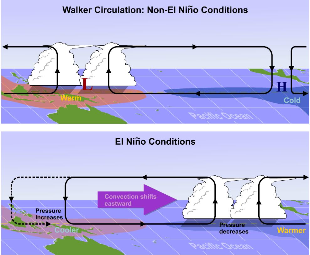
But, since El Niño changes the location of the warm waters in the equatorial Pacific, it alters the Walker Circulation, too. The top schematic above shows the "normal" state of the Walker Circulation, with warm water in the western Pacific causing lower surface pressures there and favoring rising currents of air and convection (showers and thunderstorms). The eastern Pacific, on the other hand, has higher pressures at the surface and is characterized by gently sinking air. In between, the trades transport air toward the western side of the basin near the surface. During an El Niño episode, however, the Walker Circulation is reversed: As water temperatures increase in the eastern and central equatorial Pacific during El Niño, rising air and convection are favored (meaning more showers and thunderstorms than normal). In the western Pacific, where waters aren't as warm as usual (and surface pressures are higher than normal) sinking air is favored (convection is suppressed, meaning fewer showers and thunderstorms than usual).
The changing patterns of showers and thunderstorms associated with the reversed Walker Circulation can bring dramatic consequences. In nations of the western Pacific, a general lack of rain that comes with sinking air can pave the way for drought and wildfires. In the eastern Pacific, typically dry areas can receive a protracted period of recurrent heavy rain during an El Niño, and if the El Niño is strong (sea-surface temperatures as high as three degrees Celsius or more above the long-term average) the onslaught of rain can lead to flash flooding, and widespread destruction.
We can see a prime example of the major changes that El Niño brings by examining the coast of South America from Ecuador southward to northern Chile [58]. This area boasts some of the most extensive coastal deserts on the face of the earth, including the Atacama Desert, which is known as the driest place on Earth. In parts of the Atacama Desert, nary a drop of rain falls for years at a time (check out the bone-dry Atacama Desert from space and on the ground [59]). But, during El Niño, the dryness gives way to showers and thunderstorms that develop in the rising branch of the Walker Circulation, which can drop more rain in one day than normally falls in a decade or more. The heavy rains can result in beautiful desert "blooms," in which the desert floor becomes covered with flowers. The Atacama Desert bloom that occurred during the 2015-2016 El Niño [60] was especially stunning.
So, while the Walker Circulation reverses during an El Niño event, just the opposite happens during La Niña. The Walker Circulation actually becomes stronger than its "normal" state during La Niña. Cooler-than-normal waters in the central and eastern Pacific help to increase sea-level pressures in that region even more, and the sinking air overhead becomes even more pronounced. Meanwhile, stronger trade winds continue to mound warm water in the western Pacific, leading to an even more pronounced signal of rising air and showers and thunderstorms there. In other words, during La Niña, typically wet areas in the equatorial Pacific tend to get a bit wetter, and typically dry areas tend to be even drier.
Global Impacts
But, what happens in the tropical Pacific doesn't stay in the tropical Pacific! The impacts of El Niño and La Niña ripple out across the globe largely by way of their impacts on the subtropical jet stream (STJ), which increase the probability that it reconfigures into persistent and distinctive patterns, particularly during the cold season. In turn, this reconfiguration produces ripples that alter weather patterns, called teleconnections. In a nutshell, a teleconnection is a correlation between a persistent weather pattern occurring in one region (in the case of El Niño or La Niña, the eastern and central equatorial Pacific) with recurrent weather patterns in other regions of the world.
So, how can El Niño or La Niña impact the STJ? I'll focus on El Niño for simplicity. As it turns out, over the course of several months, the warm waters of El Niño modify the overlying air columns, making them a bit warmer than normal, too. For example, check out the temperature anomalies near the top of the troposphere from January to March 1998 [61] (during a strong El Niño). It's pretty clear that the warmth of El Niño had been transferred all the way to the upper troposphere, with a large area of warmer than normal air in the central and eastern tropical Pacific. These alterations to the temperature patterns aloft also impact the pressure gradients aloft, causing the STJ to strengthen during an El Niño. To see what I mean, compare the long-term average of winds near the top of the troposphere during January - March to those during January - March, 1998 (above). There's no doubt that during the strong El Niño of 1997-1998, the STJ was more robust than normal. Its fastest winds extended farther across the Pacific and it was stronger near the southern United States, too.
Changes to the STJ over months can lead to recurrent weather patterns that cause areas of extreme weather across the globe. For example, in winter, a stronger STJ can play a more active role in the development of mid-latitude cyclones, which can cause recurrent storminess in California and along the southern tier of the United States (and sometimes up the East Coast, too). Frequent visits from strong mid-latitude cyclones can also lead to more active tornado outbreaks along the Gulf States and Florida during El Niño winters. But, there are many more teleconnections! To see what I mean, check out these graphics showing typical large-scale temperature and precipitation anomalies [62] that accompany El Niño and La Niña during Northern Hemisphere winter and summer. In North America, during winter, perhaps the most striking effect of El Niño is a large warmer-than-normal area from Alaska stretching across western and central Canada into the northern tier of the United States. The southern United States, on the other hand, tends to be cooler-than-normal (especially the Gulf States) and wet, which fits with the active parade of mid-latitude cyclones that can trek across the southern U.S. during El Niño winters.
Also note that in some areas, the effects of La Niña tend to be largely the opposite of the effects of El Niño, which makes sense because La Niña is the opposite of El Niño. But, in some areas of the world (more commonly in Northern Hemisphere summer, when El Niño and La Niña tend to be weaker), their impacts bear no resemblance to each other at all. So, La Niña's teleconnections aren't always as simple as assuming the opposite of whatever happens in a particular area during an El Niño. The atmosphere is more complex than that!
Still, knowing the state of the tropical Pacific can help weather forecasters with long-range weather outlooks [64] (say, for a month, or a particular season) in other parts of the world. But, even knowing that an El Niño or La Niña is present offers few complete guarantees. To understand why, allow me to use an analogy. Have you ever thrown rocks into a pond and watched the waves that each rock's splashdown creates? Bigger rocks make bigger waves, and if you throw multiple rocks, interesting things happen when ripples from different rocks encounter each other. If you throw enough rocks into the pond, eventually it's virtually impossible to attribute the waves reaching the bank of the pond to any single rock because the interactions are too complex.
And so it is with the atmosphere. Indeed, a barrage of "rocks" thrown into the pond of air we call the atmosphere determine weather patterns across the middle latitudes, including the distribution of continents and oceans, mountains, the extent of ice and snow cover, and, yes, El Niño and La Niña. So, please understand that no single storm can be blamed on El Niño or La Niña. Such an assignment of blame is tantamount to attributing a ripple of water reaching the side of a stone-infested pond to a single rock. Could El Niño or La Niña play an important role? Of course, with the stipulation that strong El Niños and La Niñas play more pivotal roles in fashioning hemispheric and global patterns of weather (metaphorically, strong El Niños and La Niñas are bigger rocks that make bigger splashes that produce bigger ripples). But, El Niño or La Niña does not single-handedly take over the atmosphere and dictate a snowstorm here, a drought there, and so on and so forth. They merely make certain weather patterns more (or less) likely than usual over the course of months or seasons.
Furthermore, no two El Niños or La Niñas are exactly alike, so any single El Niño or La Niña may not produce temperature and precipitation patterns exactly like the idealized graphics I showed you (the Gulf States aren't always cool and wet in the winter during an El Niño, for example). The strength of the El Niño or La Niña matters, as does the specific location of the largest sea-surface temperature anomalies in the tropical Pacific. Furthermore, El Niño or La Niña is just one "rock" being thrown into the atmospheric pond. While forecasters can use knowledge of El Niño or La Niña teleconnections to help them make long-range outlooks for a given month or season, other atmospheric features can mask the influence of El Niño or La Niña entirely. In other words, sometimes there are bigger rocks making bigger splashes in the atmospheric pond, which makes long-range forecasts very challenging! But, make no mistake about it, whenever you see a long-range weather outlook, most likely the forecasters who prepared it incorporated the state of the tropical Pacific into their forecast rationale. So, El Niño and La Niña are certainly important factors on a global scale! They can even affect tropical cyclone activity, which is one topic we haven't explored in this lesson. That's because tropical cyclones deserve their own lesson (up next)!