Overview

In previous lessons, we were able to explain physical and chemical processes using only algebra and differential and integral calculus. Thermodynamics, moist processes, cloud physics, atmospheric composition, and atmospheric radiation and its applications can all be quantified (at this level of detail) with fairly simple mathematics. However, more math skill is required to understand and quantify the dynamics of the atmosphere.

This lesson introduces you to the math and mathematical concepts that will be required to understand and quantify atmospheric kinematics, which is the description of atmospheric motion; and atmospheric dynamics, which is an accounting of the forces causing the atmospheric motions that lead to weather. Weather is really just the wind (the motion of air in the horizontal and the vertical) and the consequences of the wind. Wind, which has both direction and speed, is best described using vectors.

The Earth is a spinning, slightly squashed sphere. The atmosphere is a tenuous thin layer on this orb, so from a human’s limited view, the Earth appears to be flat. For some applications, a simple Cartesian coordinate system, with three dimensions in the x, y, and z directions, seems like a good way to mathematically describe motion. For processes that occur on the larger scale, where the Earth’s curvature is noticeable, we must resort to using coordinates that are natural for a sphere.

The way wind direction is described sprang out of wind observations, and is now firmly implanted in the psyche of every weather enthusiast: easterly, northerly, westerly, and southerly. This wind convention, however, is quite different than that used in the equations that govern atmospheric motion, which are the basis of weather forecast models. Here we will see that a conversion between the two conventions is straightforward but requires some care.

Finally, we will see that movement of air can either be described by an observer at a fixed location (called the Eulerian framework) or by someone riding along with a moving parcel of air (called the Lagrangian framework). These two points-of-view are very different, but we will see that they are related to each other by advection, which is just the movement of air with different properties (such as temperature, pressure, and humidity) from a place upwind.

With this math and these concepts you will be ready to take on atmospheric kinematics and dynamics.

Learning Objectives

By the end of this lesson, you should be able to:

• calculate partial derivatives
• implement vector notation, the dot product, the cross product, and the del operator
• explain the different coordinate systems and how they are used
• convert between math and meteorological wind directions
• calculate temperature advection at any point on a map of isotherms (lines of constant temperature) and wind vectors

Questions?

If you have any questions, please post them to the Course Questions discussion forum. I will check that discussion forum daily to respond. While you are there, feel free to post your own responses if you, too, are able to help out a classmate.

8.1 This is why partial derivatives are so easy...

In your first calculus class you learned about derivatives. Suppose we have a function f that is a function of x, which we can write as f(x). How does f change with a very small change in x? This change is quantified by the derivative of f with respect to x.

What about a new function that depends on two variables, h(x,y)? This function could, for example, give the height h of mountainous terrain for each horizontal point (x,y). So what is the derivative of h with respect to x? One way we determine this derivative is to fix the value of y = y₁, which is the same as assuming that y is a constant and then taking the ordinary derivative of h with respect to x. Suppose we take a slice through the mountain in the x-direction at a fixed value of y = y₁, that is, y kept constant. How does h vary with a small change in x on this slice? This change is quantified as 

This is called the partial derivative of h with respect to x. It’s pretty easy to determine because we do not need to worry about how y might depend on x. 

Similarly, we can find the partial derivative of h with respect to y. In this case, we assume that x is constant and then take the ordinary derivative of h with respect to y. This change is quantified as 

Are the partial derivatives of h with respect to x and to y the same? Try different functions for h(x,y) to see if you can find one for which they are equal for all values of x and y. (hint: Try h(x,y) = a constant.) Can you find any others?

8.2 What you don’t know about vectors may surprise you!

Remember that a scalar has only a magnitude while a vector has both a magnitude and a direction. The following video (12:33) makes this difference clear.

Typically the vectors used in meteorology and atmospheric science have two or three dimensions. Let’s think of two three-dimensional vectors of some variable (e.g., wind, force, momentum):

Sometimes we designate vectors with bold lettering, especially if the word processor does not allow for arrows in the text. When Equations [8.3] are written with vectors in bold, they are:

Yet another notation uses parentheses and commas, as in A = (A_x, A_y, A_z). Be comfortable with all of these notations.

In the equations for vectors, A_x and B_x are the magnitudes of the two vectors in the x (east–west) direction, for which $\stackrel{\rightharpoonup }{i}$or i is the unit vector; A_y and B_y are the magnitudes of the two vectors in the y (north–south) direction, for which $\stackrel{\rightharpoonup }{j}$ or j is the unit vector; and A_z and B_z are the magnitudes of the two vectors in the z (up–down) direction, for which $\stackrel{\rightharpoonup }{k}$ or k is the unit vector. Unit vectors are sometimes called direction vectors.

Sometimes we want to know the magnitude (length) of a vector. For example, we may want to know the wind speed but not the wind direction. The magnitude of $\stackrel{\rightharpoonup }{A}$ , or A, is given by:

We often need to know how two vectors relate to each other in atmospheric kinematics and dynamics. The two most common vector operations that allow us to find relationships between vectors are the dot product (also called the scalar product or inner product) and the cross product (also called the vector product).

The dot product of two vectors A and B that have an angle $\beta$ between them is given by:

The dot product is simply the magnitude of one of the vectors, for example A, multiplied by the projection of the other vector, B, onto A, which is just $Bcos\beta$. Thus, if A and B are parallel to each other, then their dot product is AB. If they are perpendicular to each other, then their dot product is 0. The dot product is a scalar and therefore has magnitude but no direction.

Also note that the unit vectors have the following properties:

Note that the dot product of the unit vector with a vector simply selects the magnitude of the vector's component in that direction ($\overrightarrow{i}·\overrightarrow{A}=A_x$) and that the dot product is commutative $(\overrightarrow{A}·\overrightarrow{B}=\overrightarrow{B}·\overrightarrow{A})$ .

Equation [8.4] can be rearranged to yield an expression for $\cos \beta$ in terms of the vector components and vector magnitudes:

The cross product of two vectors A and B that have an angle $\beta$ between them is given by:

The magnitude of the cross product is given by:

where $\beta$ is the angle between A and B, with $\beta$ increasing from A to B.

Note that the cross product is a vector. The direction of the cross product is at right angles to A and B, in the right hand sense. That is, use the right-hand rule (have your hand open, curl it from A to B, and A x B will be in the direction of your right thumb). The magnitude of the cross product can be visualized as the area of the parallelogram formed from the two vectors. The direction is perpendicular to the plane formed by vectors A and B. Thus, if A and B are parallel to each other, the magnitude of their cross product is 0. If A and B are perpendicular to each other, the magnitude of their cross product is AB.

The following video (2:06) reminds you about the right-hand rule for cross products.

It follows that the cross products of the unit vectors are given by:

Note finally that $\overrightarrow{A}\times \overrightarrow{B}=-\overrightarrow{B}\times \overrightarrow{A}$.

We sometimes need to take derivatives of vectors in all directions. For that we can use a special vector derivative called the Del operator, $\overrightarrow{\nabla }$.

Del is a vector differential operator that tells us the change in a variable in all three directions. Suppose that we set out temperature sensors on a mountain so that we get the temperature, T, as a function of x, y, and z. Then $\overrightarrow{\nabla }$T would give us the change of T in the x, y, and z directions.

The Del operator can be used like a vector in dot products and cross products but not in sums and differences. It does not commute with vectors and must be the partial derivative of some variable, either a scalar or a vector. For example, we can have the following with Del operator and a vector A:

8.3 Describing weather requires coordinate systems.

In meteorology and other atmospheric sciences, we mostly use the standard x, y, and z coordinate system, called the local Cartesian coordinate system, and the spherical coordinate system. Let’s review some of the main points of these two systems.

Local Cartesian Coordinate System

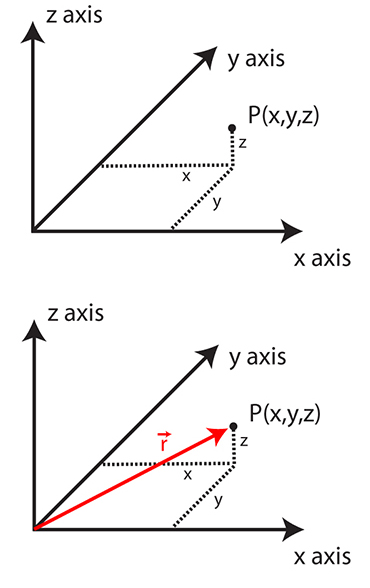
The local Cartesian coordinate system applies to three dimensions (as seen in the figure below). The convention is simple:

• The zero point, x = y = z = 0 or (0,0,0), is arbitrary.
• x increases to the east; x decreases to the west.
• y increases to the north; y decreases to the south.
• z increases going up; z decreases going down.
• A distance vector extending from the origin to (x,y,z) is given by r = i x + j y + k z.

Unit vectors (length 1 along standard coordinates) are i (east); j (north); k (up).

Often we will consider motion in two dimensions as being separate from motions in the vertical. We usually denote the horizontal with a subscript H; for example, r_H = i x + j y, where r_H is a horizontal distance vector.

This coordinate system works well over relatively small scales on Earth, perhaps the size of an individual state, where Earth's curvature is not important. This is why the qualifier "local" is used in the name of the coordinate system. This coordinate system does not work so well for large-scale motion on Earth, which is spherical.

Local Cartesian coordinate system.

Credit: W. Brune

The local Cartesian coordinate system when placed on the globe.

Credit: W. Brune

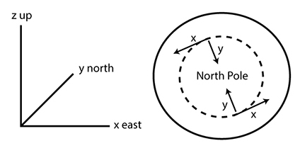
When we place the Cartesian coordinate system on a sphere, note that x always points toward the east, y always points toward the north, and z always points up along the direction of Earth’s radius (as seen in the figure above).

Spherical Coordinate System

Life would be much easier if the Earth were flat. We could then use the local Cartesian coordinate system with no worries. But the Earth is very nearly a perfect sphere, which implies that to accurately describe motion, we must take the Earth’s spherical shape into account.

Spherical coordinate system.

Credit: Artima Developer [4]

We use the following terms:

• r = distance from the center of the Earth
• $\Phi$ = latitude (–90^o to +90^o, or –$\pi$ /2 to +$\pi$/2)
• $\lambda$ = longitude (–180^o to 180^o, or –$\pi$ to +$\pi$)
• State College, PA is at $\Phi ={40.8}^o and\lambda =-{77.9}^o$ .

Note that 1^o of latitude is always 111 km or 60 nautical miles, but 1^o of longitude is 111 km only at the equator. It is smaller in general and equal to 111 km x cos($\Phi$). Note that 1 nautical mile = 1.15 miles.

To find the horizontal distance between any two points on Earth's surface, we first need to find the angle of the arc between them and then we can multiply this angle by Earth's radius to get the distance. To find the angle of the arc, $\Delta \sigma$ , we can use the Spherical Law of Cosines:

where the latitude and longitude of the two points are ${\Phi }_1,{\lambda }_1 and{\Phi }_2,{\lambda }_2$ , respectively and $\Delta \lambda =|{\lambda }_1-{\lambda }_2|$ is the absolute difference between the longitudes of the two points. Note that the angle of the arc must be in radians, where $2\pi radians={360}^o$. To find the distance, simply multiply this arc angle by the radius of the Earth, 6371 km.

In summary, we will use a local Cartesian coordinate system when our scales of interest are not too large (synoptic scale or smaller), but will need to use spherical coordinates when the scale of interest is larger than synoptic scale.

For another explanation of these two systems, visit this Coordinate Systems website [5].

Vertical Coordinates

Three different vertical coordinates are used in meteorology and atmospheric science: height, pressure, and potential temperature.

We have already introduced the vertical coordinate z, which is a height, usually in m or km, above the Earth's surface in the local Cartesian coordinate system; z is related to r in spherical coordinates through r = a + z, where a is the Earth's radius. The vertical coordinate z is the most commonly used in meteorology and in any process that involves getting off the ground, such as flight. Often pilots talk about flight levels, which are measured in hundreds of feet. So, flight level 330 is about 10 km altitude.

Another useful vertical coordinate is pressure, which decreases with height. Pressure is often a useful vertical coordinate in dynamics calculations. To a good approximation, pressure falls off exponentially with height, p = p_oexp(-z/H), as we learned in Lesson 2, so that ln(p) is fairly linear with height. We’ll get into this in greater detail later. For now, consider the following table of typically used pressure heights:

A third important vertical coordinate is potential temperature, $\theta$ (Equation 2.58). This quantity is the temperature that an air parcel would have if it were brought to a pressure of 1000 hPa without any exchange of heat with its surroundings. This vertical coordinate has a nice property: air parcels tend to move on surfaces of constant potential temperature because moving on such a surface requires no energy. This coordinate is particularly useful in the stratosphere, where the rapid increase with altitude tends to keep air motion stratified.

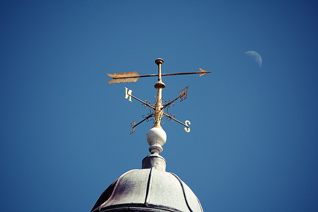
8.4 Do you need a weathervane to see which way the wind blows?

Weathervane

Credit: Justin Otto [6] via flickr

Meteorologists use terms such as northeasterlies and southerlies when they describe winds. These terms designate directions that the winds come from. But when we think about the dynamic processes that cause the wind, we use the conventions for direction that are common in mathematics and in coordinate systems like the Cartesian coordinate system. The conversion between the two conventions—math and meteorology—is not simple. However, we will show you a simple way to do the conversion (see the second figure below).

Math Wind Convention

The wind vector is given by U = i u + j v + k w. The wind vector points to the direction the wind is going.

The subscript “H” will be used to denote horizontal vectors, such as the horizontal velocity, U_H = i u + j v  (though note that sometimes the symbols V , v_H, and v will be used to denote the horizontal velocity). The magnitude of U_H is U_H = (u² + v²)^1/2. The math wind angle, $\alpha$, is the angle of the wind relative to the x-axis, so that tan($\alpha$) = v/u and the angle increases counterclockwise as the direction moves from the eastward x-axis ($\alpha$ = 0^o) to the northward y-axis ($\alpha$ = 90^o) .

Meteorology Wind Convention

In this station weather plot, the wind is blowing from the southwest.

Credit: NOAA National Weather Service

The meteorology wind convention is often used in meteorology, including station weather plots [7]. The wind vector points to the direction the wind is coming from. The angle is denoted by delta, $\delta$, which has the following directions:

Relationship Between Math and Meteorology Wind Conventions

Meteorology angles, designated by $\delta$, increase clockwise from the north (y) axis. Math angles, designated by $\alpha$ , increase counterclockwise from the east (x) axis.

Diagram for converting between meteorology and math wind directions for winds blowing from three different directions. Note that the part of the wind line that has the barbs points toward the direction the wind is blowing from. In this diagram, we have extended the line past the center of the axis to indicate the direction that the wind is blowing to because this is the line needed for the math angle.

Credit: W. Brune

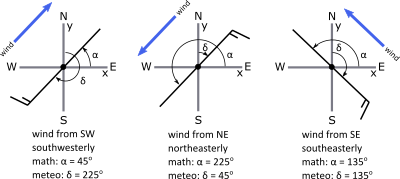
In the diagram on the left, the wind is southwesterly, the meteorology angle (measured clockwise from the north or y-axis) δ = 225^o , and the math angle (measured counterclockwise from the east or x-axis) $\alpha ={45}^o$. If the wind is northerly (southward), the wind vane points to the north, the wind blows to the south, δ = 0^o and α = 270^o. If the wind is westerly (eastward), δ = 270^o and α = 0^o.

Note that in all cases, we can describe the relationship between the math and the meteorology angles as:

$$mathangle=270^{o }-meteorologyangle$$

When the meteorology angle is greater than 270^o, the math angle will be negative but correct. However, to make the math angle positive, simply add 360^o.

Drawing a figure like those shown in the figure above often helps when you are trying to do the conversion. The following video (2:17) explains the conversion between meteorology and math wind angles using the figure above.

8.5 Gradients: How to Find Them

The gradient of a variable quantifies the magnitude and direction of the maximum change of the variable as a function of distance in space. For instance, the temperature gradient gives the maximum amount of temperature change in space and the direction of that maximum temperature change. Thus, a gradient is a vector.

We can find the gradient in Cartesian coordinates by using the del operator, which is also called the nabla or gradient operator,  which is a vector that finds the partial derivative of a variable (please review 8.1) in each direction.

$$ \vec{\nabla}_{H}=\vec{i} \frac{\partial}{\partial x}+\vec{j} \frac{\partial}{\partial y}+\vec{k} \frac{\partial}{\partial z} $$

[8.10]

$$ \vec{\nabla}_{H}=\vec{i} \frac{\partial}{\partial x}+\vec{j} \frac{\partial}{\partial y} $$

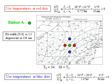
To see how we can calculate gradients, lets start with the commonly used gradient: the horizontal temperature gradient. Look at the surface temperature map for the United States on 8 September 2012.

Surface temperature map for North America on 8 September 2012. Temperatures are in ^oF. For a point in western Kentucky, you can see that the maximum change in temperature with distance is the the southeast. Can you find a location for which the maximum change is to the southwest? How about for the maximum change to the east? 

Credit: Unisys

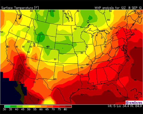
With the temperature data that was used to generate the map above, a computer can easily calculate the gradients for every location. However, you can get a better understanding of gradients by using a map, ruler, and the following mathemantical equations to estimate gradients. First, we show you how to find distances on a map using a ruler. Watch this video (2:12) on finding distances:

Example of a gradient and the math required to calculate the gradient magnitude and direction.

Credit: H.N. Shirer

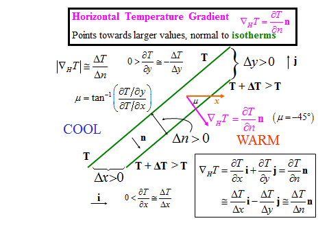
We can calculate a gradient for every point on the map, but to do this we need to know the change in the temperature over a distance that is centered on our chosen point. One approach is to calculate the gradients in the x and y directions independently and then determine the magnitude by:

and the direction by:

The partial derivatives are approximately equal to changes over small distances. Let's assume that the temperature gradient is approximately constant around a location. Then, integrating the equation 8.11, which is the definition of a horizontal gradient, yields

$$ \Delta T = \nabla_{H} T \cdot \Delta n = (\partial T / \partial x) \Delta x + (\partial T / \partial y) \Delta y.$$

[8.14]

For constant y, ∂T/∂x=ΔT/Δx. For constant x, ∂/T/∂y=ΔT/Δy. Thus we can replace partial derivatives with finite changes that we can measure in temperature and distance.

We can program a computer to do these calculations. However, often we just want to estimate the gradient. The gradient can be determined by looking at the contours on either side of the point and computing the change in temperature over the distance. These partial derivatives can be approximated by small finite changes in temperatures and distances, so that $\partial$ is replaced by $\Delta$ in all places in these equations. We can calculate gradients by using “centered differences” as shown in the figures below.

Calculating the temperature gradient in the x (top) and y (bottom) directions using the centered difference method.

Credit: H.N. Shirer

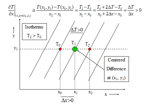
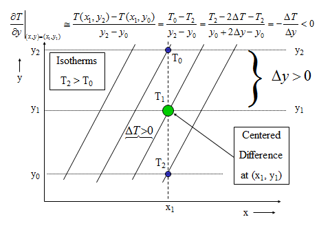
We then calculate the magnitude with Equation [8.12] and the direction with Equation [8.13], where we replace the partial derivatives with the small finite differences in all places in these equations.

Example of an estimation of the gradients in the x and y directions. To get an idea of the horizontal scale, you can estimate distances using the known size of a state or country, in this case, Pennsylvania, which is on average 470 km (254 nm, nautical miles, 290 miles) in the x (east–west) direction and 250 km (135 nm, 155 miles) in the y (north–south) direction for the parts where the north and south borders are parallel lines.

Credit: H.N. Shirer

The magnitude and direction are:

$$\begin{array}{l}\left|{\nabla }_{H}T\right|=\sqrt{{\left(\frac{\Delta T}{\Delta x}\right)}^2+{\left(\frac{\Delta T}{\Delta y}\right)}^2}= \sqrt{{\left(\frac{4{}_{}{}^{\text{o}}\text{F}}{45\text{ nm}}\right)}^2+{\left(\frac{-4{}_{}{}^{\text{o}}\text{F}}{84\text{ nm}}\right)}^2}=0.1{}_{}{}^{\text{o}}\text{F}\text{/nm}\hfill \\ \mu = {\tan }^{-1}\left(\frac{\raisebox{1ex}{$\Delta T$}\!\left/ \!\raisebox{-1ex}{$\Delta y$}\right.}{\raisebox{1ex}{$\Delta T$}\!\left/ \!\raisebox{-1ex}{$\Delta x$}\right.}\right)={\tan }^{-1}\left(\frac{\raisebox{1ex}{$-4$}\!\left/ \!\raisebox{-1ex}{$84$}\right.}{\raisebox{1ex}{$4$}\!\left/ \!\raisebox{-1ex}{$45$}\right.}\right)=-{28}^{\text{o}}\text{, which points to the southeast}\hfill \end{array}$$

When you calculate the arctangent, keep in mind that the tangent function has the same values every 180^o or every π radians. If you get an answer for the arctangent that is 45^o, how do you know whether the angle is really 45^o or 45^o + 180^o = 225^o? The gradient vector always points towards higher values, so always choose the angle so that the gradient vector points toward the warmer air. Alternatively, if ∂T/∂x is greater than 0, choose the value of the arctangent between –90^o and 90^o, whereas if ∂T/∂x is less than 0, add 180^o.

Recap of the process for calculating the temperature gradient:

1. Determine the distance scale by any means that you can. Sometimes it is given to you; sometimes you can scale off a ruler; sometimes you just estimate it using the size of known boundaries.
2. Determine the spacing between the isotherms.
3. Find the temperature change in the x and y directions using the centered difference method. These two numbers, $\Delta T/\Delta xand\Delta T/\Delta y$, are needed to calculate both the gradient magnitude and the gradient direction. Note that $\Delta T/\Delta xand\Delta T/\Delta y$ can be either positive or negative.
4. Calculate the magnitude by finding the square root of the squares of the gradients in the x and y directions (i.e., $\Delta T/\Delta xand\Delta T/\Delta y$).
5. Calculate the direction of the gradient vector by finding the arctangent of the y-gradient divided by the x-gradient. Pay attention to the direction—make sure that it points toward the warmer air.

Now watch this video (3:52) on finding gradients:

Finding Gradients

Click here for transcript of the Finding Gradients video.

We can calculate the gradient by using the method that's described in the lesson. Let's pick a point in Pennsylvania about here, and then we'll calculate the gradient for that point. We will first look at the gradient in the x direction which goes along, and it's parallel with the North and South boundaries of Pennsylvania. We'll use the method of center differences that's described. We'll look at this contour here, this isotherm, and this one over here on the other side. And we note that this distance here is very, very similar to the distance of Pennsylvania between the parallel borders, which is 135 nautical miles. And so each one of these contours is four degrees Fahrenheit. So we have two of them, so 8 divided by 135 nautical miles gives us a gradient in the x direction of 0.059 degrees Fahrenheit per nautical miles. Now we can do the y direction, so we pick two points here. One here and one about here to be on the gradients. And we note that this is a little bit more than half the height of Pennsylvania. It's actually about 80 nautical miles. But also note that as y goes more positive, the temperature becomes more negative and therefore, we have to use minus 8 over 80. And we get, for the gradient in the y direction, minus 0.1 degrees Fahrenheit per nautical miles. When we put these in to get the magnitude-- it's the square root of the squares-- we see that we end up with 0.12 degrees Fahrenheit per nautical mile with a magnitude of the gradient. To find the direction of the gradient we see that mu, the angle with respect to the x-axis-- so this is a math angle. It's equal to the arctangent of the gradient in y divided by the gradient in x. And so that would be the arctangent of minus 0.1 over 0.059, which is minus 59 degrees. And that is, of course, measured from the x-axis here. So that is measured from this direction here like this, and so that's minus 59. And it's the same as if we went all the way around and we would get 301 for alpha if we were looking at the math angle. Now, we can look and get an idea about gradients and other places really quickly, so let's just take this point in Central Oregon. So now x is going like this over here, and so we see that the gradient in the East West direction, or x direction is-- to go to another country you have to go very, very far, and so that would be 8 degrees. It's so far the really the gradient is essentially 0. Whereas if we go in the North South direction-- that is in the y direction here-- we see that there's quite a substantial distance here. And so, since this is 8 degrees, just like this is 8 degrees over here, then what that means is the gradient is going to be quite a bit smaller in this direction than it is in Pennsylvania here where the isotherms are much, much closer together. So we would expect a gradient that's a fourth or a fifth of the gradient that we got for Pennsylvania, and so it'll be very weak. Nonetheless, it'll point toward the hotter air, and it'll look something like this.

A word about finding gradients in the real world. Sometimes the centered differences method is difficult to apply because the gradient is too much east–west or north–south. For instance, in the temperature map at the beginning of this section, the x-gradient is hard to determine by the centered difference method in the Oklahoma panhandle and the y-gradient is hard to determine in central Pennsylvania because in both cases, the temperature hardly changes in those directions. In these cases, you could say that the gradient in that direction equals 0, but then your computer program might have a hard time finding the arctangent. One way around this problem is to put in a very small number for the gradient in that direction, say 1 millionth of your typical gradient numbers, to do the calculation.

A second word about finding gradients in the real world. When you are finding temperature gradients from a temperature map, it is sometimes hard to determine the temperature gradient at some locations because the isotherms are not evenly spaced and can be curvy. Don't despair! Use your best judgment as to what the gradients are. Check your answers for the magnitude and direction of the temperature gradient vector by estimating the magnitude and direction by eyeballing the normal to the isotherms at that location and pointing the gradient vector to the warmer air. If your calculated direction is very different from your eyeballed value by more than, say, 45^o, check your math.

Quiz 8-3: Grading your gradients.

1. Find Practice Quiz 8-3. You may complete this practice quiz as many times as you want. It is not graded, but it allows you to check your level of preparedness before taking the graded quiz.
2. When you feel you are ready, take Quiz 8-3. You will be allowed to take this quiz only once. Good luck!

8.6 What You Experience Depends on Your Point of View: Eulerian vs. Lagrangian

A car travels at the same speed and direction as a thunderstorm

Credit: Nicholas A.Tonelli [8] via flickr

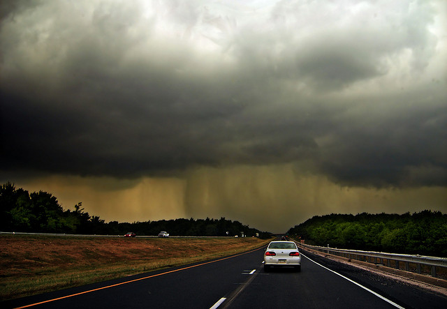
Suppose you were driving underneath an eastward-moving thunderstorm at the same speed and in the same direction as the storm, so that you stayed under it for a few hours. From your point-of-view, it was raining the entire time you were driving. But from the point-of-view of people in the houses you passed, the thunderstorm approached, it rained really hard for twenty minutes, and then stopped raining.

If the people in houses formed a network of observers, and if they talked to each other, they would find that the thunderstorm moved rapidly from west to east in a path that rained on some houses and missed others. This point-of-view is called the Eulerian description because observers are at fixed locations and see the storm only when it is over them. You, on the other hand, followed along with the thunderstorm; any changes you saw were due to changes in the thunderstorm’s intensity only. Your point-of-view was a Lagrangian description because you stayed with the storm.

We can now generalize these ideas to any parcel of air, not just a thunderstorm. An air parcel is a blob of air that hangs more-or-less together as it moves through the atmosphere, meaning that its mass and composition are conserved (i.e., not changing) as it moves. It has a fairly uniform composition, temperature, and pressure, and has a defined velocity. An air parcel needs be large enough so that thermodynamic properties such as temperature, pressure and dewpoint temperature are well defined, but small enough so that it responds quickly to thermodynamic changes induced by air motions.  Air parcel change shape as they move in air and bump into other air parcels. Even though air parcels do not live forever, they are very useful concepts in explaining the differences between the Eulerian and Lagrangian frameworks.

To Summarize

Here's an interesting fact. Radiosonde measurements are considered Eulerian for continental or global networks that span thousands of kilometers because they measure properties like temperature and humidity at most a few 10's of kilometers from their launch site. However, radiosonde measurements are actually neither Eulerian nor Lagrangian because a radiosonde moves in air but does not follow the same air parcel. A cup anemometer or sonic anemometer mounted on a stationary tower is an example of a Eulerian method of measuring wind velocity.

8.7 Can the Eulerian and Lagrangian frameworks be connected?

Changes over time in properties, such as temperature and precipitation, can be expressed in Lagrangian and Eulerian frameworks, and often the changes are different in the two frameworks (as in the precipitation change for the thunderstorm example). We can express these changes mathematically with time derivatives. Suppose we have a scalar, R, which could be anything, but let’s make it the rainfall rate. It is a function of space and time:

To find the change in the rainfall rate R in an air parcel over space and time, we can take its differential, which is an infinitesimally small change in R:

where dt is an infinitesimally small change in time and dx, dy, and dz are infinitesimally small changes in x, y, and z coordinates, respectively, of the parcel.

If we divide Equation [8.15] by dt, this equation becomes:

where dx/dt, dy/dt, and dz/dt describe the velocity of the air parcel in the x, y, and z directions, respectively.

Let’s consider two possibilities:

Case 1: The air parcel is not moving. Then the change in x, y and z are all zero and:

So, the change in the rainfall rate depends only on time. $\frac{\partial R}{\partial t}$ is called the Eulerian or local time derivative, also called the local derivative. It is the time derivative that each of our weather observing stations record.

Case 2: The air parcel is moving. Then the changes in its position occur over time, and it moves with a velocity, $\overrightarrow{U}=\overrightarrow{i}u+\overrightarrow{j}v+\overrightarrow{k}w$ , where:

A special symbol is given for the derivative when you follow the air parcel around. It is called the substantial derivative, also called the Lagrangian derivative, material derivative, or total derivative and is denoted by:

Mathematically, we can express this equation in a more general way by thinking about the dot product of a vector with the gradient of a scalar as we did in an example of the del operator:

where the second term on the right hand side is called the advective derivative, which describes changes in rainfall that are solely due to the motion of the air parcel through a spatially variable rainfall distribution.You should be able to show that equation [8.19] is the same as equation [8.18].

We can rearrange this equation to put the local derivative on the left.

The term on the left is the local time derivative, which is the change in the variable R at a fixed observing station. The first term on the right is the total derivative, which is the change that is occurring in the air parcel as it moves. The last term on the right, $-\overrightarrow{U}·\overrightarrow{\nabla }R$, is called the advection of R. Note that advection is simply the negative of the advective derivative.

To go back to the analogy of the thunderstorm, the change in rainfall that you observed driving in your car was the total time derivative and it depended only on the change in the intensity of the rain in the thunderstorm. However, for each observer in a house, the change in rainfall rate depended not only whether the rainfall within the thunderstorm was changing with time (which would depend, for example, on the stage of the storm) but also on the movement of the thunderstorm across the landscape.

R can be any scalar. Rainfall rate is one example, but the most commonly used are pressure and temperature.

Equation [8.20] is called Euler’s relation and it relates the Eulerian framework to the Lagrangian framework. The two frameworks are related by this new concept called advection.

Let’s look at advection in more detail, focusing on temperature.

We generally think of advection being in the horizontal. So often we only consider the changes in the x and y directions and ignore the changes in the z direction:

So what’s with the minus sign? Let’s see what makes physical sense. Suppose T increases only in the x-direction so that:

If u > 0 (westerlies, blowing eastward), then both u and $\frac{\partial T}{\partial x}$ are positive so that temperature advection is negative. What does this mean? It means that colder air blowing from the west is replacing the warmer air, and the temperature at our location is decreasing from this advected air. Thus $\frac{\partial T}{\partial t}$ should be negative since time is increasing and temperature is decreasing due to advection.

If the temperature advection is negative, then it is called cold-air advection, or simply cold advection. If the temperature advection is positive, then it is called warm-air advection, or simply warm advection.

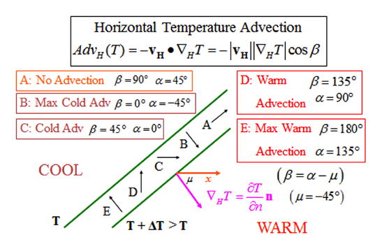
Some examples of simple cases of advection show these concepts (see figure below). When the wind blows along the isotherms, the temperature advection is zero (Case A). When the wind blows from the direction of a lower temperature to a higher temperature (Case B), we have cold-air advection. When the wind blows as some non-normal direction to the isotherms, then we need to multiply the magnitude of the wind and the temperature gradient by the cosine of the angle between them. We can estimate the temperature advection by doing what we did for the gradient, that is, replace all derivatives and partial derivatives with finite $\Delta s$ .

Examples of horizontal temperature advection for cases with different angles between the normal to the isotherms and the wind direction (in math terms). When the temperature gradient and wind direction are parallel, then the advection is maximum; when they are perpendicular, then it is zero. Warm air moving toward cold air will be warm advection; cold air moving toward warm air will be cold advection. Note: v_H used in this figure is the same as U_H in the text.

Credit: H.N. Shirer

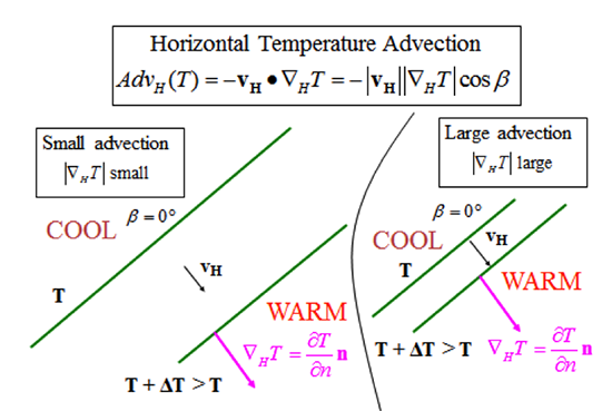
When the isotherms with the same temperature difference are further apart on the map (see figure below), then the horizontal temperature advection will be less than when the isotherms are closer together, if the wind velocity is the same in the two cases.

Examples of horizontal temperature advection for different distances between the isotherms for constant wind velocity. Note: v_H used in this figure is the same as U_H in the text.

Credit: H.N. Shirer

In summary, to calculate the temperature advection, first determine the magnitude and the direction of the temperature gradient. Second, determine the magnitude and direction of the wind. The advection is simply the negative of the dot product of the velocity and the temperature gradient.

Watch this video (2:20) on calculating advection:

Summary and Final Tasks

You now have all of the math tools that you will need to understand the lessons on kinematics and dynamics. For some of you, the concept of partial derivatives is new, but you see how easy it is to apply. We have reviewed vectors and a little vector calculus that you will need in the next few lessons. Dot products and cross products will appear frequently in the next few lessons, so make sure that you are comfortable with them and their applications. We introduced a new operator, the “del” or “gradient” operator, which is essential for describing weather observations and how atmospheric properties vary in space. There are two major coordinate systems that are used to describe atmospheric motion: local Cartesian and spherical. And there are three different coordinates that are used to define the vertical distance starting at Earth’s surface and rising radially: height z (m); pressure or logarithm of pressure p (hPa); and potential temperature $\theta$ (K). You will become skilled in converting between the meteorological wind directions shown on weather maps and in station weather plots and the wind direction needed to do calculations of wind motion and its effects. We introduced the concepts of the Eulerian and Lagrangian frameworks and showed that they are related by advection of a scalar, which is simply the dot product of the wind velocity and the gradient of the scalar.

Once you successfully complete the activities in this lesson, you will be ready to learn about atmospheric kinematics (the description of air movement) and atmospheric dynamics (the study of why air moves the way that it does).