Lesson 9: Kinematics

Overview

The study of kinematics provides a physical and quantitative description of our atmospheric motion, while the study of dynamics provides the physical and quantitative cause-and-effect for this motion. This lesson discusses kinematics.

Global composite infrared satellite image with swirling white clouds

Global composite infrared satellite image for 13 June 2015. The air motion is indicated by the infrared radiation from clouds, which were formed from vertical air motion resulting in cooling.

Credit: NASA Global Hydrology and Climate Center [1]

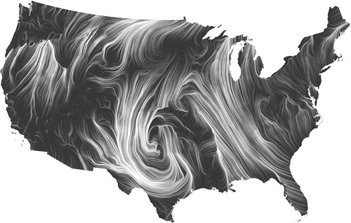
When we look at weather in motion from a satellite, we see very complicated swirls and stretching that evolve over time. We can see the same types of motions on a much smaller scale by observing swirling leaves. These complex motions can be ascribed to combinations of just five different types of atmospheric motion. Quantifying these motions with mathematics, without assigning a cause to the motion, is the focus of this lesson on kinematics.

Learning Objectives

By the end of this lesson, you should be able to:

identify regions of convergence, divergence, positive vorticity, and negative vorticity on a weather map
calculate the strength of the different flow types from observations
relate vertical motion to horizontal convergence and divergence

Questions?

If you have any questions, please post them to the Course Questions discussion forum. I will check that discussion forum daily to respond. While you are there, feel free to post your own responses if you, too, are able to help out a classmate.

9.1 Streamlines and trajectories aren’t usually the same.

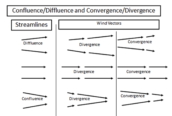
Streamlines are lines that are everywhere parallel to the velocity vectors at a fixed time. They consider the direction of the velocity but not the speed. Sometimes more streamlines are drawn to indicate greater speed, but this is not usually done. Streamlines generally change from one time to the next, giving us “snapshots” of the motion of air parcels. For maps of wind observations for a fixed time, we often look at streamlines. On a map of streamlines, you will see that the lines aren’t always straight and don’t always have the same spacing. Confluence is when streamlines come together. Diffluence is when they move apart.

Wind map of wind streamlines over the continental United States as described in the caption and text above

Wind streamlines over the continental United States. You can see many different examples of confluence (streamlines coming together) and diffluence (streamlines moving apart). See the wind map in motion [2] as a series of streamline maps.

Credit: Creative Commons via Fernanada Viegas and Marten Wattenberg

Trajectories are the actual paths of the moving air parcels, and indicate both the direction and velocity of air parcels over time. Convergence is when the velocity of the air slows down in the direction of the streamline. Divergence is when the velocity of the air speeds up in the direction of the streamline. We will talk more about convergence/divergence later, but for now, you should understand that convergence/divergence come from changes in velocity while confluence/diffluence come from changes in spacing between streamlines.

NOAA HYSPLIT model forecast of wind trajectories as described in the caption

NOAA HYSPLIT model forecast of wind trajectories for June 13, 2015. The top figure is the horizontal view; the bottom figure shows the vertical motion of the trajectories. The distance between squares on individual trajectories indicates 6 hours of travel time. When the squares on a trajectory get closer together with time, there is convergence. When the squares get further apart with time, there is divergence.

Credit: NOAA ARL [3]

Confluence/diffluence and convergence/divergence are illustrated in the figure below:

streamlines: confluence - closer together, diffluence - further apart. Wind vectors: divergence and convergence - get close or further apart

Examples of confluence/diffluence and convergence/divergence.

Credit: H.N. Shirer

Extra Credit Reminder!

Here is another chance to earn one point of extra credit: Picture of the Week!

You take a picture of some atmospheric phenomenon–a cloud, wind-blown dust, precipitation, haze, winds blowing different directions–anything that strikes you as interesting.
Add a short description of the processes that you think are causing your observation. A Word file is a good format for submission.
Use your name as the name of the file. Upload it to the Picture of the Week Dropbox in this week's lesson module. To be eligible for the week, your picture must be submitted by 23:59 UT on Sunday of each week.
I will be the sole judge of the weekly winners. A student can win up to three times.
There will be a Picture of the Week dropbox each week through Lesson 11. Keep submitting entries!

9.2 Watch these air parcels move and change.

satellite image of north america showing water vapor in atmosphere. blue represents water, most over mexico and midwest

Water vapor in the atmosphere over North America showing the behavior of different air parcels as they interact.

Credit: NOAA

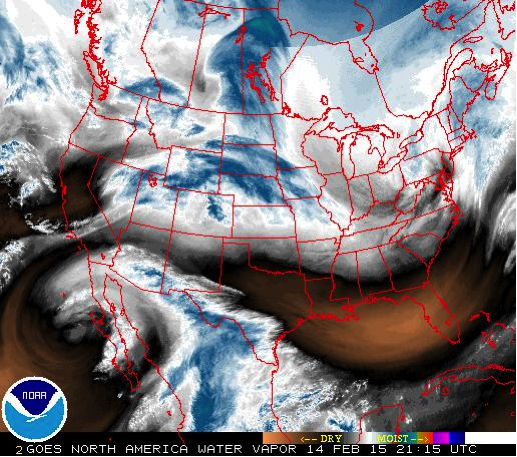
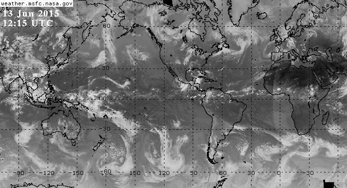
The water vapor image from the GOES 13 satellite, above, indicates different air masses over the United States. As we know from Lesson 7, the water vapor image actually shows the top of a column of water vapor that strongly absorbs in the water vapor channel wavelengths, but it is not a bad assumption to think that there is a solid column of moister air underneath the water vapor layer that is emitting and is observed by the satellite. In a single snapshot, it is not possible to see what happens to the air parcels over time. But if we look at a loop, then we can see the air parcels moving and changing shape as they move.

Watch a Loop

Watch the loop in the animated image below to see. Pick any air parcel with more water vapor in the first frame and then watch it evolve over time. What does it do? Maybe it moves; it spins; it stretches; it shears; it grows. Maybe it does only a few of these things; maybe it does them all.

Enter image and alt text here. No sizes!

Enter caption here

Enter image credit here

We can break each air parcel’s complex behavior down into a few basic types of flows and then mathematically describe them. We will just describe these basic motions here and show how they lead to weather.

An air parcel

Credit: W. Brune

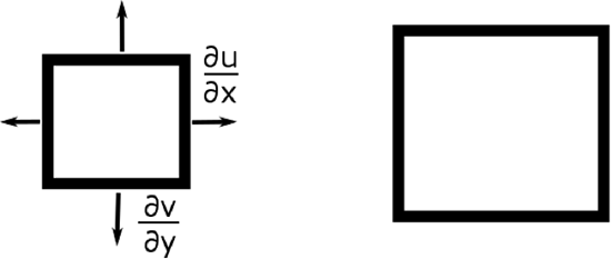
Assume that we have an air parcel as in the figure above. We focus on motion in the two horizontal directions to aid in the visualization (and because most motion in the atmosphere is horizontal) but the concepts apply to the vertical direction as well. If the air parcel is moving and does not change its orientation, shape, or size, then it is only undergoing translation (see figure below).

blue ovals with green and black arrows representing translation as described in caption text.

Air parcel undergoing translation in x-direction (top) and at 45^o (bottom). Black arrows are the wind field; green arrows are the motion of the air parcel. The orientation, shape, and size of the air parcel does not change as it is translated.

Credit: W. Brune

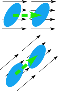
The air parcel can do more than just translate. It can undergo changes relative to translation, and its total motion will then be a combination of translation and relative motion. Let’s suppose that different parts of the air parcel have slightly different velocities. This situation is depicted in the figure below.

blue oval with green arrows on a graph representing two different motion vectors on top & bottom

Air parcel with relative motion for two different points in the air parcel separated by dx in the x direction and dy in the y direction and with different velocities at each point.

Credit: W. Brune, after R. Najjar

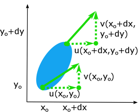
If we consider very small differences dx and dy, then we can write u and v at point (x_o + dx,y_o + dy) as a Taylor series expansion in two dimensions:

\begin{array}{l} u (x_{o} + d x, y_{o} + d y) \approx u (x_{o}, y_{o}) + \frac{\partial u}{\partial x} d x + \frac{\partial u}{\partial y} d y \\ v (x_{o} + d x, y_{o} + d y) \approx v (x_{o}, y_{o}) + \frac{\partial v}{\partial x} d x + \frac{\partial v}{\partial y} d y \\ _______    ___________ \\ translation   relative motion \end{array}

[9.1]

We see that u(x_o,y_o) and v(x_o,y_o) are the translation, and the relative motion is expressed as gradients of u in the x and y directions and gradients of v in the x and y directions.

There are four gradients represented by the four partial derivatives. Each can be either positive or negative for each partial derivative.

\frac{\partial u}{\partial x}

is the following change in velocity in the x direction:

arrows moving away from each other on the x axis >0 arrows moving toward each other <0

\frac{\partial v}{\partial y}

is the following change in velocity in the y direction:

arrows moving away from each other on the y axis >0 arrows moving toward each other <0

\frac{\partial u}{\partial y}

is the following change in velocity in the y direction:

arrows in vertical arrangement on a line, top 2 point right, bottom 2 point left >0, top 2 point left, bottom 2 point right <0

$\frac{\partial v}{\partial x}$ is the following change in velocity in the x direction:

arrows in horizontal arrangement on a line, left 2 point down, right 2 point up >0, left 2 point up, bottom 2 point down <0

Note that a partial derivative is positive if a positive value is becoming more positive or a negative value is becoming less negative. Similarly, a negative partial derivative occurs when a positive value is becoming less positive or a negative value is becoming more negative. Be sure that you have this figured out before you go on.

Watch this video (2:38) for further explanation:

Partials Velocity Distance

Click here for transcript of the Partials Velocity Distance video.

I want to make sure that you understand the partial derivatives of the u and v velocity with respect to x and y because we will soon be using these terms a lot. Let's start with the partial derivative u with respect to x. Consider a constantly increasing x so that the change in x is positive. As x increases, u becomes initially less negative, hence a positive change; then becomes positive, another positive change; and then becomes more positive, another positive change. Since the change in u and the change in x are both always positive, the partial derivative is positive, greater than 0. Look at the case where a partial derivative is less than 0, or negative. As x increases, u becomes less positive hence, a negative change. Then becomes negative, another negative change, then becomes more negative, another negative change. Since the change in u is always negative with a positive change in x, the partial derivative is always negative. Same logic applies to the partial derivative of v with respect to y. Up is positive for y, so you should look at how v changes as y becomes more positive. Look at the case of the change in u with respect to y. It does not matter that u is in the x direction perpendicular to y because we are interested in how u changes as a function of y. Let's look at what happens as y becomes more positive. On the left, u becomes less negative, a positive change in u, then positive, and more positive. Thus the partial derivative is a positive change in u over a positive change in y and therefore is positive, or greater than 0. The change in u with respect to y is always positive in this case. Using the same logic on the right, we see that the change in u with respect to y is always negative. And because a change in y is positive, the partial derivative is negative, or less than 0. The same logic applies to the partial derivative of v with respect to x. To the right is positive for x. So you can determine how v changes as x becomes more positive to see whether the partial derivative is positive or negative.

9.3 Five Air Motion Types You Must Get to Know

Generally, air velocities change with distance in such a way that more than one partial derivative is different from zero at any time. It turns out that any motion of an air parcel is a combination of five different motions, one being translation, which we have already discussed, and four of which can be represented by pairs of partial derivatives of velocity. Of these four, one is a deformation of the air parcel, called stretching, which flattens and lengthens the air parcel. A second is another deformation of the air parcel, called shearing, which twists the air parcel in both the x and y directions. A third is pure rotation, called vorticity. A fourth enlarges or shrinks the parcel without changing its shape, called divergence. Let’s consider each of five types of air motion alone, even though more than one is often occurring for an air parcel.

Translation simply moves the air parcel without stretching it, shearing it, rotating, or changing its area. There are no partial derivatives of velocities involved with translation.

For the remaining four cases, we will provide examples in which the motion (stretching, shearing, vorticity, and divergence) has a positive value. We could have provided examples in which the motion has negative value, but the conclusions would be the same.

Stretching deformation is represented by $\frac{\partial u}{\partial x} - \frac{\partial v}{\partial y}$ . u gets more positive as x gets more positive and u gets more negative as x gets more negative (so that the derivative is always positive), making the parcel grow in the x direction. In the other direction, v gets more negative as y gets more positive and v gets more positive as y gets more negative (so that the derivative is always negative), making the parcel shrink in the y direction (see figure below). However, the total area of the air parcel will remain the same if $\partial u / \partial x = \partial v / \partial y$ . Shown in the figure is positive stretching deformation; negative stretching deformation occurs when the parcel is stretched in the y direction.

box and rectangle representing stretching deformation as described in the text

Stretching deformation. The axis of confluence is in the direction that confluence is occurring; the axis of diffluence is in the direction that diffluence is occurring.

Credit: W. Brune

Shearing deformation is represented by $\frac{\partial v}{\partial x} + \frac{\partial u}{\partial y}$ . In this case, v gets more positive as x gets more positive and v gets more negative as x gets more negative, resulting in the air parcel part at lower x getting pushed towards lower y, and the air parcel part at higher x getting pushed towards higher y. At the same time, u gets more positive as y gets more positive and u gets more negative as y gets more negative, resulting in the air parcel part at lower y getting pushed to lower x and the air parcel part at higher y getting pushed to higher x (see figure below). The total area of the air parcel remains the same after the shearing occurs. Shearing deformation is positive when the air parcel stretches in the southwest/northeast direction and contracts in the southeast/northwest direction (as in the figure below). Shearing deformation is negative when the parcel stretches in the southeast/northwest direction and contracts in the southwest/northeast direction.

box and diamond representing shearing deformation as described in the text

Shearing deformation. The axis of confluence is in the direction that confluence is occurring; the axis of diffluence is in the direction that diffluence is occurring.

Credit: W. Brune

As the two figures above show, both stretching and shearing deformation cause stretching along the axis of diffluence and contraction along the axis of confluence, with the two axes at right angles to each other. These deformations result in weather fronts. In both cases, these motions cause some parts of the air parcel to move away from each other and some parts of the air parcel to move towards each other. The air coming together is called frontogenesis.

Vorticity is represented by $\frac{\partial v}{\partial x} - \frac{\partial u}{\partial y} \equiv ζ$ . Vorticity is special, and because it is special, it is represented by a Greek lower-case letter, zeta (ζ). In this case, the air parcel does not get distorted if $\partial v / \partial x = - \partial u / \partial y$ and does not change area. It simply rotates (see figure below).

square and rotated square to represent vorticity as described in the text

Vorticity. The air parcel simply rotates. In this case, the vorticity is positive and the air parcel is rotating counter-clockwise.

Credit: W. Brune

This difference in partial derivatives may look familiar to you.

\begin{array}{l} {\vec{U}}_{H} = \vec{i} u + \vec{j} v and {\vec{\nabla}}_{H} = \vec{i} \frac{\partial}{\partial x} + \vec{j} \frac{\partial}{\partial y} \\ {\vec{\nabla}}_{H} \times {\vec{U}}_{H} = (\frac{\partial v}{\partial x} - \frac{\partial u}{\partial y}) \vec{k} \\ ζ = \vec{k} \cdot ({\vec{\nabla}}_{H} \times {\vec{U}}_{H}) \end{array}

[9.2]

Vorticity is actually a vector that follows the right-hand rule. Your fingers curve in the direction of the flow and your thumb is the vorticity vector. Here we are discussing only the vertical component of the vorticity. In a right-handed coordinate system, counter-clockwise flow in the x-y plane will result in your thumb pointing in the positive z direction. Hence, vorticity is positive if the rotation is counter-clockwise and is negative if the rotation is clockwise. In the Northern Hemisphere, low-pressure systems are typically characterized by counter-clockwise flow and thus have positive vorticity whereas high-pressure systems are typically characterized by clockwise flow and thus have negative vorticity. The vorticity definition is the same in the Southern Hemisphere (with counter-clockwise flow being positive and clockwise flow being negative), but low-pressure systems usually have clockwise flow and high-pressure systems usually have counterclockwise flow. Vorticity is an important quantity because low- and high-pressure systems are responsible for a lot of weather.

Divergence is represented by $\frac{\partial u}{\partial x} + \frac{\partial v}{\partial y} \equiv δ$ . Divergence is also special, and because it is special, it is represented by a Greek lower-case letter, delta ( $δ$ ). When the divergence is positive, the air parcel grows (i.e., its area increases) (see figure below). If the divergence is negative, then the air parcel shrinks (i.e., its area decreases). Strictly speaking, $δ$ is the horizontal divergence because it describes a change in parcel area projected onto a horizontal plane. Adding ∂w/∂z to the horizontal divergence gives the 3-D divergence.

square and larger square representing divergence as described in the text

Divergence of an air parcel shown for the case when

\partial u / \partial x and \partial v / \partial y

are both positive.

Credit: W. Brune

The divergence can be written in vector notation:

\begin{array}{l} {\vec{U}}_{H} = \vec{i} u + \vec{j} v and {\vec{\nabla}}_{H} = \vec{i} \frac{\partial}{\partial x} + \vec{j} \frac{\partial}{\partial y} \\ {\vec{\nabla}}_{H} \cdot {\vec{U}}_{H} = \frac{\partial u}{\partial x} + \frac{\partial v}{\partial y} \end{array}

[9.3]

Watch this video (1:56) for further explanation:

Five Air Motion Types

Click here for transcript of the Five Air Motion Types video.

Airflow can be characterized by a combination of five basic flow types. Translation, which is just a motion of the air parcel, no change in area. Stretching deformation, which increases the parcel in one direction and decreases it in another. Shearing deformation, which shears the air parcel simultaneously in the x and y directions, creating a diamond shape out of a square. Vorticity, which thins the air parcel. And divergence, which grows the air parcel. The last four types can be represented by combinations of the partial derivatives of horizontal velocities, u and v, with respect to horizontal directions, x and y. Note that if we know the wind velocity vectors in the [INAUDIBLE] grid then we can calculate these five wind types for an airflow by determining the changes in the velocities as functions of x and y. And then combining these differentials that are shown here to find the actual values for stretching deformation, shearing deformation, vorticity, and divergence. The units for all of these motion types is per second, which is a frequency. In the figures, I have shown only those transformations that are positive. Negative translation goes to the left. Negative stretching deformation elongates the parcel in the y direction. Negative sharing deformation elongates the parcel in the northwest-southeast direction. Negative vorticity is clockwise. Negative divergence causes the air parcel to shrink, which is called convergence. Prove it to yourself that these transformations shown here are all possible. We will use the divergence heavily in the next section to the lesson.

9.4 How does divergence relate to the air parcel’s area change?

We see that divergence is positive when the parcel area grows and is negative when it shrinks. We call growth “divergence” and shrinking “convergence.” We wish to know whether air parcels come together (converge) or spread apart (diverge) or if the parcel area increases with time (divergence) or decreases with time (convergence).

Let’s see how divergence in the horizontal two dimensions is related to area change. We can do a similar analysis that relates divergence in three dimensions to a volume change, but we will stay with the two-dimensional case because it is easier to visualize and also has important applications. Consider a box with dimensions Δx and Δy. Different parts of the box are moving at different velocities (see figure below).

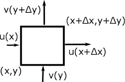
A box that is moving at greater velocity for parts that are at greater x and greater y.

Credit: W. Brune

The box's area, A, is given by:

$\begin{array}{l} A = Δ x Δ y \\ \frac{d A}{d t} = \frac{d (Δ x Δ y)}{d t} = Δ x \frac{d (Δ y)}{d t} + Δ y \frac{d (Δ x)}{d t} = \\ Δ x [v (y + Δ y) - v (y)] + Δ y [u (x + Δ x) - u (x)] \\ divide by A = Δ x Δ y \\ \frac{1}{A} \frac{d A}{d t} = \frac{v (y + Δ y) - v (y)}{Δ y} + \frac{u (x + Δ x) - u (x)}{Δ x} \\ Let Δ y \to 0, Δ x \to 0 \\ \frac{1}{A} \frac{d A}{d t} = \frac{\partial u}{\partial x} + \frac{\partial v}{\partial y} = {\vec{\nabla}}_{H} • {\vec{U}}_{H} \end{array}$

So we see that the fractional change in the area is equal to the horizontal divergence. Note that the dimension of divergence is time^–1 and the SI unit is s^–1.

We can do this same analysis for motion in three dimensions to get the equation:

$\frac{1}{V} \frac{d V}{d t} = \frac{\partial u}{\partial x} + \frac{\partial v}{\partial y} + \frac{\partial w}{\partial z} = {\vec{\nabla}}_{H} \cdot {\vec{U}}_{H} + \frac{\partial w}{\partial z} = \vec{\nabla} \cdot \vec{U}$

[9.4]

where V is the parcel volume. Thus, the 3-D divergence is just the fractional rate of change of an air parcel’s volume.

Check Your Understanding

Suppose that an air parcel has an area of 10,000 km² and it is growing by 1 km² each second. What is its divergence?

Click for answer.

$\frac{Δ A}{Δ t} = 1 {km}^{2} s^{- 1}$ , so $(\frac{1}{A}) (\frac{Δ A}{Δ t}) = (\frac{1}{10^{4}} {km}^{2}) (1 {km}^{2} s^{- 1}) = 10^{- 4} s^{- 1}$ .

Suppose that an air parcel has a area of 10,000 km² and has a divergence of –10^–4 s^–1. Is the air parcel growing or shrinking?

Click for answer.

$divergence = δ = (\frac{1}{A}) (\frac{Δ A}{Δ t})$ , or $\frac{Δ A}{A} = δ Δ t = (- 10^{- 4} s^{- 1}) (1 s) = - 10^{- 4}$ . The air parcel is shrinking.

Check out this video (1:33) for further explanation:

Divergence Area

Click here for transcript of the Divergence Area video.

We can use a very simple demonstration to show how differences in velocity from one end of an air parcel to the other can cause changes in area. Let's let this be our air parcel here, outlined in the dark blue. Several things can happen to this air parcel. One, it can translate. So it can just move with a certain velocity across from left to right. The second thing it can do is it can have a zero velocity here and have a higher velocity here on this end. And it can then grow. And so you see that the area is increasing as time goes on. So we can combine these two motions and see what happens. And so we have some velocity at the parcel, but we have a greater velocity on the right hand side. And we see that as it moves, it grows. It's also possible that as it moves, it shrinks because the velocity on this side is less than the velocity on this side. Then as it moves along, you will see that actually the area's contracting. We can do the same sort of analysis in the y direction. And from this, we can show that in fact, the difference in velocity from here to here can result in the growth or the shrinking of the area of the parcel.

Quiz 9-1: The way the wind blows.

Find Practice Quiz 9-1 in Canvas. You may complete this practice quiz as many times as you want. It is not graded, but it allows you to check your level of preparedness before taking the graded quiz.
When you feel you are ready, take Quiz 9-1. You will be allowed to take this quiz only once. Good luck!

9.5 How is the horizontal divergence/convergence related to vertical motion?

Composite of satellite infrared image overlaid with surface analysis and radar for united states

Composite of satellite infrared image overlaid with surface analysis and radar. Note that the precipitation is generally associated with the low-pressure regions and the high-pressure areas are generally free of significant clouds. As we will soon see, low-level air converges into low-pressure regions, causing uplift, which causes clouds and precipitation. Low-level air diverges from high-pressure regions, causing downwelling air and warming and drying by adiabatic descent.

Credit: Unisys

Our goal here is to relate horizontal convergence and divergence to vertical motion. If vertical motion is upward, then the uplifted air will cool, clouds will form, and it might rain or snow. If vertical motion is downward, then the downwelling air will warm by adiabatic descent, clouds will evaporate, and it will become clear.

To find out what will happen, we need to go back to a fundamental law of mass conservation [4], which we will derive in detail in Lesson 10. Here we simply quote the result:

\frac{1}{ρ} \frac{D ρ}{D t} + \vec{\nabla} • \vec{U} = 0

where $ρ$ is the density and D/Dt is the total derivative.

For divergence, $\vec{\nabla} • \vec{U} > 0$ , volume increases and density must decrease to conserve mass.

For convergence, $\vec{\nabla} • \vec{U} < 0$ , volume decreases and density must increase to conserve mass.

However, to good approximation, density does not change with time for any given horizontal surface. Sure, density decreases exponentially with height, but for each height level, the density at that level is fairly constant.

So, to a good approximation:

\vec{\nabla} • \vec{U} = 0

and because we can separate out the horizontal and vertical components of divergence:

\vec{\nabla} • \vec{U} = {\vec{\nabla}}_{H} • {\vec{U}}_{H} + \frac{\partial w}{\partial z}

we see that:

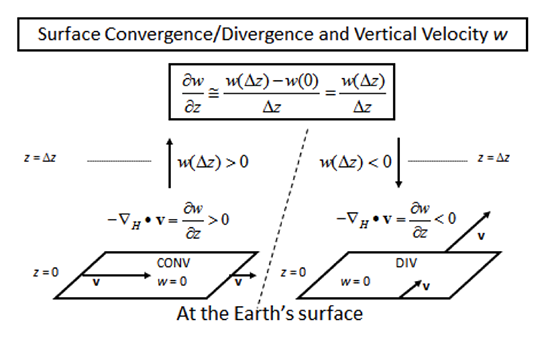
{\vec{\nabla}}_{H} • {\vec{U}}_{H} + \frac{\partial w}{\partial z} = 0, or \frac{\partial w}{\partial z} = - {\vec{\nabla}}_{H} • {\vec{U}}_{H}

[9.5]

Thus, horizontal divergence is compensated by vertical convergence and horizontal convergence is compensated by vertical divergence.

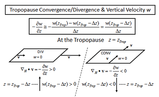
{\vec{\nabla}}_{H} • {\vec{U}}_{H} > 0 means \frac{\partial w}{\partial z} < 0

Horizontal divergence gives a decrease in vertical velocity with height.

{\vec{\nabla}}_{H} • {\vec{U}}_{H} < 0 means \frac{\partial w}{\partial z} > 0

Horizontal convergence gives an increase in vertical velocity with height.

Now, in the troposphere, the vertical velocity is close to zero (w ~ 0) at two altitudes. The first is Earth’s surface, which forms a solid boundary that stops the vertical wind. The second is the tropopause, above which the rapid increase in stratospheric potential temperature strongly inhibits vertical motion from the troposphere (see two figures below), so much so, that we can say that the vertical wind must be ~ 0 at the tropopause.

diagram of surface convergence/divergence and vertical velocity as described in the text

Surface convergence or divergence and the resulting vertical velocity (note: v used in this figure is the same as U_H in the text.).

Credit: H.N. Shirer

diagram of tropopause convergence/divergence and vertical velocity as described in the text

Tropopause convergence or divergence and the resulting vertical velocity (note: v used in this figure is the same as U_H in the text.).

Credit: H.N. Shirer

These processes can be summarized in the following table:

plane	process	surface area change	∂w/∂z	w
surface	convergence	decrease	+	up
surface	divergence	increase	–	down
aloft	convergence	decrease	+	down
aloft	divergence	increase	–	up

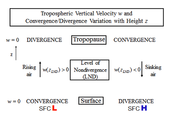
Let’s now consider the effect that divergence/convergence aloft has on surface convergence/divergence (see figure below).

Divergence aloft is associated with rising air throughout the troposphere, which is associated with low pressure and convergence at the surface.

Convergence aloft is associated with sinking air throughout the troposphere, which is associated with high pressure at the surface and thus divergence at the surface.

So, starting at the surface, the vertical velocity becomes more positive with height when there is surface convergence, reaches some maximum vertical velocity, and then becomes less positive with height again toward the divergence aloft.

Similarly, starting again at the surface, the vertical velocity becomes more negative with height when there is surface divergence, reaches some maximum negative velocity, and then becomes less negative with height again near convergence aloft.

shows how divergence aloft causes low surface pressure/convergence & how convergence aloft causes high surface pressure & divergence

How divergence aloft connects to surface low pressure and convergence and how convergence aloft connects to surface high pressure and divergence.

Credit: H.N. Shirer

Now watch this video (3:52) on horizontal divergence:

Horizontal Divergence Vertical Motion

Click here for transcript of the Horizontal Divergence Vertical Motion video.

The key concepts that allow horizontal divergence to be converted into vertical motion are that mass is conserved, but the air density and density vertical structure are fairly constant with time, and that the vertical wind at Earth's surface and at the tropopause is effectively 0. This means that the total divergence must be approximately 0 so that the air parcel volume remains constant. Thus, changes in the horizontal area cause changes in the vertical height to maintain the air quality. A key to remember is that the vertical velocity w is partial derivative with respect to height z do not always have the same sign. The second key point to remember is that the partial derivative of w with respect to z is a negative divergence. We would look first at diverging mirror surface. But if there is horizontal convergence, then the air must go somewhere, and it cannot go down, so it goes up. The equation actually says that the partial derivative of w, the vertical velocity with respect to z, must be positive. But if w equals 0 at Earth's surface and w is increasingly with altitude, than w must be positive. For divergence near Earth's surface, we see that the partial derivative of w with respect to z is negative, which means that w must be negative above the surface since w equals 0 at earth's surface. So the air velocity w must be downward. But the tropopause, the rapid increase in stress for potential temperature acts like a lid on the troposphere. Effectively makes w go to 0 at the tropopause. There is a horizontal divergence aloft then w must be upward to maintain the air parcel volume as the air parcel spreads out horizontally near the tropopause. Mathematically, this means that w must be positive. But we know that it must go to 0 tropopause. Therefore, the partial of w with respect to z must be negative as it approaches the tropopause, i.e. w is decreasing with increasing height to 0 at the tropopause from a positive value in the troposphere. On the other hand, if there is convergence in the air near the tropopause then, the air must go down and the vertical velocity w must be negative. If we look at the changes in w with respect to height above the level of non-divergence, as z increases, w goes from more negative to less negative, which is a positive change in w, with a positive change in z. So the partial derivative is positive even though w is negative. Putting these pieces together, we see that if we have convergence at Earth's surface, which occurs in low pressure areas for reasons we will see in lesson 10, then at the tropopause, there's divergence. In between the two surfaces the velocity is upward-- that is, w is positive. If we have a divergence near Earth's surface, which occurs in high pressure areas, then there is convergence at the tropopause. In between, the vertical velocity is downward. That is, w is negative. The outward moving air above low pressure creates cooling, which leads to clouds and precipitation. The downward moving air above high pressure region causes warming and drying, resulting in clear conditions.

Surface map of weather for February 2, 2015. Precip on east coast

Surface map of weather for February 2, 2015. Fronts, lows, and highs are indicated. Radar shows where precipitation is falling.

Credit: Unisys

Weather map of the United States for February 2, 2015. Analysis for the 500 hPa pressure surface (about 5 km altitude), with isopleths, wind vectors, and enhanced relative humidity.

500 mb weather map for February 2, 2015. Black lines are surface heights and wind barbs show the direction and magnitude of wind.

Credit: NOAA.

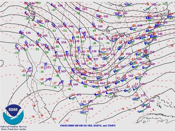
We have shown that convergence and divergence aloft near the tropopause is related to surface highs and lows. Now it's your turn to find some examples. Go to a source of information about surface pressure and upper-air winds and pick out some regions that show this relationship. One good source is the Penn State e-Wall [5], for which you can use the "U.S. Satellite Overlays."

9.6 How fast is the vertical wind and which way does it blow?

What are typical values of the vertical velocity caused by convergence or divergence and how do they vary with height? The vertical velocity, w, is typically too small to measure by a radiosonde. But we can estimate w from the convergence/divergence patterns:

\frac{\partial w}{\partial z} = - {\vec{\nabla}}_{H} • {\vec{U}}_{H} = - δ

Note that this equation just gives the derivative of the vertical velocity, not the vertical velocity itself. So to find the vertical velocity, we must integrate both sides of the equation over height, z.

Integrate this equation from the surface (z = 0) to some height z:

{\int^{​}}^{​}_{0}^{z} \frac{\partial w}{\partial z'} d z' = - {\int^{​}}^{​}_{0}^{z} δ d z'

w (z) = - {\int^{​}}^{​}_{0}^{z} δ d z'

[9.6]

where we have assumed that w(0) is equal to zero, which is true if the surface is horizontal. Equation [9.6] gives the kinematic vertical velocity.

To a good approximation, it has been determined that divergence/convergence for horizontal flow at large scales (e.g., synoptic scales, ~1000 km) varies linearly with altitude.

δ = δ_{s} + b z

[9.7]

where δ_s is the surface divergence and b is a constant. Substituting this expression for the horizontal divergence into Equation [9.6], we get:

w (z) = - {\int^{​}}^{​}_{0}^{z} δ d z^{'} = - δ_{s} z - \frac{1}{2} b z^{2}

[9.8]

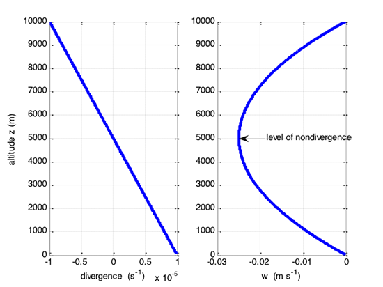
The trick is to find b using some other information. To find b, note that the derivative $\frac{\partial w}{\partial z}$ must equal 0 at some level because w must be 0 at both Earth's surface and the tropopause while, in general, w is non-zero elsewhere. If, for example, the derivative is negative near Earth's surface, it must become positive at the tropopause in order for w to go to zero at the tropopause. Therefore, at some level in between being negative in the lower troposphere and positive in the upper troposphere, the derivative must be zero. We call this level the level of nondivergence, z_LND, and can use it to find an expression for w as a function of z by setting the divergence equal to zero in Equation [9.7]:

0 = - δ_{s} - b z_{L N D}, or b = - \frac{δ_{s}}{z_{L N D}}

[9.9]

w (z) = - δ_{s} z + \frac{δ_{s}}{2 z_{L N D}} z^{2}

[9.10]

The large-scale surface divergence typically has a value of 10^–5 s^–1. The large-scale level of nondivergence is typically about 5000 m. So, a typical value for b is:

b = - \frac{δ_{s}}{z_{L N D}} = - \frac{10^{- 5} s^{- 1}}{5000 m} = - 2 \times 10^{- 9} m^{- 1} s^{- 1}

So, for typical large-scale surface divergence:

w (z) = (- 10^{- 5} s^{- 1}) z + (10^{- 9} m^{- 1} s^{- 1}) z^{2}

At $z = z_{L N D} = 5000 m, w (z_{L N D}) = - 2.5 {cm s}^{- 1} = (- 2.5 \times 10^{- 5} {km s}^{- 1}) (86400 {s day}^{- 1}) = - 2.2 {km day}^{- 1}$ (see figure below).

The result is that w is only a few cm s^–1. In a day, the air mass can rise or fall only a few kilometers. Compare this vertical motion dictated by large-scale convergence and divergence to the vertical motion in the core of a powerful thunderstorm (horizontal scale of a few km), where the vertical velocities can be many m s^–1. This simple model is called the bowstring model because the shape of the vertical velocity looks like a bowstring that is fixed at two points but can vary as a parabola in between.

graph showing Divergence and vertical wind, see caption

Divergence (left) and vertical wind (right). For convergence aloft (negative divergence), the vertical wind is negative with a maximum value near 5000 m and remains negative as it decreases toward zero at the surface, where there is divergence (positive divergence) near the surface.

Credit: W. Brune

Quiz 9-2: Connecting the dots with vertical motion.

Find Practice Quiz 9-2 in Canvas. You may complete this practice quiz as many times as you want. It is not graded, but it allows you to check your level of preparedness before taking the graded quiz.
When you feel you are ready, take Quiz 9-2. You will be allowed to take this quiz only once. Good luck!

Summary and Final Tasks

Kinematics describes the behavior of atmospheric motion but not the cause. Streamlines provide snapshots of that motion and trajectories show where individual air parcels actually go. All atmospheric motion in the horizontal is made up of one or more of five distinct types of motion: translation, stretching deformation, shearing deformation, vorticity, and divergence. Stretching and shearing deformation lead to the formation or the dissolution of surface weather fronts. Vorticity describes the counter-clockwise rotation around low pressure (in the Northern Hemisphere) and clockwise rotation around high pressure (in the Northern Hemisphere) and is thus associated with much of weather. Divergence/convergence aloft leads to vertical winds that connect to convergence/divergence at the surface, and through this mechanism, air motion aloft communicates with air motion at the surface.

This lesson showed the mathematics necessary to quantify all of these processes. So besides identifying streamline confluence/diffluence, you practiced quantifying the five flow types from weather maps of streamlines with wind vectors. Finally, you calculated the vertical wind and its direction (up or down) based on the divergence/convergence of the winds aloft.

Reminder - Complete all of the Lesson 9 tasks!

You have reached the end of Lesson 9! Double-check that you have completed all of the activities before you begin Lesson 10.