Lesson 1- Introduction to Climate and Climate Change
Introduction
Did you complete the Course Orientation?
Before you begin this course, please complete the Course Orientation.
About Lesson 1
Human-caused climate change represents one of the great environmental challenges of our time. To appreciate its societal, environmental, and economic implications, one must appreciate the basic underlying science. This course seeks to first lay down the fundamental scientific principles behind climate change and global warming. These principles involve aspects of atmospheric science and meteorology, as well as aspects of other areas of the physical and biological sciences. With a firm grounding in the basic science, we go on to explore other issues involving climate change impacts and the issue of mitigation — that is, solutions to dealing with the challenges presented by climate change.
In the process, we will learn how to do basic computations and to use theoretical models of the climate system of varying complexity to address questions regarding future climate change. Students will explore the impacts of various alternative greenhouse gas emissions scenarios and investigate policies that would allow for appropriate stabilization of future greenhouse gas concentrations. The structure of the course roughly parallels the treatment of the subject matter by the reports of the Intergovernmental Panel on Climate Change (IPCC), focusing first on the basic science, then the future projections and their potential impacts, and finally issues involving adaptation, vulnerability, and mitigation. We will use a variety of tools to inform our understanding of these topics, including digital video, audio, simulation models, and virtual field trips to online data resources.
In this first lesson, we are going to define climate and climate change, as well as the closely related matter of global warming. We will introduce the components of the climate system (the atmosphere, ocean, cryosphere, and biosphere). We will also briefly introduce some of the other key scientific concepts: atmospheric structure and composition, energy balance, atmospheric and oceanic circulation. We will draw a distinction between natural and human impacts on climate, and we will review the science behind greenhouse gases and the greenhouse effect. We will explore the crucial topic of feedback mechanisms, including important emerging knowledge regarding carbon cycle feedbacks. Finally, we will begin to explore a number of important overriding themes, such as the role of scientific uncertainty in decision making.
What will we learn in Lesson 1?
By the end of Lesson 1, you should be able to:
- Define the Earth's climate system and its components;
- Distinguish the factors governing natural climate variability from human-caused climate change;
- Explain the greenhouse effect;
- Describe the role of feedback mechanisms; and
- Discuss the role of uncertainty in decision-making.
What will be due for Lesson 1?

Please refer to the Syllabus for the specific time frames and due dates.
The following is an overview of the required activities for Lesson 1. Detailed directions and submission instructions are located within this lesson.
- Read:
- IPCC Sixth Assessment Report, Working Group 1
- Summary for Policy Makers
- Introduction: p. 4
- The Current State of the Climate: p. 4-11
- Summary for Policy Makers
- Dire Predictions, v.2: p. 8, 12-13, 22-25
- IPCC Sixth Assessment Report, Working Group 1
- Participate in the LESSON 1: GENERAL DISCUSSION OF METEO 469 discussion forum.
What is Climate?
When it comes to defining climate, it is often said that "climate is what you expect; weather is what you get". That is to say, climate is the statistically-averaged behavior of the weather. In reality, it is a bit more complicated than that, as climate involves not just the atmosphere, but the behavior of the entire climate system—the complex system defined by the coupling of the atmosphere, oceans, ice sheets, and biosphere.
Having defined climate, we can begin to define what climate change means. While the notion of climate is based on some sort of statistical average of behavior of the atmosphere, oceans, etc., this average behavior can change over time. That is to say, what you "expect" of the weather is not always the same. For example, during El Niño years, we expect it to be wetter in the winter in California and snowier in the southeastern U.S., and we expect fewer tropical storms to form in the Atlantic during the hurricane season. So, climate itself varies over time.
If climate is always changing, then is climate change by definition always occurring? Yes and No. A hundred million years ago, during the early part of the Cretaceous period, dinosaurs roamed a world that was almost certainly warmer than today. The geological evidence suggests, for example, that there was no ice even at the North and South poles. So global warming can happen naturally, right? Certainly, but why was the Earth warmer at that time?
A hint of why can be found in many of the careful renditions of what the Earth may have looked like during the age of dinosaurs. Some of the most insightful interpretations came from the 19th century Yale paleontologist, Othniel Charles Marsh. Let us look at one of his renderings:
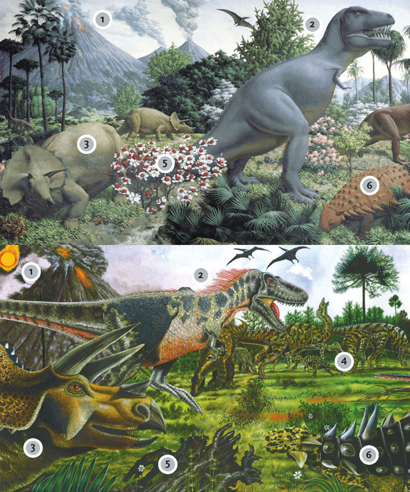
Think About It!
What features of the above mural might provide a clue for why the early Cretaceous was so warm?
As we will see later in this lecture, volcanic eruptions have had a cooling impact on climate on a historical time frame, by injecting reflecting aerosols into the atmosphere, which block out some amount of incoming sunlight for several years after the eruption. However, over millions of years, volcanic eruptions have a different, and indeed quite profound, influence on the atmospheric composition. They pump carbon dioxide into the atmosphere. More carbon dioxide means a stronger greenhouse effect. We will talk about this later in the lecture.
So, the major climate changes in Earth's geologic past were closely tied to changes in the greenhouse effect. Those changes were natural. The changes in greenhouse gas concentrations that we talk about today, are, however, not natural. They are due to human activity.
Importance: Why Should We Care About Climate Change?
As we have discussed, climate change can be natural. If climate changes naturally, then why should we be concerned about the climate change taking place today? After all, the early Cretaceous period discussed previously was warmer than today, but life thrived even in regions, such as the interior of Antarctica, that are uninhabitable today.
One misconception is that the threat of climate change has to do with the absolute warmth of the Earth. That is not, in fact, the case. It is, instead, the rate of change that has scientists concerned. Living things, including humans, can easily adapt to substantial changes in climate as long as the changes take place slowly, over many thousands of years or longer. However, adapting to changes that are taking place on timescales of decades is far more challenging.
Here is a useful "thought experiment" to illustrate what sort of discussion might be happening now if, instead of the current climate, we were living under the climate conditions of the last Ice Age, and human fossil fuel emissions were pushing us out of the ice age and into conditions resembling the pre-industrial period, rather than the actual case, where we are pushing the Earth out of the pre-industrial period and into a period with conditions more like the Cretaceous. Take a look at Figure 1.2 below, which indicates the Gulf coast continental outline near the height of the last Ice Age 18,000 years ago, vs. the current continental outline.
Everything in the lighter shading would be flooded in the transition from the ice age to pre-industrial modern climate. But what sort of effort would that have taken?
It turns out that the natural increase in atmospheric CO2 that led to the thaw after the last Ice Age was an increase from 180 parts per million (ppm) to about 280 ppm. This was a smaller increase than the present-time increase due to human activities, such as fossil fuel burning, which thus far have raised CO2 levels from the pre-industrial value of 280 ppm to a current level of over 400 ppm--a level which is increasing by 2 ppm every year. So, arguably, if the dawn of industrialization had occurred 18,000 years ago, we may very likely have sent the climate from an ice age into the modern pre-industrial state.
How long it would have taken to melt all of the ice is not precisely known, but it is conceivable it could have happened over a period as short as two centuries. The area ultimately flooded would be considerably larger than that currently projected to flood due to the human-caused elevation of CO2 that has taken place so far. The hypothetical city of "Old Orleans" would have to be relocated from its position in the Gulf of Mexico 100+ miles off the coast of New Orleans, to the current location of "New Orleans".
By some measures, human interference with the climate back then, had it been possible, would have been even more disruptive than the current interference with our climate. Yet that interference would simply be raising global mean temperatures from those of the last Ice Age to those that prevailed in modern times prior to industrialization. What this thought experiment tells us is that the issue is not whether some particular climate is objectively "optimal". The issue is that human civilization, natural ecosystems, and our environment are heavily adapted to a particular climate — in our case, the current climate. Rapid departures from that climate would likely exceed the adaptive capacity that we and other living things possess, and cause significant consequent disruption in our world.
So, hopefully, we have established that climate change is something worth caring about. Perhaps it is something worth doing something about. But you cannot really do anything about a problem that you do not understand, let alone know how to solve.
In the remainder of this lesson, we are going to try to begin to get a handle on the fundamental science underlying climate change and global warming.
Overview of the Climate System - Part 1
The Components of the Climate System
The climate system reflects an interaction between a number of critical sub-systems or components. In this course, we will focus on the components most relative to modern climate change: the atmosphere, hydrosphere, cryosphere, and biosphere. Please watch the following video to walk through the important aspects of these components.
Video: The Components of the Climate System (1:52)
PRESENTER: This is a schematic of the climate system. We can think of the climate as representing essentially four subsystems that are coupled together.
Among those subsystems are the atmosphere-- so that's one of the spheres. And that, of course, represents the chemistry and the dynamics of that component of the system, the atmosphere.
Then we have the hydrosphere, which is all the water that exists on the face of the earth in liquid form. So that would be the oceans and seas, rivers, lakes, et cetera. Water that exists in vapor form-- water vapor-- is part of the atmosphere.
Then we have the cryosphere, which is all of the water that exists in the form of snow and ice. That would include mountain glaciers, that would include the major ice sheets, and that would include snow that falls in the extra tropics during the winter.
Finally, then we have the biosphere, and that represents all living things on the face of the earth. And as we'll see in this course, the biosphere does indeed play a key role. It influences the composition of the atmosphere through the global carbon cycle, it influences the surface characteristics of the land, which has implications for climate.
So ultimately what we have are these four systems-- the hydrosphere, the atmosphere, the cryosphere, and the biosphere-- interacting with each other to form what we call the climate system PRESENTER: I think that this course fits into the major, energy and sustainability of policy, in a very vital way. I mean, climate change, in a sense, is sort of the 800-pound gorilla when it comes to the future energy policy. We need to take into account the fact that there are impacts, and there will continue to be impacts, that will grow in magnitude if we continue on our course of deriving energy from fossil fuel burning.
Decision-making ultimately relies upon taking both costs and benefits into account, and with climate change, there are costs, and many of those costs lie in our future. And in order to make appropriate decisions about how we balance the benefits of the energy that we can get today relatively cheaply from burning fossil fuels with the cost to society and to our environment of our continued reliance on fossil fuel burning, to really take on that big question, we need to understand the basics of climate change.
What is it about? What's causing it? What are the impacts, and what are the likely costs of future climate change? And how do we take into account these costs and benefits in making actual decisions about our energy future? So, hopefully, by the time this course is done, we will have brought all of those things together in a way that students can now think about this problem in a way that they wouldn't have been able to before they took the course.
Atmospheric Structure and Composition
The atmosphere is, of course, a critical component of the climate system, and the one we will spend the most time talking about.
One key feature about the atmosphere is the fact that pressure and density decay exponentially with altitude:
As you can see, the pressure decays nearly to zero by the time we get to 50 km. For this reason, the Earth's atmosphere, as noted further in the discussion below, constitutes a very thin shell around the Earth.
The exponential decay of pressure with altitude follows from a combination of two very basic physical principles. The first physical principle is the ideal gas law. You are probably most familiar with the form , but that form applies to a bounded gas, where the volume can be defined. In our case, the gas is free, and the appropriate form of the ideal gas law is
where is the atmospheric pressure, is the density of the atmosphere, is the gas constant that is specific to Earth's atmosphere, and is temperature.
The 2nd principle is the force balance. There are two primary vertical forces acting on the atmosphere. The first is gravity, while the other is what is known as the pressure gradient force — it is the support of one part of the atmosphere acting on some other part of the atmosphere. This balance is known as the hydrostatic balance.
The relevant pressure gradient force in this case is the vertical pressure gradient force. When we are talking about a continuous fluid (which the atmosphere or ocean is), then the correct form of force balance involves force per unit volume of fluid.
In this form, we have for gravity (the negative sign indicates a downward force):
where is Earth's surface gravitational acceleration ( ).
The pressure gradient force has to be written in terms of a derivative:
The positive sign ensures that an atmosphere with a greater density below exerts a positive (upward) force.
In equilibrium, these forces must balance, i.e.
Now we can use the ideal gas law (eq. 1.) to substitute for ρ, the expression , giving
or re-arranging a bit,
The term in parentheses can be treated as a constant (in reality, temperature varies with altitude, but it varies less dramatically than pressure or density, so it's easiest to simply treat it as a constant).
This is a relatively simple first order differential equation.
Self Check...
Do you remember how to solve this first order differential equation from your previous math studies?
Click for answer.
Or, we can exponentiate both sides to yield:
The expression for atmospheric pressure as a function of altitude is:
where is the surface pressure, and is the surface height (by convention typically taken as zero).
This equation is known as the hypsometric equation.
The combination has units of inverse length, and so we can define a scale height (assuming a mean temperature ,
and write:
this gives an exponential decline of pressure with height, with the e-folding height equal to the scale height, representing the altitude at which pressure falls to roughly 1/3 of its surface value. At this altitude, which as you can see from the above graphic is just a bit below the height of Mt. Everest, roughly 2/3 of the atmosphere is below you.
Self-check...
Using the hypsometric equation (9 above), estimate the altitude at which roughly half of the atmosphere is below you.
Click for answer.
Take logs of both sides and rearrange:
Take and use from earlier:
Let us look at the vertical structure of the atmosphere in more detail, define some key layers of the atmosphere:
Video: Key Layers of the Atmosphere (2:41)
PRESENTER: We're going to-- OK. Well, let's talk a little bit about Earth's atmosphere. Here we're viewing Earth from outer space. And we can see there's this faint blue shell encasing the planet. And that faint blue shell is indeed Earth's atmosphere. So this gives us a sense of how relatively thin Earth's atmosphere actually is.
As it turns out, the lower 80 kilometers-- so that is, the first 80 kilometers above the Earth's surface-- contains just about 99% of the atmosphere. So the atmosphere really is this thin blue shell around the Earth.
Now, we can further decompose the atmosphere into various layers. The lowest of these layers is what we call the troposphere. Depending on the latitude, it's somewhere between the first 10 and 14 kilometers. And it's the area of the atmosphere within which we reside, in which most of Earth's surface resides-- in fact, all of Earth's surface, even the tallest mountains. It's also the layer within which weather takes place.
Now, this plot here shows temperature as a function of altitude. And we can see that, within the troposphere, temperatures decrease. It turns out they decrease at a rate of about 6 and 1/2 degrees Celsius per kilometer. And they continue to do so until we reach this boundary here between the troposphere and the next layer up, the stratosphere, where that temperature trend reverses and temperatures, in fact, start to increase as we go up further in the atmosphere. The boundary between these two layers is what we call the tropopause.
Now, why do temperatures increase as we get into the stratosphere? Well, it has to do with the chemistry of the atmosphere. And in fact, the existence of ozone within the stratosphere-- it's the photodissociation of ozone by solar radiation and the heat given off during that photodissociation process that actually heats the stratosphere and leads to the increasing temperatures as we go up in the atmosphere.
Now primarily, in this course, we are going to focus on the troposphere and to some extent the stratosphere. Those are the main parts of the atmosphere that we're going to be interested in.
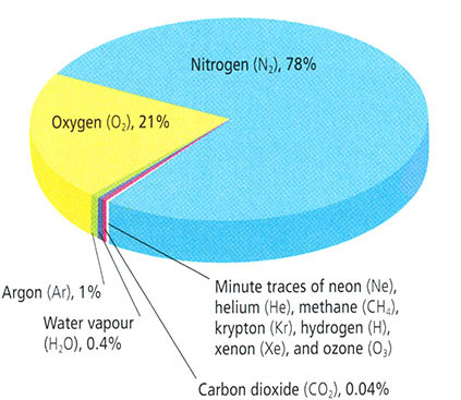
- Nitrogen (N2), 78%
- Oxygen (O2), 21%
- Argon (Ar), 1%
- Water vapor (H2O), 0.4%
- Carbon dioxide (CO2), 0.04%
- Minute traces of: neon (Ne), helium (He), methane (CH4), krypton (Kr), hydrogen (H), xenon (Xe), and ozone (O3)
© 2015 Pearson Education, Inc.
Now, let us talk a bit more about the atmospheric composition:
The atmosphere is mostly nitrogen and oxygen, with trace amounts of other gases. Most atmospheric constituents are well mixed, which is to say, these constituents vary in constant relative proportion, owing to the influence of mixing and turbulence in the atmosphere. The assumption of a well-mixed atmosphere and the assumption of ideal gas behavior, were both implicit in our earlier derivation of the exponential relationship of pressure with height in the atmosphere.
There are, of course, exceptions to these assumptions. As discussed earlier, ozone is primarily found in the lower stratosphere (though some is produced near the surface as consequence of photochemical smog). Some gases, such as methane, have strong sources and sinks and are therefore highly variable as a function of region and season.
Atmospheric water vapor is highly variable in its concentration, and, in fact, undergoes phase transitions between solid, liquid, and solid form during normal atmospheric processes (i.e., evaporation from the surface, and condensation in the form of precipitation as rainfall or snow). The existence of such phase transitions in the water vapor component of the atmosphere is an obvious violation of ideal gas behavior!
Of particular significance in considerations of atmospheric composition are the so-called greenhouse gases (CO2, water vapor, methane, and a number of other trace gases) because of their radiative properties and, specifically, their role in the so-called greenhouse effect. This topic is explored in greater detail later on in this lesson.
Overview of the Climate System (part 2)
Basics of Energy Balance and the Greenhouse Effect
An interactive animation provided below allows you to explore the balance of incoming and outgoing sources of energy within the climate system. A brief tutorial is provided below, first with the short wave component and then the long wave component of the energy budget. (Click image or link below to play the video.)
Video: Short Wave Components of the Energy Budget (2:15)
PRESENTER: OK, well, let's first look at the short wave part of the radiation budget. We start out with 100 parts of solar energy. Let's see what happens to those 100 parts within the atmosphere and the Earth's surface.
Well, 21% is reflected back out to space from cloud tops, 7% is back scattered by the atmosphere back out to space, and 3% is reflected from the Earth's surface. So if we add those up-- 21 plus 3, 24, plus 7-- 31 parts of that initial 100 unit of solar energy are reflected out to space, and that's what gives us Earth's albedo of roughly 31% or an albedo of 0.31.
OK, well, that leaves behind 69 parts of solar energy. So let's see what happens to those 69 parts.
3% are absorbed within the stratosphere by ozone, 18% is absorbed by the rest of the atmosphere or by dust, and then 3% is absorbed by clouds. So if we add that together, that's 18 plus 3, 21, plus 3, that's 24. 24 parts are absorbed somewhere within the atmosphere.
So that's 69 that weren't reflected to space. Of those 69, 24 are absorbed. That leaves behind now 45.
What happened to those remaining 45 unit of solar energy? Well, 25 are directly absorbed by the Earth's surface, and nearly as much, 20%, is actually diffuse radiation that scattered towards the surface.
The reason that we look up into the atmosphere and we see blue sky is because of the preferential scattering of the atmosphere in the wavelengths that correspond to blue light. And that's that 20% of diffuse radiation.
So that's the short wave budget of the atmosphere radiation budget.
Video: Long Wave Components of the Energy Budget (4:10)
[Please note that there is a slight error in the spoken part of the "Long Wave" video above, beginning around 3:17. While adding up the components of the long wave energy emitted by the atmosphere to space, which total 66 units, the narrator neglects to add in 8 units of direct heat loss to space.]
PRESENTER: OK, now we're going to look at the long wave component of the radiation budget, and we'll start at the surface.
Now we know that 45 parts of that initial solar energy, the initial short wave radiation, were absorbed at the surface, either from direct sunlight reaching the surface or diffuse radiation reaching the surface. So 45 were received by the surface. That means there are 45 parts of energy that need to leave the surface, and they do that in a number of different forms.
19 parts are released to the atmosphere through the transfer of latent heat, water evaporating from the surface, rising up in the atmosphere where it eventually condenses to form raindrops or cloud droplets. That delivers 19 parts of energy up into the atmosphere.
4 parts of energy are delivered up into the atmosphere through convective motions, through large scale wind patterns, storms, atmospheric disturbances that transport heat up into the atmosphere.
Now 110 parts leaves the surface as infrared radiation, as long wave radiation, emitted from the surface, but doesn't make it out to space because it's actually absorbed by greenhouse gases in the atmosphere.
Now of that 110, 96 are then emitted by those greenhouse gases back towards the surface, and 14 are emitted out to space. So that's a net gain-- it's a loss of 110, a gain of 96. So a net loss of only 14 parts.
Now 8 parts make it all the way out to space in the form of long wave radiation emitted from our surface. So we've got 14 plus 8, that's 22, plus 4, that's 26, plus 19, that's 45. That accounts for all 45 parts.
All right, well, let's see what happened up in the atmosphere. 19 parts of energy we said were delivered up into the atmosphere by latent heating, 4%-- 4 parts-- by convective heat transport from the surface and lower atmosphere, and a net gain of 14 parts of infrared radiation, and, of course, 8 parts were emitted all the way out to space.
So we've got 14 parts of infrared radiation that have been absorbed by the atmosphere, 23 that were gained from latent and convective heat transfer. And remember, we had 21 parts that were initially absorbed by the atmosphere-- 21 parts of the initial solar energy absorbed by the atmosphere or by clouds. 18 plus 3 gave us 21.
So we've now got 21 plus 23 plus 14. That gives us 66. So those 66 parts of energy that are absorbed by the atmosphere need to be admitted back out to space in the form of infrared radiation, and they are.
Add in the 3% that is emitted by ozone within the stratosphere, and that gives a 69-- the original 69 parts of solar energy that we started with that weren't reflected out to space. And so that completes our discussion of the global energy and radiation budget.
Now explore the two animations more carefully. It takes some time to absorb all of the information that is contained the animations. Return to the short wave energy budget animation and watch it again. Once you are satisfied that you understand the short wave energy information, go on to the somewhat more complex long wave energy budget animation and watch it until you understand all of the long wave energy information.
Consider how incoming and outcoming energy sources of shortwave and longwave radiation achieve a net balance:
- At the surface
- Within the atmosphere
- At the top of the atmosphere
In future lessons, we will examine the greenhouse effect in a more quantitative manner. Note here how the greenhouse effect works qualitatively. It involves the ability of greenhouse gases within the atmosphere to absorb longwave radiation, impeding the escape of the longwave radiation emitted from the surface to outer space.
In our first discussion session at the end of this lesson, you will be asked to speculate on certain aspects of this schematic, and to pose some questions of your own for your classmates to attempt to answer.
Seasonal and Latitudinal Dependence of Energy Balance
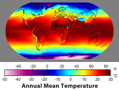
Next, let us note that the above picture represents average climate conditions, that is, averaged over the entire Earth's surface, and averaged over time. However, in reality, the incoming distribution of radiation varies in both space and time. We measure the radiation in terms of power (energy per unit time) per unit area, a quantity we term intensity or energy flux, which can be measured in watts per square meter (W/m2).
The dominant spatial variation occurs with latitude. On average, there is roughly 343 W/m2 of incoming shortwave solar radiation that is incident on the Earth, averaged over time, and over the Earth surface area. Obviously, there is more incoming solar radiation arriving at the surface near the equator than near the poles. On average, roughly 30%, or about 100 W/m2 of this incident radiation is reflected out to space by clouds and reflective surfaces of the Earth, such as ice and desert sand, leaving roughly 70% of the incoming solar radiation to be absorbed by the Earth's surface. The portion that is reflected by clouds and by the surface also varies substantially with latitude, owing to the latitudinal variations in cloud and ice cover:
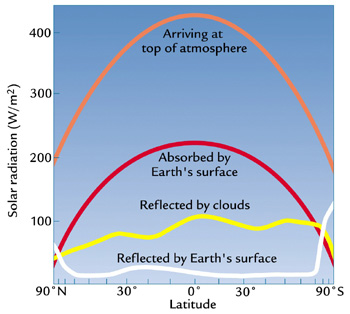
| Radiation (W/m 2) | 90ºn | 0º | 90ºs |
|---|---|---|---|
| ARRIVING AT THE TOP OF THE EARTH'S ATMOSPHERE | 200 | 420 | 190 |
| ABSORBED BYEARTH'S SURFACE | 95 | 210 | 93 |
| RELECTED BY cLOUDS | 95 | 100 | 95 |
| REFLECTED BY THE EARTH'S SURFACE | 97 | 91 | 110 |
Moreover, the distribution of outgoing longwave radiation also varies substantially with latitude:
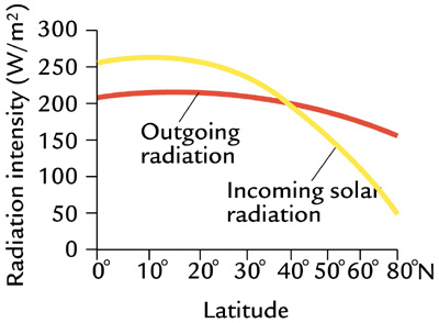
More terrestrial radiation is emitted from the warmer tropical regions and less emitted from the cold polar regions:
The disparity shown above (Figure 1.8) between the incoming solar radiation that is absorbed at the surface and the outgoing terrestrial radiation emitted from the surface poses a conundrum. As we can see in Figure 1.8, outgoing radiation exceeds incoming radiation near the poles, i.e., there is a deficit of radiation at the surface. Conversely, there is a surplus of incoming radiation near the equator. Should the poles, therefore, continue to cool down and the tropics continue to warm up over time?
Think About It!
Any idea what the solution to this conundrum might be?
Click for answer.
We will explore the details of how this is accomplished a bit later...
It is also worth noting that the incoming solar radiation is not constant in time. As we will see in later lessons, the output of the Sun, the so-called solar constant, can vary by small amounts on timescales of decades and longer. During the Earth's early evolution, billions of year ago, the Sun was probably about 30% less bright than it is today--indeed, explaining how the Earth's climate could have been warm enough to support life back then remains somewhat of a challenge, known as the "Faint Young Sun" paradox, although our understanding of it is improving.
Even more dramatic changes in solar insolation take place on shorter timescales—the diurnal and annual timescale. These changes, however, do not have to do with the net output of the Sun, but rather the distribution of solar insolation over the Earth's surface. This distribution is influenced by the Earth's daily rotation about its axis, which of course leads to night and day, and the annual orbit of the Earth about the Sun, which leads to our seasons. While there is a small component of the seasonality associated with changes in the Earth-Sun distance during the course of the Earth's annual orbit about the Sun (because of the slightly elliptical nature of the orbit), the primary reason for the seasons is the tilt of Earth's rotation axis relative to the plane defined by the Earth and the Sun, which causes the Northern Hemisphere and Southern Hemisphere to be preferentially oriented either towards or away from the Sun, depending on the time of year.
Check it out for yourself with this animation (1:49):
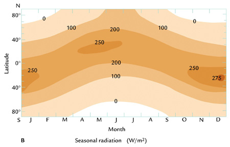
The consequence of all of this, is that amount of shortwave radiation received from the Sun at the top of the Earth's atmosphere varies as a function of both time of day and season:
Subtle changes in the Earth's orbital geometry (i.e., changes in the tilt of the axis, the degree of ellipticality of the orbit, and the slow precession of the orbit) are responsible for the coming and going of the ice ages over tens of thousands of years. We will revisit this topic later in the course.
Overview of the Climate System (part 3)
Atmospheric Circulation
We have seen above that the distribution of solar insolation over the Earth's surface changes over the course of the seasons, with the Sun, in a relative sense, migrating south and then north of the equator over the course of the year—that annual migration, between 23°S and 23°N, defines the region we call the tropics. As the heating by the Sun migrates south and north within the tropics over the course of the year, so does the tendency for rising atmospheric motion. As we have seen, warmer air is less dense than cold air, and where the Sun is heating the surface there is a tendency for convective instability, i.e., the unstable situation of having relatively light air underlying relatively heavy air. Where that instability exists, there is a tendency for rising motion in the atmosphere, as the warm air seeks to rise above the colder air. As a result, there is a tendency for rising air (and with it, rainfall) in a zone of low surface pressure known as the Intertropical Convergence Zone or ITCZ, which is centered roughly at the equator, but shifts north and south with the migration of the Sun about the equator over the course of the year. Due to the greater thermal inertia of the oceans relative to the land surface, the response to the shifting solar heating is more sluggish over the ocean, and the ITCZ shows less of a latitudinal shift with the seasons. By contrast, over the largest land masses (e.g., Asia), the seasonal shifts can be quite pronounced, resulting in dramatics shifts in wind and rainfall patterns such as the Indian monsoon.
The air rising in the tropics then sinks in the subtropics, forming a subtropical band of high surface pressure and low precipitation associated with the prevailing belt of deserts in the subtropics of both hemispheres. The resulting pattern of circulation of the atmosphere is known as the Hadley Cell circulation. In sub-polar latitudes, there is another region of low surface pressure, associated again with rising atmospheric motion and rainfall. This region is known as the polar front. These belts of high and low atmospheric surface pressure, and the associated patterns of atmospheric circulation also shift south and north over the course of the year in response to the heating by the Sun. You can explore the atmospheric patterns using the following animation (1:04):
The animation shows Hadley cells profile, ITCZ, pressure, and precipitation as they vary across a year.
Center of the Hadley cells (ITCZ) sit at 0 degrees in February and October. The cells move 10 to 15 degrees north February through June and then more 10 to 15 degrees south July through December. At any one point ITCZ varies depending on location around the globe.
Pressure has high and low pressure zones. Low pressure sits just north of the Arctic Circle, around the tropic of cancer and Greenland. High pressure sits above the Tropic of Cancer and along the Tropic of Capricorn. January through July most pressure zones south of the tropic of cancer grow while others shrink. July through December most pressure zones north of the Tropic of Capricorn grow and any south shrink. Two exceptions sit along the west coast of North and South America. They are both high-pressure zones and do the opposite of the other zones in their hemisphere.
Precipitation increases in the summer of each hemisphere and decreases in each hemispheres winter.
We have seen above that there is an imbalance between the absorbed incoming short wave solar radiation and the emitted outgoing long wave terrestrial radiation, with a relative surplus within the tropics and a relative deficit near the poles. We, furthermore, noted that the atmosphere and ocean somehow relieve this imbalance by transporting heat laterally, through a process known as heat advection. We are now going to look more closely at how the atmosphere accomplishes this transport of heat. We have already seen one important ingredient, namely the Hadley Cell circulation, which has the net effect of transporting heat poleward from where there is a surplus to where there is a deficit.
Wind patterns in the extratropics also serve to transport heat poleward. The lateral wind patterns are primarily governed by a balance between the previously discussed pressure gradient force (acting in this case laterally rather than vertically), and the Coriolis force, an effective force that exists due to the fact that the Earth is itself rotating. This balance is known as the geostrophic balance.
The Coriolis force acts at right angles to the direction of motion: 90 degrees to the right in the Northern Hemisphere and 90 degrees to the left in the Southern Hemisphere. The pressure gradient force is directed from regions of high surface pressure to regions of low surface pressure. As a consequence, geostrophic balance leads to winds in the mid-latitudes, between the subtropical high pressure belt and the sub-polar low pressure belt of the polar front, blowing from west to east. We call these westerly winds. For reasons that have to do with the vertical thermal structure of the atmosphere, and the combined effect of the geostrophic horizontal force balance and hydrostatic vertical force balance in the atmosphere, the westerly winds become stronger aloft, leading to the intense regions of high wind known as the jet streams in the mid-latitude upper troposphere.
Conversely, winds in the tropics tend to blow from east to west. These are known as easterly winds or, by the perhaps more familiar term, the trade winds. In the Northern Hemisphere, geostrophic balance implies counter-clockwise rotation of winds about low pressure centers and clockwise rotation of winds about high pressure centers. The directions are opposite in the Southern Hemisphere.
Due to the effect of friction at the Earth's surface, there is an additional component to the winds which blows out from high pressure centers and in towards low pressure centers. The result is spiraling in (convergence) towards low pressure centers and a spiraling out (divergence) about high pressure centers. The convergence of the winds toward the low pressure centers is associated with the rising atmospheric motion that occurs within regions of low surface pressure. The divergence of the winds away from the high pressure centers is associated with the sinking atmospheric motion that occurs within regions of high atmospheric pressure.
The inward spiraling low pressure systems in mid-latitudes constitute the polar front, which separates the coldest air masses near the poles from the warmer air masses in the subtropics. In fact, it is the unstable property of having clashing air masses with vastly different temperature characteristics, known as baroclinic instability, that is responsible for the existence of extratropical cyclones. The energy that drives the extratropical cyclones comes from the work done as surface air is lifted along frontal (i.e., cold front and warm front) boundaries. These extratropical storm systems relieve high-latitude deficit of radiation by mixing cold polar and warm subtropical air and, in so doing, transporting heat poleward, along the latitudinal temperature gradient.
You can explore the resulting large-scale pattern of circulation of the global atmosphere in the following animation (1:05):
Ocean Circulation (Gyres, Thermohaline Circulation)
While we have focused primarily on the atmosphere thus far, the oceans, too, play a key role in relieving the radiation imbalance by transporting heat from lower to higher latitudes. The oceans also play a key role in both climate variability and climate change, as we will see. There are two primary components of the ocean circulation. The first component is the horizontal circulation, characterized by wind-driven ocean gyres.
The major surface currents are associated with the ocean gyres. These include the warm poleward western boundary currents such as the Gulf Stream, which is associated with the North Atlantic Gyre, and the Kuroshio Current associated with the North Pacific Gyre. These gyres also contain cold equatorward eastern boundary currents such as the Canary Current in the eastern North Atlantic and the California Current in the western North Atlantic. Similar current systems are found in the Southern Hemisphere. The horizontal patterns of ocean circulation are driven by the alternating patterns of wind as a function of latitude, and, in particular, by the tendency for westerly winds in mid-latitudes and easterly winds in the tropics, discussed above.
An important additional mode of ocean circulation is the thermohaline circulation, which is sometimes referred to as the meridional overturning circulation or MOC. The circulation pattern is shown below:
By contrast with the horizontal gyre circulations, the MOC can be viewed as a vertical circulation pattern associated with a tendency for sinking motion in the high-latitudes of the North Atlantic, and rising motion more broadly in the tropics and subtropics of the Indian and Pacific Ocean. This circulation pattern is driven by contrasts in density, which are, in turn, largely due to variations in both temperature and salinity (hence the term thermohaline). The sinking motion is associated with relatively cold, salty surface waters of the sub-polar North Atlantic, and the rising motion with the relatively warm waters in the tropical and subtropical Pacific and Indian ocean.
The picture presented in Figure 1.11 above is a highly schematized and simplistic description of the actual vertical patterns of circulation in the ocean. Nonetheless, the conveyor belt is a useful mnemonic. The northward surface branch of this circulation pattern in the North Atlantic is sometimes erroneously called the Gulf Stream. The Gulf Stream, as discussed above, is part of the circulating waters of the wind-driven ocean gyre circulation. By contrast, the northward extension of the thermohaline circulation in the North Atlantic, is rightfully referred to as the North Atlantic Drift. This current system represents a net transport of warm surface waters to higher latitudes in the North Atlantic and is also an important means by which the climate system transports heat poleward from lower latitudes. Changes in this current system are speculated as having played a key role in past and potential future climate changes, as will be explored later in this course.
Other Fundamental Principles
Natural vs. Human Forcing

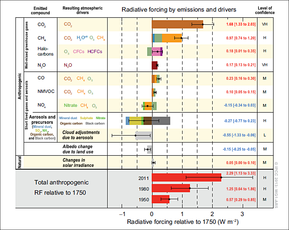
Let us consider more closely the above figure (Figure 1.12) from the IPCC Summary for Policy Makers . There is a lot of information packed in this figure. Figure 1.12 summarizes the relative impacts of various natural and human forcing factors on the Earth's climate. Later on in the course, we will look at how these forcing factors are likely to have impacted global mean temperature trends over the past century. In the meantime, we can make some rough assessment of the relative importance of the different factors as gauged by their estimated radiative forcing — measured by the energy per unit time that a given forcing factor exerts per square meter of the Earth's surface. The first thing to pay attention to is whether the indicated forcing factor is a warming factor (black dot to the right of zero) or cooling factor (black dot to the left of zero). The next thing to take note of is how high or low the forcing associated with that factor is, as indicated by the length of the bar. Finally, take note of the error bars (these are shown as the horizontal "barbell" symbols) indicating whether the factor in question is relatively well known, or relatively uncertain.
The forcings are separated into two fundamentally different categories: anthropogenic (that is, human-caused) and natural. You may be surprised to learn that while greenhouse gases are the primary anthropogenic forcing, there are other notable anthropogenic forcing contributions. Indeed, if one computes the net effect of anthropogenic aerosols (primarily sulfate) produced by industrial activity, adding together the direct and indirect effects of these aerosols, the total negative global radiative forcing (roughly -0.8 W/m2) is nearly half as large as the positive radiative forcing (roughly 1.7 W/m2) due to human-caused CO2 concentration increases (though the uncertainty associated with the most recent estimate of aerosol forcing is quite large). As we will see in later lectures, the cooling effect of these aerosols offset a substantial fraction of anthropogenic greenhouse warming over the past century.
One important historical natural forcing of climate is not shown in this diagram. This is the cooling effect of volcanic eruptions due to reflective aerosol injected into the stratosphere. Unlike other forcings, this volcanic forcing is episodic, rather than continuous in nature. Explosive volcanic eruptions may have a cooling effect on climate for several years. If there is a large number of eruptions over a sustained period of time, this can have an overall cooling impact on climate. We will revisit this issue in Lesson 4.
Feedback Mechanisms
The response of the climate to forcing, whether natural or human-caused, would be far more modest than it is, were it not for the influence of feedback mechanisms. Feedback mechanisms are mechanisms within the climate system that act to either attenuate (negative feedback) or amplify (positive feedback) the response to a given forcing. On balance, the feedbacks are believed to be positive in the sense that the response of the climate system to a positive forcing is greater than one would expect from the forcing alone, because of the net warming effect arising from these responses.
The principle feedback mechanisms, relevant to climate change on historical timescales, are:
- The water vapor feedback. Warming atmosphere can hold larger amounts of water vapor. Since water vapor is a greenhouse gas, this leads to further warming: a Positive Feedback
- The ice-albedo feedback. Surface of the Earth has less snow/ice as it warms, leading to less reflection and greater absorption of incoming solar radiation: a Positive Feedback
- The cloud radiative feedbacks. There are different competing effects:
- Warmer atmosphere produces more low clouds. The primary impact of more low clouds would be to reflect more solar radiation out to space: a Negative Feedback
- Warmer atmosphere produces more high clouds, like cirrus. The primary impact of such thin, high clouds is to increase the greenhouse effect due to their ability to trap much of the outgoing longwave terrestrial radiation while remaining largely transparent to incoming shortwave solar radiation: a Positive Feedback
On balance, it has been believed that the negative cloud radiative feedbacks win over the positive cloud radiative feedbacks - though the low cloud feedbacks are quite uncertain, and the overall cloud radiative feedback could very well be positive.
The net effect of all these feedbacks is positive and serves to increase the warming due a particular external forcing (be it increased greenhouse gas concentrations due to fossil fuel emissions, increased solar output, or some other external forcing) beyond what would be expected purely from that factor alone. For example, a doubling of CO2 concentrations relative to pre-industrial levels would, in the absence of feedbacks, lead to roughly 1.25°C warming. However, our best estimates indicate that the positive water vapor feedback would add about 2.5°C additional warming, while the positive ice albedo feedback adds about 0.6°C warming. While substantially more uncertain, the negative cloud radiative feedback could lead to just under 2°C cooling. Add up the numbers, and the total comes to about 2.5°C warming (actually, current generation climate models average closer to 3°C).
This quantity--how much we expect the Earth to warm once it equilibrates to a doubling of greenhouse gas concentrations--is known as the equilibrium climate sensitivity. We will explore this key concept in more detail in subsequent lectures.
The Carbon Cycle
The traditional concept of climate sensitivity envisions the concentration of CO2 and other greenhouse gases as specified (i.e., doubled from some initial level), and calculates the expected warming. This construction is somewhat artificial, however, because activities, such as fossil fuel burning, do not directly regulate the concentration of CO2 or other greenhouse gases, but instead govern the atmospheric emissions, which can interact with the climate system. For example, life on land and in the ocean can both take up and give off CO2: CO2 is taken up during photosynthesis — production of organic matter by green plants, and given off during respiration (or remineralization) — a reverse process during which organic matter is decomposed. As climate becomes warmer, the living organisms are affected by the change, e.g., green plants might consume more CO2 because the growing season becomes longer and the plants have more time for photosynthesis; or, on the other hand, warmer temperatures might induce bacterial activity and the rates of decay of organic matter, causing an increase in the CO2 emissions. In general, the Earth system processes of chemical, physical, or biological origin that emit CO2 to the atmosphere are referred to as carbon sources, while those that take up CO2 from the atmosphere are referred to as carbon sinks or losses. Climate change affects the characteristics of living things, as well as other components of the climate system, such as, for example, the overturning ocean circulation (which helps to sequester atmospheric carbon in the deep ocean), and therefore can influence various carbon sources and sinks that exist within the Earth system.
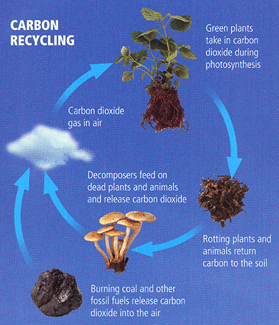
- Burning coal and other fossil fuels release carbon dioxide into the air
- Carbon dioxide gas in air
- Green plants take in carbon dioxide during photosynthesis
- Rotting plants and animals return carbon to the soil
- Decomposers feed on dead plants and animals and release carbon dioxide (Repeats/Return to step 1)
© 2015 Pearson Education, Inc.
We refer to the amount of emitted CO2 that actually stays in the atmosphere as the airborne fraction of CO2. So far, only roughly half of our carbon emissions remain airborne. The other half has been absorbed by carbon sinks. The primary carbon sink is the upper ocean, which has absorbed roughly 25-30% of the CO2, while the terrestrial biosphere has absorbed another 15-20% of the CO2.
These sinks are not constant over time, however. Numerous studies indicate that both the upper ocean and terrestrial biosphere are likely to become less able to absorb and hold additional CO2 as the globe warms. Were this to happen, the airborne fraction of CO2 in the atmosphere would increase, and CO2 would accumulate in the atmosphere more quickly for a given rate of emissions. Such responses are known as the carbon cycle feedbacks, because they have the ability to influence the accumulation of CO2 in the atmosphere.
The existence of carbon cycle feedbacks forces us to reconsider the concept of climate sensitivity discussed earlier. Consider for example, the accumulated carbon emissions that we might calculate would lead to a doubling of CO2 in the atmosphere in the absence of carbon cycle feedbacks. As the climate warms, the positive carbon cycle feedbacks discussed above would cause the airborne fraction to increase. As a result, the final increase in atmospheric CO2 would be greater than the originally calculated doubling. Accordingly, there would be even more warming than one would estimate from applying the standard concept of equilibrium climate sensitivity to the original estimated slug of carbon emissions.
Such complications lead to the more general notion of the Earth System sensitivity. We will revisit these concepts later in the course.
Lesson 1 Discussion
Activity
Directions
At this point, you have completed the Course Orientation and the first lesson for METEO 469. Let's talk! Please participate in an online discussion of the course in general and of the material we have covered thus far. Please share your thoughts about the general topic of this course and what you hope to learn. Also, please discuss the material presented in Lesson 1.
This discussion will take place in a threaded discussion forum in Canvas (see the Canvas Guides for the specific information on how to use this tool) over approximately a week-long period of time. Since the class participants will be posting to the discussion forum at various points in time during the week, you will need to check the forum frequently in order to fully participate. You can also subscribe to the discussion and receive e-mail alerts each time there is a new post.
Please realize that a discussion is a group effort, and make sure to participate early in order to give your classmates enough time to respond to your posts.
Post your comments addressing some aspect of the material that is of interest to you and respond to other postings by asking for clarification, asking a follow-up question, expanding on what has already been said, etc. For each new topic you are posting, please try to start a new discussion thread with a descriptive title, in order to make the conversation easier to follow.
Suggested topics
The purpose of the discussion is to facilitate a free exchange of thoughts and opinions among the students, and you are encouraged to discuss any topic within the general discussion theme that is of interest to you. If you find it helpful, you may also use the topics suggested below.
General discussion of METEO 469
- Why are you taking this course?
- Why are you interested in climate change?
- Is it important to you to understand the scientific basis of climate science?
- Is it important to you to learn about impacts of climate change?
- What do you hope to learn in this course?
Lesson 1: Introduction to Climate and Climate Change
- In your understanding, what is the difference between the climate and the weather? Why is it important to differentiate between the two?
- Discuss natural versus anthropogenic climate change.
- What are feedback mechanisms in regard to the climate system? Can we know all feedback mechanisms in our climate system? Which mechanisms are considered most important and why?
- Discuss the concept of climate sensitivity. Why is this concept useful?
- Discuss the components of the carbon cycle and how carbon sources and sinks influence atmospheric CO2 levels.
Submitting your work
- Go to Canvas.
- Go to the Home tab.
- Click on Lesson 1 discussion: General Discussion of METEO 469.
- Post your comments and responses.
Grading criteria
You will be graded on the quality of your participation. See the online discussion grading rubric for the specifics on how this assignment will be graded. Please note that you cannot get full credit on this assignment if you wait until the last day of the discussion to make your first post.
Lesson 1 Summary
We have reviewed the essential basic concepts necessary for understanding climate change and global warming, including:
- The concepts of climate, climate change, and global warming;
- The components of the Earth's climate system: the atmosphere, oceans, cryosphere, and biosphere;
- The structure and composition of the Earth's atmosphere;
- The concepts of radiation and energy balance;
- The nature of the circulation of the atmosphere and the oceans;
- The concept of radiative forcing;
- Climate feedbacks and climate sensitivity;
- Carbon cycle feedbacks and the Earth System sensitivity.
We are now well-equipped to begin digging into the details. Our first foray will be into the world of climate observations. What data are available that can inform our understanding of how climate has changed over historic time? What indirect data are available that place historical observation in a longer-term context? How do we analyze such data to assess whether there is indeed "climate change"? This will be our next topic.
Reminder - Complete all of the module tasks!
You have finished Lesson 1. Double-check the list of requirements on the first page of this lesson to make sure you have completed all of the activities listed there before beginning the next lesson.