'SRES' Scenarios and 'RCP' Pathways

Scientists attempt to create scenarios of future human activity that represent plausible future greenhouse emissions pathways. Ideally, these scenarios span the range of possible future emissions pathways, so that they can be used as a basis for exploring a realistic set of future projections of climate change.

In the early IPCC assessments, the most widely used and referred-to family of emissions scenarios were the so-called SRES scenarios (for Special Report on Emissions Scenarios) that helped form the basis for the IPCC Fourth Assessment Report. These scenarios made varying assumptions ('storylines') regarding future global population growth, technological development, globalization, and societal values. One (the A1 'one global family' storyline chosen by Michael Mann and Lee Kump in version 1 of Dire Predictions) assumed a future of globalization and rapid economic and technological growth, including fossil fuel intensive (A1FI), non-fossil fuel intensive (A1T), and balanced (A1B) versions. Another (A2, 'a divided world') assumed a greater emphasis on national identities. The B1 and B2 scenarios assumed more sustainable practices ('utopia'), with more global-focus and regional-focus, respectively.

Let us now directly compare the various SRES scenarios both in terms of their annual rates of carbon emissions, measured in gigatons (Gt) of carbon (1Gt = 10¹² tons), and the resulting trajectories of atmospheric ${\text{CO}}_{\text{2}}$ concentrations. Getting the concentrations actually requires an intermediate step involving the use of a simple model of ocean carbon uptake, to account for the effect of oceanic absorption of atmospheric ${\text{CO}}_{\text{2}}$.

Figure 6.1: Estimated ${\text{CO}}_{\text{2}}$ concentrations (top) and Annual Carbon Emissions (bottom) for the Various IPCC SRES Scenarios.

Credit: Robert A. Rohde / Global Warming Art

We can see from the above comparison how various trajectories of our future carbon emissions translate to atmospheric ${\text{CO}}_{\text{2}}$ concentration trajectories. From the point of view of controlling future ${\text{CO}}_{\text{2}}$ concentrations, these graphics can be quite daunting. Depending on the path chosen by society, we could plausibly approach ${\text{CO}}_{\text{2}}$ concentrations that are quadruple pre-industrial levels by 2100. Even in the best case of the SRES scenarios, B1, we will likely reach twice pre-industrial levels (i.e., around 550 ppm) by 2100. And to keep ${\text{CO}}_{\text{2}}$ concentrations below this level, we can see that we have to bring emissions to a peak by 2040, and ramp them down to less than half current levels by 2100.

You might wonder what scenario do we actually appear to be following? Over the first ten years of these scenarios, observed emissions actually were close to the most carbon intensive of the SRES scenarios—A1FI. This gives you an idea of how challenging the problem of stabilizing carbon emissions at levels lower than twice pre-industrial actually is.

Figure 6.2: Observed Historic Emissions Compares with the Various IPCC SRES Scenarios.

Credit: The Copenhagen Diagnosis

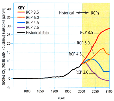
One problem with the SRES scenarios—indeed, a fair criticism of them—is that they do not explicitly incorporate carbon emissions controls. While some of the scenarios involve storylines that embrace generic notions of sustainability and environmental protection, the scenarios do not envision explicit attempts to stabilize ${\text{CO}}_{\text{2}}$ concentrations at any particular level. For the Fifth Assessment Report, a new set of scenarios, called Representative Concentration Pathways (RCPs), was developed. They are referred to as pathways to emphasize that they are not definitive, but are instead internally consistent time-dependent forcing projections that could potentially be realized with multiple socioeconomic scenarios. In particular, they can take into account climate change mitigation policies to limit emissions. The scenarios are named after the approximate radiative forcing relative to the pre-industrial period achieved either in the year 2100, or at stabilization after 2100. They were created with 'integrated assessment models' that include climate, economic, land use, demographic, and energy-usage effects, whose greenhouse gas concentrations were then converted to an emission's trajectory using carbon cycle models.

The RCP2.6 scenario peaks at 3.0 W / m² before declining to 2.6 W / m² in 2100, and requires strong mitigation of greenhouse gas concentrations in the 21^st century. The RCP4.5 and RCP6.0 scenarios stabilize after 2100 at 4.2 W / m² and 6.0 W / m², respectively. The RCP4.5 and SRES B1 scenarios are comparable; RCP6.0 lies between the SRES B1 and A1B scenarios. The RCP8.5 scenario is the closest to a ‘business as usual’ scenario of fossil fuel use, and has comparable forcing to SRES A2 by 2100.

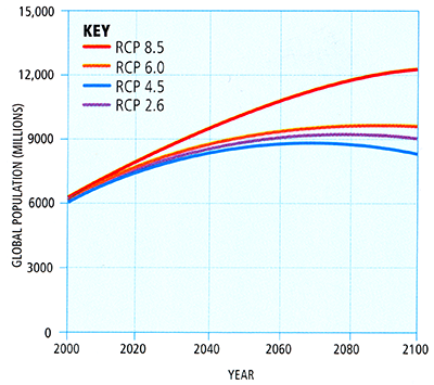
In all RCPs global population levels off or starts to decline by 2100, with a peak value of 12 billion in RCP8.5. Gross domestic product (GDP) increases in all cases; of note, the RCP2.6 pathway has the highest GDP, though it has the least dependence on fossil fuel sources. Carbon dioxide emissions for all RCPs except the RCP8.5 scenario peak by 2100.

Even the RCPs have encountered a fair bit of criticism.  For the recently released Sixth IPCC Assessment Report, scientists and modelers are using Shared Socioeconomic Pathways (SSPs), which link specific policy decisions with projected emissions outcomes.  The readings this week include a Commentary from the journal Nature about the issue of RCPs and the path forward with SSPs.

Figure 6.3a: RCP Global Population Scenarios

Click here for text description of Figure 6.3a

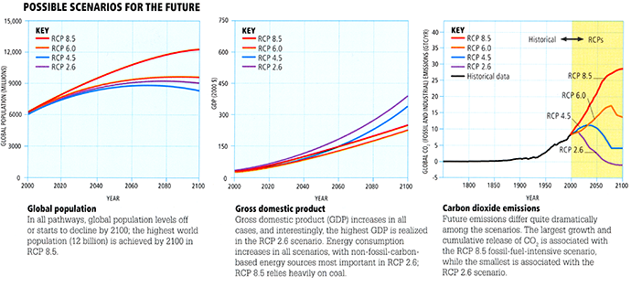
Global Population

In all pathways, global population levels off or starts to decline by 2100; the highest world population (12 billion) is achieved by 2100 in RCP 8.5

Gross Domestic Product

Gross Domestic product (GDP) increases in all cases, and interestingly, the highest GDP is realized in the RCP 2.6 scenario. Energy consumption increases in all scenarios, with non-fossil-carbon-based energy sources most important in RCP 2.6; RCP 8.5 relies heavily on coal

Carbon Dioxide Emissions

Future emissions differ quite dramatically among the scenarios. The largest growth and cumulative release of CO₂ is associated with the RCAP 8.5 fossil-fuel-intensive scenario, while the smallest is associated with the RCP 2.6 scenario

Credit: Mann & Kump, Dire Predictions: Understanding Climate Change, 2^nd Edition
© 2015 Dorling Kindersley Limited.

Figure 6.3b: RCP Global Population Scenarios

Credit: Mann & Kump, Dire Predictions: Understanding Climate Change, 2^nd Edition
© 2015 Dorling Kindersley Limited.

Figure 6.4: RCP Gross Domestic Product Scenarios.

Credit: Mann & Kump, Dire Predictions: Understanding Climate Change, 2^nd Edition
© 2015 Dorling Kindersley Limited.

Figure 6.5: RCP Carbon Dioxide Emission Scenarios.

Credit: Mann & Kump, Dire Predictions: Understanding Climate Change, 2^nd Edition
© 2015 Dorling Kindersley Limited.

With all of these scenarios, stabilizing CO₂ concentrations requires not just preventing the increase of emissions, but reducing emissions. This leads naturally to our next topic—the topic of stabilization scenarios.