Stabilizing CO2 Concentrations

Before we proceed, it is useful to cover a few more important details. You may recall from an earlier lesson that the radiative forcing due to a given increase in atmospheric ${\text{CO}}_{\text{2}}$ concentration, $\Delta F_{C{O}_2}$ , can be approximated as:

$$\Delta F_{C{O}_2}=5.35\ln \left(\frac{\left[C{O}_2\right]}{{\left[C{O}_2\right]}_0}\right)$$

where ${\left[C{O}_2\right]}_0$ is the initial concentration and $\left[C{O}_2\right]$ is the final concentration. This gives a forcing for doubling of ${\text{CO}}_{\text{2}}$ from pre-industrial values (i.e., ${\left[C{O}_2\right]}_0$ = 280 ppm and $\left[C{O}_2\right]$ = 560 ppm) of just under $\mathrm{4 }W{m}^{-2}$. Given the typical estimate of climate sensitivity we discussed during the past two lessons, we know that this forcing translates to about 3°C warming. That means, we get about 0.75°C warming for each $W{m}^{-2}$ of radiative forcing.

If you successfully answered the question above, you know that the ${\text{CO}}_{\text{2}}$ increases so far should have given rise to 1.5°C warming of the globe. Yet we have only seen about 1.0°C warming. Are the theoretical formulas wrong? Did we make a mistake? Actually, it is neither. First of all, we know that it takes decades for the climate system to equilibrate to a rise in atmospheric ${\text{CO}}_{\text{2}}$, so we have not yet realized the expected equilibrium warming indicated by the equilibrium climate sensitivity. Models indicate that there is as much as another 0.5°C of warming still in the pipeline, due to the ${\text{CO}}_{\text{2}}$ increases that have taken place already. That alone would almost explain the 0.7°C discrepancy between the warming we expect, and the lesser warming we've observed.

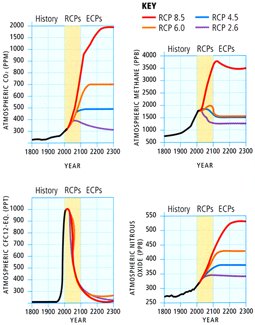
However, we have forgotten two other things that—as it happens—roughly cancel out! First of all, ${\text{CO}}_{\text{2}}$ is not the only greenhouse gas whose concentrations we have been increasing through industrial and other human activities. There are other greenhouse gases—methane, nitrous oxide, and others—whose concentrations we have increased, and whose concentrations are projected to continue to rise in the various SRES and RCP scenarios we have examined.

Figure 6.6: Greenhouse Gas Levels Resulting from Various Emissions Scenarios.

Credit: Mann & Kump, Dire Predictions: Understanding Climate Change, 2^nd Edition
© 2015 Dorling Kindersley Limited.

We need to account for the effect of all of these other greenhouse gases. We can do this using the concept of ${\text{CO}}_{\text{2}}$ equivalent (${\text{CO}}_{\text{2}}$_eq). ${\text{CO}}_{\text{2}}$_eq is the concentration of ${\text{CO}}_{\text{2}}$ that would be equivalent, in terms of the total radiative forcing, to a combination of all the other greenhouse gases. If we take into account the rises in methane and other anthropogenic greenhouse gases, then the net radiative forcing is equivalent to having increased ${\text{CO}}_{\text{2}}$ to a substantially higher, roughly 485 ppm! In other words, the current value of ${\text{CO}}_{\text{2}}$_eq is 485 ppm. This fact has caused quite a bit of confusion, leading some commentators (see this RealClimate article) to incorrectly sound the alarm that it is already too late to stabilize ${\text{CO}}_{\text{2}}$ concentrations at 450 ppm and, hence, to avoid breaching the targets that have been set by some as constituting dangerous anthropogenic interference with the climate (see this article by Michael Mann for a discussion of these considerations).

Nonetheless, if ${\text{CO}}_{\text{2}}$_eq has reached 485ppm, does that mean that we are committed to the net warming that can be expected from a concentration of 485 ppm ${\text{CO}}_{\text{2}}$? Well, yes and no. The other thing we have left out is that greenhouse gases are not the only significant anthropogenic impact on the climate. We know that the production of sulfate and other aerosols has played an important role, cooling substantial regions of the Northern Hemisphere continents, in particular, during the past century. The best estimate of the impact of this anthropogenic forcing, while quite uncertain, is roughly -0.8 $W/m^2$ of forcing, which is equivalent—in this context—to the contribution of negative 60 ppm of ${\text{CO}}_{\text{2}}$. If we add -60 ppm to 485 ppm we get 425 ppm—which is closer to the current actual ${\text{CO}}_{\text{2}}$ concentration of 408 ppm. So, in other words, if we take into account not only the effect of all other greenhouse gases, but also the offsetting cooling effect of anthropogenic aerosols, we end up roughly where we started off, considering only the effect of increasing atmospheric ${\text{CO}}_{\text{2}}$ concentration through fossil fuel burning.

It is, therefore, a useful simplification to simply look at atmospheric ${\text{CO}}_{\text{2}}$ alone as a proxy for the total anthropogenic forcing of the climate, but there are some important caveats to keep in mind:

(1) the various scenarios assume that the sulfate aerosol burden remains unchanged. If we instead choose to clean up the atmosphere to the point of scrubbing all current sulfate aerosols from industrial emissions, we are left with the faustian bargain of experiencing the additional climate change impacts of a sudden effective increase of atmospheric ${\text{CO}}_{\text{2}}$ of 60 ppm;

(2) not all greenhouse gases are created the same—some, such as methane, have far shorter residence times in the atmosphere (timescale of years) than does ${\text{CO}}_{\text{2}}$, which persists for centuries.

That means that there is a far greater future climate change commitment embodied in a scenario of pure ${\text{CO}}_{\text{2}}$ emissions than the same ${\text{CO}}_{\text{2}}$ equivalent emissions consisting largely of methane. This has implications for the abatement strategies we will discuss later in the course.

These limitations notwithstanding, let us now consider the impact of various pure ${\text{CO}}_{\text{2}}$ scenarios. Let us focus specifically on scenarios that will stabilize atmospheric ${\text{CO}}_{\text{2}}$ at some particular level, i.e., so-called stabilization scenarios. Invariably, these scenarios involve bringing annual emissions to a peak at some point during the 21st century, and decreasing them subsequently. Obviously, the higher we allow the concentrations to increase and the later the peak, the higher the ultimate ${\text{CO}}_{\text{2}}$ concentration is going to be. The various possible such scenarios are shown below in increments of 50 ppm. If we are to stabilize ${\text{CO}}_{\text{2}}$ concentrations at 550 ppm, we can see that ${\text{CO}}_{\text{2}}$ emissions should be brought to a peak of no more than 8.7 gigatons of carbon per year, by around 2050, and reduced below 1990 levels (i.e., 6 gigatons of carbon per year) by 2100. For comparison, as we saw earlier that current emissions are at roughly 8.5 gigatons per year and rising at the rate of the carbon-intensive A1FI SRES emissions scenario, so we are already "behind the curve" so to speak, even for 550 ppm stabilization.

For 450 ppm stabilization, the challenge is far greater. According to the figure below, we would have had to bring emissions to a peak before 2010 at roughly 7.5 gigatons per year, and lower them to roughly 4 gigatons per year (i.e., 33% below 1990 levels) by 2050. Obviously, that train has already left the station. Alternatively, the RCP2.6 pathway is an example of a 450 ppm stabilization scenario consistent with where we are now, that involves bringing emissions to a peak within the next decade below 10 gigatons per year, and reducing them far more dramatically, to near zero 80% by 2100 through various mitigation policies. With every year, we continue with business-as-usual carbon emissions, achieving a 450 ppm stabilization target becomes that much more difficult, and involves far greater reduction of emissions in future decades. It is for this reason that the problem of greenhouse gas stabilization has been referred to by some scientists as a problem with a very large procrastination penalty.

Figure 6.7: Annual ${\text{CO}}_{\text{2}}$ emissions and Resulting ${\text{CO}}_{\text{2}}$ concentrations for Various Stabilization Scenarios.

Credit: Robert A. Rohde / Global Warming Art