Lesson 6. Reanalysis Data Sets
Motivate...
During your exploration of weather and climate data, you might have encountered data sets either in "NetCDF" (pronounced "net C-D-F") or "GRIB" (sounds like "rib") formats. If so, you can be assured that you have left the realm of the casual data user and have entered the domain of the true data scientist. These file types were created to have a machine-independent way to store and transport vast arrays of meteorological or geophysical data. The GRIB (or GRidded Binary) data standard was developed by the WMO and is the most basic format of gridded meteorological data, from satellite images to model data. NetCDF, on the other hand, is what I would describe as a high-level data standard that was developed by Unidata [1] (a consortium of research and educational partners). NetCDF files are highly versatile, are also machine independent, and (more importantly) are self-describing, which means that all the information you need to know about the data is packaged right along with the data itself.
I'll provide links with more details on these file standards later in the lesson. However, before you dive in, let me point out some important points to keep in mind. First, both file types are binary files. That means that they are only readable by a computer (you can't just open the files and expect to see numbers). This means that you must have a special set of library functions and/or programs to read both NetCDF and GRIB files (remember that these files are meant for the scientists, not the casual consumer). These libraries and programs are machine dependent and can be a real pain to install on your particular system, which is particularly the case if you are not running a Linux system (data scientists must all run Linux systems). We'll need to overcome some technological challenges in order to develop a workflow that suits our needs. However, there are tools out there if you look around. Hopefully, with the programs that I point you to, you'll be able to perform most (if not all) of the analyses you need.
If I had to identify a significant difference between NetCDF and GRIB files, it would be in how the data are stored and accessed in each. GRIB files are simply a series of sequential records packed into a single file. Each record represents a grid of a single variable at a single time (like pages in an atlas). Each page has a description at the top (called the "header") describing the grid... what it is, how big, what the numbers are, etc. Grids can be extracted from the file and displayed/processed using the information in the header, but you are limited to extracting only an entire record at a time. Extracting a value at a particular latitude/longitude (for example) requires much more work because, for the sake of file size, that information is not stored with the actual data. If this seems annoying, I agree... it is. But remember that GRIB format files are simply containers for large data sets likely processed automatically by some heavy-duty computer power. That's not to say we can't do likewise, but know that if you need GRIB data of any kind, you'd better need a lot of it to make up for the time you will spend writing the scripts needed to process the data.
The good news is that NetCDF files are much more friendly. They are still in binary format, however, and you will need the proper set of tools to read them. The thing that makes NetCDF files better than their GRIB cousins are that NetCDF files are totally self-contained. That is, they have ALL the information you would need to know about the data included within their description section. This includes variable dimensions/units, a time-base definition, and the specific data structure within the file. What's more, NetCDF files are not sequential records of 2D data. Unlike the single book analogy where the data are stored on individual pages, NetCDF files represent a hypercube (more than 3 dimensions) of data that you may interact with in any way you wish. For example, in a NetCDF file, you might have model temperatures over a 3D domain (latitude, longitude, height) AND in time. In this 4-dimensional configuration, you might retrieve a horizontal grid, a vertical slice, a profile, or a time-series at a particular point in space -- all with relative ease. These are pretty amazing files and I think once you get the hang of it, you are going to wish everything was in NetCDF format.
So, in this lesson, we are going to start off by working with the NetCDF file structure, then move on to GRIB. Along the way you'll also be introduced to two new data sources: model reanalyses (specifically the North American Regional Reanalysis) and the National Digital Forecast Database. This will give you even more choices when it comes to finding data that will suit your needs.
Read on!
What is NetCDF?
Prioritize...
After completing this section, you will have the NetCDF files installed on your computer.
Read...
If you're not familiar with NetCDF files, please read the following sections/links before installing the libraries:
NetCDF Reading Assignment
- For an overview, start with the Wikipedia page [2].
- Next, read the "What Is NetCDF" section of the NetCDF FAQ [3].
- Finally, read the first four sections of the NetCDF User's Guide [4]. Make sure that you understand the various parts of a NetCDF file (and what they are used for).
Now that you know more about NetCDF files, it's time to install the libraries which are operating-system dependent. Depending on your level of technical skill you can get pre-built libraries or build them yourself from the source code. I just grabbed the pre-built Windows version of NetCDF-4 (64-bit) [5]. If you are a MAC user, you will want to use a package manager called Homebrew [6]or MacPorts [7]to facilitate the install. Here is a set of instructions [8] using MacPorts that you might find helpful (searching "netcdf library homebrew" will provide useful pages for that manager). There are instructions for LINUX users [9] as well, but you guys are likely well-versed in performing such installs.
It is absolutely imperative that you get the NetCDF libraries installed correctly! You won't be able to proceed without them. To verify your install, you should be able to type "ncdump" at any command prompt and see a set of usage instructions (and no errors). Please contact me ASAP if you are having trouble. In the next section, we will link up the NetCDF libraries with the R interface.
Read on after you've completed this step.
NetCDF, the NARR, and R
Prioritize...
In this section, you will link the NetCDF libraries with R through the package "ncdf4". You will also retrieve a file from the North American Regional Reanalysis to test the R/NetCDF interface.
Read...
The first thing that we want to do is install the ncdf4 package which is a set of function calls that connect R to the NetCDF libraries that you installed. This will allow us to read NetCDF files directly into R and perform all the graphing and analysis that we have done with other sources of data.
Do you remember how to install a package in R-Studio? When you are finished, you should be able to type the command: nc_version() at the R-prompt and be answered back with the version of the installed library. If you don't remember, I have placed the commands below (click to reveal).
> install.packages("ncdf4")
> library(ncdf4)
Now that we have the ncdf4 library installed, let's get some data. There are many sources of geophysical data in NetCDF format. However, we are going to be looking at data from the North American Regional Reanalysis (NARR, pronounced like "car").
To understand how a model reanalysis is created, recall that a traditional numerical model is "initialized" by mapping various point and spatial observations onto a defined grid (a process called "data assimilation"). The numerical model then applies mathematical equations to advance the model forecast variables in time. As time goes on, however, errors grow within these predicted fields so that eventually they are useless as predictors. A model reanalysis differs from a prognostic model in that it uses historical data for its initialization. This means that at regular time periods, more observations can be added to the model to "correct" (or nudge) the predicted fields. This technique doesn't eliminate error altogether, but it gives you a long-term, continuous (in time and space) record of data for vast numbers of observed and calculated variables. If used properly, reanalysis data can prove an invaluable input stream to weather and climate analytics decisions.
Before proceeding further, read these two articles on model reanalysis...
NARR Reading Assignment
- For an overview, start with the Wikipedia page. [10]
- Next, read this paper on the NARR [11] published in the Bulletin of the American Meteorological Society.
- Finally, go to the ESRL/PSD NARR homepage [12] and browse the information/links provided. Note that there are some handy plotting pages that will allow you to get quick graphics of NARR output.
If you go looking for NARR data, you will find the raw source to be Research Data Archive (RDA) at the National Centers for Atmospheric Research (NCAR) [13]. Here all of the NARR data is housed, from 1979 to present day. The problem with this site is that all of the raw data are stored in huge (~1 GB) files in GRIB format. This means that we will need to do considerable work to dig out the variables that we might want to analyze. We'll get to that problem later in the lesson. For now, let's return to the ESRL/PSD NARR homepage [14] where the NARR files have been segmented and converted to NetCDF format. Yay!
Your next goal is to select a NARR output file (in NetCDF format) and save it to your local hard drive. Notice on the page that NARR data is separated into three categories: pressure-level data, subsurface data, and mono-level data. We are interested in the mono-level data because we want surface temperatures (mono-level data is any surface in the model that is not defined by a constant pressure level). Clicking on the mono-level link takes you to a page with a huge table [15] which lists all of the available variables. Find the variable for 3-hour temperature and click on the download file prefix (should be "air.sfc.yyyy.nc"). This will take you to a folder containing all of the yearly files. Grab one of your choosing (scroll down) and save it to your local drive (I chose 1988). To check that everything worked correctly, you can open a command prompt in the folder you saved the file and type: ncdump -h air.sfc.1988.nc (or whatever your file is named) and see a description of the file header (the different variables and dimensions that describe the data).
Now we are ready to dig into the data! Read on.
Plotting NARR data
Prioritize...
After completing this section, you will have successfully installed the "ncdf4" library in R and retrieved data from a NetCDF file.
Read...
At this point, you have installed the NetCDF libraries, the ncdf4 R-library, and you have a data file. Let's crack it open... (at this point, you should be familiar with what we are doing in R). Start a new R-script file, enter the code below, and save it in the same directory as your data file (for simplicity's sake). By the way, don't forget to set your working directory to that of the source file.
# if for some reason we need to reinstall the
# package, then do so.

if (!require("ncdf4")) {
  install.packages("ncdf4") }

# include the NetCDF library
library(ncdf4)

# We'll also need these libraries for plotting maps of data
library(fields)
library(maps)

# open the NetCDF file
nc <- nc_open("air.sfc.1988.nc")
Source this code and then type "nc" at the R command prompt. You should see a description of the file contents. Notice that it contains 4 variables (3 actually, if we ignore the map projection information) and 3 dimensions (x, y, and time). You can also see that latitude and longitude are a function of x and y, while the temperature variable ("air") is a function of space (x and y) as well as time. We can extract the total size of the "air" variable by typing the command: nc$var$air$varsize at the command prompt (notice that the variable information is stored in a complex data frame called nc$var). The values for each dimension can be obtained by querying the $dims data frame: nc$dim$time$vals. If you do so, you'll notice that the times are in some strange integer format. If we go back to the file definitions (typing nc or specifically nc$dim$time$units) we see that the time base is "hours since 1800-01-01 00:00:00". Therefore, we need to do a bit of manipulation to have times that make some sense. Fortunately, R comes to the rescue...
# First get the time data in hours
ncdates = nc$dim$time$vals  #hours since 1800-1-1

# Next set a date/time object at the start of the time base
origin = as.POSIXct('1800-01-01 00:00:00', tz = 'UTC')

# Now convert the time string to seconds and add it to the origin.
# ncdates should be a series of dates and times which matches the
# file you chose.
ncdates = origin + ncdates*(60*60)

# Let's pick a date/time we want to plot
# This should actually go at the top of your code
target_datetime<-"1988-05-04 12:00 UTC"

# Find the index of the time entry that matches the target
time_index=which(ncdates==as.POSIXct(target_datetime, tz='UTC'))
Now that we have time sorted out, what about the latitude and longitude? If you haven't already, notice that NetCDF files are not like serialized text files. By that, I mean that there are no entries like: "lat1, long1, temp1". That would be an unnecessary repetition of the variables "lat" and "lon" for each grid of temperature. Instead, latitude and longitude are defined by their own grid which is equal in size to the temperature grids. You might also have noted that latitude and longitude are variables, not dimensions. The dimensions "x" and "y" define the data space and latitude/longitude are mapped onto each (x,y) pair. This is because latitude and longitude are not equally spaced, due to the map projection (Lambert conformal). So, if we are going to plot a grid of temperature versus (latitude/longitude), we need to compute arrays for those variables as well.
# How big is the dataset?
# Note: the "$air" portion must match your variable name
data_dims<-nc$var$air$varsize

#Get the lats/lons using ncvar_get
lats=ncvar_get(nc, varid = 'lat',
               start = c(1,1),
               count = c(data_dims[1],data_dims[2]))

lons=ncvar_get(nc, varid = 'lon',
               start = c(1,1),
               count = c(data_dims[1],data_dims[2]))

# The longitude values are not compatible with my map
# plotting function, so I need to fix this.
lons<-ifelse(lons>0,lons-360,lons)
Let's look at the function ncvar_get(). Notice that for the retrieval of lat/lon we need to know how many values to get in each dimension. I could hard-code this, but why not just query the file to get the dimensions (that's the advantage of the self-describing nature of NetCDF). The "get" function takes a pointer to the file, the variable ID, a starting point and a counter in each dimension. Since we want the entire grid, we'll start at (1,1) and retrieve the max value for each dimension. Now, let's get the temperature data...
# Because we are retrieving a multi-dimensional array, we must
# set aside some space beforehand.
temp_out = array(data = NA, dim = c(data_dims[1],data_dims[2],1))

# get the temperature data (notice the start and count variables)
temp_out[,,] = ncvar_get(nc, varid = 'air',
                       start = c(1,1,time_index),
                       count = c(data_dims[1],data_dims[2],1))

# convert the temperature grid to Fahrenheit
temp_out[,,1]<-(temp_out[,,1]-273.15)*9/5+32
Finally, we're ready to plot the data. We'll use the image.plot() function and then overlay some maps.
# set the color map and plot size
colormap<-rev(rainbow(100))
par(pin=c(7,4.5))

# plot the data
image.plot(lons, lats, temp_out[,,1], col = colormap,
           xlab = "Longitude", ylab = "Latitude",
           main = paste("NARR Surface Temperature (F): ",target_datetime))

# plot some maps
map('state', fill = FALSE, col = "black", add=TRUE)
map('world', fill = FALSE, col = "black", add=TRUE)
If you want just a close-up of the US, you can modify the plot call like this...
image.plot(lons, lats, temp_out[,,1], col = colormap,
           xlim=c(-130,-60), ylim=c(25,55),
           xlab = "Longitude", ylab = "Latitude",
           main = paste("NARR Surface Temperature (F): ",target_datetime))
Here are the two surface temperature plots: Entire domain [16]; Contiguous U.S. only [17].
Finally, before we move on, I want to give you one more useful command from the ncdf4 library. Just as we opened the NetCDF file with nc<-nc_open(...), we can also release the file from memory using nc_close(nc). Strictly speaking, nc_close is only absolutely necessary when creating/writing a NetCDF file because this flushes any unwritten data stored in memory to disk. Still, it's always good to manually close the connection when you are finished with the file, even if you are only reading from it. One caveat that you should be aware of, however... Note that if you put this command at the end of your file, once you source it, you won't be able to query the pointer to the file ("nc" in our case) manually via the command line. Once you sever the connection to the file, the pointer is destroyed.
Now that you have the hang of NetCDF files, let's see how else we might parse the data. Read on!
Time Series NARR data
Prioritize...
You will learn how to extract different "slices" through a NetCDF dataset by retrieving variables in various dimensions.
Read...
Now that you've performed a basic plot from a NetCDF file, let's try something more interesting. Let's plot the daily mean temperature for a point closest to a chosen latitude and longitude. For this task, we will want to go back to the PSD mono-level website [15] and get a daily means file for temperature. I'm sticking with 1988, however, notice that the file names for the means are the same as the 3-hourly data (so I renamed my new file: "air.sfc.1988mean.nc"). Here's the code:
# if for some reason we need to reinstall the
# package, then do so.

if (!require("ncdf4")) {
  install.packages("ncdf4") }

# include the library
library(ncdf4)

# open the CDF file
nc <- nc_open("air.sfc.1988mean.nc")

# instead of a specific date, we need a location
location<-c(40.85, -77.85)

# How big is the dataset?
data_dims<-nc$var$air$varsize

#Get the properly formatted date strings
ncdates = nc$dim$time$vals  #hours since 1800-1-1
origin = as.POSIXct('1800-01-01 00:00:00', tz = 'UTC')
ncdates = origin + ncdates*(60*60)

# obtain the lat/lon grids
lats=ncvar_get(nc, varid = 'lat',
               start = c(1,1),
               count = c(data_dims[1],data_dims[2]))

lons=ncvar_get(nc, varid = 'lon',
               start = c(1,1),
               count = c(data_dims[1],data_dims[2]))
lons<-ifelse(lons>0,lons-360,lons)

# Here's where we find the grid index of closest point
distance<-(lats-location[1])**2+(lons-location[2])**2
closest_point<-which(distance==min(distance), arr.ind = TRUE)

# create the temperature array... Notice the different dim parameter
temp_out = array(data = NA, dim = c(1,1,data_dims[3]))

# get the temperature array and convert it
temp_out[,,] = ncvar_get(nc, varid = 'air',
                         start = c(closest_point[1],closest_point[2],1),
                         count = c(1,1,data_dims[3]))
temp_out[1,1,]<-(temp_out[1,1,]-273.15)*9/5+32

# Create a standard line plot but with no x-axis lables
plot(ncdates,temp_out[1,1,],type="n",
     xlab = "Date", ylab = "Temperature (F)",
     xaxt="n",
     xlim=c(as.POSIXct('1988-01-01 00:00:00', tz = 'UTC'),
            as.POSIXct('1988-12-31 00:00:00', tz = 'UTC')),
     main = paste0("NARR Mean Daily Surface Temperature\n University Park, PA\n",
                   head(ncdates,1)," to ",tail(ncdates,1))
)
lines(ncdates,temp_out[1,1,],lwd=2,lty=1,col="red")

# create some custom labels
labs<-format(ncdates, "%b-%d")
spacing<-seq(1,length(ncdates),30)
axis(side = 1, at = ncdates[spacing], labels = labs[spacing],
     tcl = -0.7, cex.axis = 1, las = 1)

# close the file
nc_close(nc)
Here is the graph of mean daily surface temperature [18] produced by the code above. You can narrow the view by changing the dates in the xlim plot parameter. How might these daily means compare with the observed daily means? Hmm.... that's a good question to try and answer. But before we get to that, let's look at some vertical data from the NARR.
Read on.
Retrieving Vertical Profiles
Prioritize...
In this section, you will use pressure level NARR files to extract profiles of temperature and other variables. This will further enhance your understanding of multidimensional NetCDF data blocks.
Read...
We've looked at NARR data in both space and time, now let's look at retrieving vertical data. We'll need to retrieve a levels file from the PSD Pressure Levels [19] page. I grabbed the daily mean air temperature file for June 1988 and renamed the file "air.198806levels.nc". Notice that for the mono-level data, I was able to retrieve an entire year at a time, but for these data, I am only able to get a month's worth. To see why, run the following three lines of code from the command line (you can skip the library command if ncdf4 is already loaded).
> library(ncdf4)
> nc <- nc_open("air.198806levels.nc")
> nc
This, as you know, will dump the header for the file, giving you information about the dimensions of the file data. Look closely at the temperature variable "air". Can you see what's different? Instead of just 3 dimensions (lat, lon, time), this variable now has 4 dimensions (lat, lon, level, time). Furthermore, if you query the size of air with: nc$var$air$varsize, you will see that there are 29x30 grids in each file. That's why each level file covers only one month (each month's file is 2.5X larger than an entire year's worth of surface data).
Now, open up a new R-script, and let's look at how we might explore this data. My goal is to extract a daily mean temperature profile from the grid point nearest my lat/lon location and on a day of my choosing (in June). Could you modify the time-series code we used on the last page? Give it a try... or start with the code below... (you've seen much of this before).
# if for some reason we need to reinstall the
# package, then do so.
if (!require("ncdf4")) {
  install.packages("ncdf4") }

library(ncdf4)

filename<-"air.198806levels.nc"

nc <- nc_open(filename)

# choose a location/time
location<-c(40.85, -77.85)
target_datetime<-"1988-06-04"

# How big is the dataset?
data_dims<-nc$var$air$varsize

#Get the properly formatted date strings/target time index
ncdates = nc$dim$time$vals  #hours since 1800-1-1
origin = as.POSIXct('1800-01-01 00:00:00', tz = 'UTC')
ncdates = origin + ncdates*(60*60)
time_index<-which(ncdates==as.POSIXct(target_datetime, tz='UTC'))

#Get the pressure levels
nclevels <- nc$dim$level$vals  #in mb

lats<-ncvar_get(nc, varid = 'lat',
               start = c(1,1),
               count = c(data_dims[1],data_dims[2]))

lons<-ncvar_get(nc, varid = 'lon',
               start = c(1,1),
               count = c(data_dims[1],data_dims[2]))
lons<-ifelse(lons>0,lons-360,lons)

# Find the closest point by minimizing the distance
distance<-(lats-location[1])**2+(lons-location[2])**2
closest_point<-which(distance==min(distance), arr.ind = TRUE)
In this code, I combine techniques of the spatial grid plotting script and the time-series script. Basically, I need to find the correct time and the lat/lon indices. Then, I can get the data and plot it. Notice that temp_out now has four dimensions, not three. Also, notice that I retrieve all of the times and levels for my given location. This is only a matrix of 870 values, so I'm not concerned with space. This way, I can plot not only a single profile, but a series of profiles or even a time-series at a particular level if I want.
temp_out = array(data = NA, dim = c(1,1,data_dims[3],data_dims[4]))

temp_out[,,,] = ncvar_get(nc, varid = 'air',
                         start = c(closest_point[1],closest_point[2],1,1),
                         count = c(1,1,data_dims[3],data_dims[4]))
# change to degrees C
temp_out[1,1,,]<-(temp_out[1,1,,]-273.15)

# Do a line plot of the profile
plot(temp_out[1,1,,time_index],nclevels,type="n",
     xlab = "Temperature (C)", ylab = "Pressure",
     ylim=c(1000,200), log="y",
     main = paste0("NARR Mean Daily Temperature Profile\n University Park, PA\n",
                   ncdates[time_index])
)
lines(temp_out[1,1,,time_index],nclevels,lwd=2,lty=1,col="red")
Check out the profile of temperature [20] plot. Notice that I changed a few lines in the plot routine. First, I reversed the order of the y-axis with ylim=c(1000,200). This puts the 1000mb tick on the bottom and lets pressure decrease upwards. Second, I made the y-axis log(P) with the parameter: log="y". If you wanted to think about it, you might play with how to plot temperature on a skewed-T axis. You might also want to check out the package RadioSonde for plotting proper skew-T/Log P diagrams (some data reformatting will be required). If someone wants to explore this package, I'll add your write-up as an Explore Further (and give you the by-line!).
How about one more way of looking at the data (this one's pretty interesting). Replace the plotting commands for the temperature profile with the following code:
# *** ADD THIS TO THE TOP!
library(fields)    # needed for image.plot

# *** REPLACE PLOT(...) AND LINES(...) WITH:
# Create a 2D matrix of values and reorder the columns of the matrix
z<-t(temp_out[1,1,,])
z<-z[,ncol(z):1]

# Create an image plot
colormap<-rev(rainbow(100))
image.plot(ncdates, rev(nclevels), z, col = colormap,
           ylim=c(1000,500),log="y", zlim=c(-30,30),
           xlab = "Date", ylab = "Pressure (mb)",
           main = paste0("NARR Mean Daily Temperature Profiles\n University Park, PA\n June 1988")
)
This plots all of the profiles as a time-series and gives you a contour plot of sorts. In order to fit the restrictions of the image.plot(...) command, I had to pull out the temperature data into a 2-D array, transpose the rows and columns, and finally reverse the order of the levels (must be increasing values). Then I was able to plot the image (with the lowest 500mbs plotted, log y-axis, and limiting the colors to a -30C to 30C temperature range). Check out the resulting image [21]... what do you observe?
Automating Downloads
Prioritize...
In this section, we'll look at functions in R that can automatically download files from FTP or HTTP sites. This allows for automation techniques that can harvest data across many different files.
Read...
It might have occurred to you that if you wanted any kind of data analysis that spanned many years or a suite of different variables, you might have to spend a great deal of time downloading and processing the various required files. However, what if you wanted to automate the process? We've already seen that having an R-script can assist in the parsing, analysis, and display of large data sets. Can the file download process be included in the script as well?
It turns out the answer is "yes". R provides you access to your local file system as well as tools for retrieving files directly from FTP and HTTP sites.
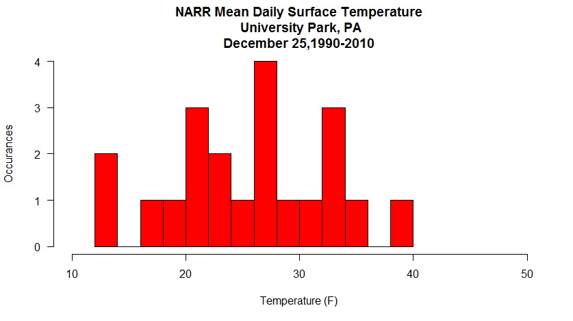
Let's consider the problem that we want to retrieve the Christmas Day mean surface temperatures for University Park, PA for the years 1990 through 2010. How might we do that in an automated manner? Let's look at some code... (Don't forget to set your working directory!)
# if for some reason we need to reinstall the
# package, then do so.

if (!require("ncdf4")) {
  install.packages("ncdf4") }

library(ncdf4)

# specify the file name and location URL
filename<-"air.sfc.1990.nc"
saved_filename<-"air.sfc.1990mean.nc"
url <- "ftp://ftp.cdc.noaa.gov/Datasets/NARR/Dailies/monolevel/"

# get the file... the mode MUST be "wb" (write binary)
download.file(paste0(url,filename), saved_filename, quiet = FALSE, mode="wb")

# open the file
nc <- nc_open(saved_filename)

# print some info to show a good retrieval
print(head(nc$dim$time$vals))

# close the file
nc_close(nc)

# delete the file (this is optional)
file.remove(saved_filename)
Notice in this code we send the filename and its location to a function: download.file(...) which fetches the file and places it in your working directory (as a default). There are numerous parameters that can be set but notice that you can control the saved file name as well as the appearance of the progress bar via the quiet parameter. In fact, we can get quite fancy here if we want. For example, I can create a sub-directory (manually) named "data" within the working directory where I can store the data files that I download (by adding "data/" to the saved file name). I can also check to see if the file I want to download already exists in my directory by using the file.exists(...) function. See the modified code snippet below that only downloads the file if it doesn't exist in the "data/" subdirectory. Note that I have commented out the file.remove(saved_filename) command at the end of the script. In this context (and for the sake of speed) I want to keep the files that I download, but when I run the script for real, I will delete them to save space (it will take much longer to run the script though).
filename<-"air.sfc.1990.nc"
saved_filename<-"data/air.sfc.1990.nc"
url <- "ftp://ftp.cdc.noaa.gov/Datasets/NARR/Dailies/monolevel/"

# get the file... the mode MUST be "wb" (write binary)
if(!file.exists(saved_filename)) {
    download.file(paste0(url,filename), saved_filename, quiet = FALSE, mode="wb")
}
Are you getting a feel for where this is going? If we could create a list of filenames to retrieve then we could loop over those names and retrieve the information we need for each year. This is easy and can be accomplished by these three lines located right after the library call...
dates<-seq(1990,2010,1)
in_file_list<-paste0("air.sfc.",dates,".nc")
out_file_list<-paste0("air.sfc.",dates,"mean.nc")
Run these three lines of code and look at the variables in_file_list and out_file_list in the environment inspector. Easy, right? Now, we need the automation part... do you remember how to do it? We put everything that we want to automate and place it in a function. Then we run the command: mapply(...) with the function name and the variables we want to send the function. Here are the basics...
# ALL THE HEADER STUFF GOES HERE

# get our list of dates (keep the list short for testing)
dates<-seq(1990,1992,1)
in_file_list<-paste0("air.sfc.",dates,".nc")
out_file_list<-paste0("air.sfc.",dates,"mean.nc")
url <- "ftp://ftp.cdc.noaa.gov/Datasets/NARR/Dailies/monolevel/"

# make a placeholder for the specific point data we want
narr.timeseries <- data.frame()

# make the retrieve function
retrieve_data <- function(filename, saved_filename) {
  #
  # PUT ALL THE AUTOMATION STUFF IN HERE
  #
}

# call the automation function with the in and out file lists
mapply (retrieve_data, in_file_list, out_file_list)

# ALL THE PLOT STUFF GOES HERE
All that's left is for you to build the data retrieval code in the automation section and add a plot function after the mapply(...). Can you do it? You've done all the pieces before, and there's a small issue or two to sort out... but give it a try. My version of the Christmas daily mean temperatures histogram is below. If you get stuck, I have put my complete copy of the code in the Quiz Yourself section.
Quiz Yourself...
Were you able to figure everything out? If not, click on the bar below to reveal my complete code. Remember (yes, I forgot) that inside of the automation function all of the variables disappear every time the function restarts. If you want to access a variable after the function finished (called a global variable), you must use the "<<-" assignment operator, not just "<-".
# if for some reason we need to reinstall the
# package, then do so.

if (!require("ncdf4")) {
  install.packages("ncdf4") }

library(ncdf4)

# Set up my date range and file info
dates<-seq(1990,2010,1)
in_file_list<-paste0("air.sfc.",dates,".nc")
out_file_list<-paste0("data/air.sfc.",dates,"mean.nc")
url <- "ftp://ftp.cdc.noaa.gov/Datasets/NARR/Dailies/monolevel/"

# choose a day and location
target_datetime<-"12-25"
location<-c(40.85, -77.85)

# This will be our placeholder for the specific point data we want
narr.timeseries <- data.frame()

# we are going to only compute the cloest_point once,
# so let's delete any old versions.
if (exists("closest_point")) { rm(closest_point) }

retrieve_data <- function(filename, saved_filename) {

# get the file
if(!file.exists(saved_filename)) {
  print(paste0("Retrieving <", filename, "> ... Saving <",saved_filename, ">"))
    download.file(paste0(url,filename), saved_filename, quiet = TRUE, mode="wb")
}

  # open the file
  nc <- nc_open(saved_filename)
  data_dims<-nc$var$air$varsize

  #Get the properly formatted date strings/target time index
  ncdates<-nc$dim$time$vals  #hours since 1800-1-1
  origin<-as.POSIXct('1800-01-01 00:00:00', tz = 'UTC')
  ncdates<-origin + ncdates*(60*60)

  # time_index may change due to leap days so we have to calulate it every time
  time_index<-which(strftime(ncdates,format="%m-%d")==target_datetime)

  # lat and lon index will not change, let's find it only once
  if (!exists("closest_point")) {
    lats<-ncvar_get(nc, varid = 'lat',
                     start = c(1,1),
                     count = c(data_dims[1],data_dims[2]))

    lons<-ncvar_get(nc, varid = 'lon',
                     start = c(1,1),
                     count = c(data_dims[1],data_dims[2]))
    lons<-ifelse(lons>0,lons-360,lons)

    distance<-(lats-location[1])**2+(lons-location[2])**2

  # I want closest_point defined outside of the function (global) so I used <<-
    closest_point<<-which(distance==min(distance), arr.ind = TRUE)
  }

  temp_out<-array(data = NA, dim = c(1,1,1))

  temp_out[,,]<-ncvar_get(nc, varid = 'air',
                            start = c(closest_point[1],closest_point[2],time_index),
                            count = c(1,1,1))
  temp_out[,,]<-(temp_out[,,]-273.15)*9/5+32

  # add the row to the data frame
  row <- data.frame(Year=strftime(ncdates[time_index], format="%Y"), Temperature=temp_out[1,1,1])

  # use the global variable
  narr.timeseries <<- rbind(narr.timeseries,row)

  # close the file
  nc_close(nc)

  # delete the file (optional)
  file.remove(saved_filename)

}

# The main loop
mapply (retrieve_data, in_file_list, out_file_list)

# Write the data out to a file (just so we don't have to calculate it again
write.csv(narr.timeseries, "data/christmas_temps.csv")

# converts $Year from a factor to a number
# need this if you want a line/scatter plot
narr.timeseries$Year<-as.numeric(levels(narr.timeseries$Year))[narr.timeseries$Year]

# I think a histogram makes more sense here than a line/scatter plot
hist(narr.timeseries$Temperature,
     ylab = "Occurances", xlab = "Temperature (F)",
     main = paste0("NARR Mean Daily Surface Temperature\n University Park, PA\n",
            "December 25,", head(narr.timeseries$Year,1),"-",tail(narr.timeseries$Year,1)),
     las=1,
     breaks=10,
     col="red",
     xlim=c(10,50)
)
To GRIB or not to GRIB
Prioritize...
The ability to decode GRIB files crosses perhaps the final boundary of data retrieval methods. However, there are significant technical hurdles that must overcome in order to do so. Therefore, I am labeling this section as an Explore Further (rather than a required reading). If you are interested in retrieving, decoding, and working with data in GRIB format, you should invest some time in figuring out an acceptable workflow. If you are a casual user, however, I suggest experimenting with these data, but don't give yourself a headache.
Explore Further...
As I mentioned in the beginning of this lesson, the "raw"-est form of environmental data you'll run across is likely to be the WMO standard GRIdded Binary (GRIB) data. I say "raw" because GRIB files were not created with the casual end-user in mind. The GRIB format was created for transmitting large volumes of gridded data via computer-to-computer communications. GRIB also serves as an efficient storage and retrieval data format and is specially designed for use in autonomous systems. What this all means for you and me is that we are not meant to be rooting around inside GRIB files (Is it a secret club?... maybe). If you are so inclined, peruse the GRIB User's Guide [22]. However, don't delve too deeply because we are going to get some tools to help us decode the raw files into something more meaningful.
We will explore two possible approaches for reading GRIB files. Both involve installing other tools to decode the files and convert them into something more meaningful.
Method 1: WGRIB/WGRIB2
The first place I started looking was R libraries to handle GRIB files. There are some out there, and you are welcome to play around with them (rNomads even has some built-in GRIB functions). Many of these R libraries, however, are merely wrappers that execute exterior tools (and to make matters worse, I found significant compatibility issues when trying to run pre-built commands). That said, I was able to read and plot GRIB files from the NARR. Let me show you how.
First, we need some data to play with. The GRIB versions of the NARR are hosted by the NCAR/UCAR Research Data Archive [23]. In fact, there are many different types of data housed at this site (feel free to browse). You will need to register but the account is free, so go ahead and do that now. After you are registered, proceed to the NARR page [13] and after reading about the data set, click on the "Data Access" tab and then on the "regrouped 3-hourly files". To start, go to "Faceted Browse", then pick a single date before hitting continue. On the next page, select "Temperature" from the parameter list, and "Ground or water surface" from the level list. Click on the "Update the List" button and then select one of the files below (it doesn't really matter for our example... each file spans 10 days). Download the compressed ".tar" file and extract the contents in your target directory. You should have a directory of filenames that look like "merged_AWIP32.2017030100.RS.sfc". Copy one of those files to your R-script directory (just to make it easy).
Now that we have the data, we need to get the tools that will actually process the GRIB files. We are going to use the Climate Prediction Center's WGRIB and WGRIB2 decoders. Start by going to the WGRIB website [24] and finding the instructions for your operating system. Windows users can get pre-compiled (exe's and dll's); Mac users will need to compile their own. For Windows users (of which I am one), you need to place all of the pre-compiled WGRIB files in a directory (I placed it under "Program Files") and then add that directory to your system path (if you don't know how to do that, just Google it). Now do the same for WGRIB2 by starting at the CPC's WGRIB2 website [25]. You should know that it works when you can type "wgrib" or "wgrib2" in a command window and get a display of the usage instructions (see a picture of mine [26]).
I should point out that there are two different formats for GRIB files. The older one, GRIB1 or just GRIB, and the newer one GRIB2. You must use the proper form of WGRIB/WGRIB2 depending on the file that you want to decode (newer files tend to be GRIB2), but some systems like the NARR still use the older GRIB format (for compatibility, I suspect). Generally, the site you download from will tell you, but you'll know if you are using the wrong command if you get a "not in GRIB format" type of error. If you stumble upon files in a GRIB2 format, it's an easy fix, you just have to replace wgrib with wgrib2 for all of the code below.
Whew! The good news is that we are over the hump in terms of the technical stuff. Now, let's plot the data. Open a new R-script, and enter the following lines of code:
# set the file name
grib.file<-"merged_AWIP32.2017030100.RS.sfc"

# query the GRIB file for the headers
file.info<-shell(paste0("wgrib -s ", grib.file), shell=NULL, flag="", intern = TRUE, wait = TRUE)
These three lines first define a file name and variable name. Then we run the external program wgrib command using R's shell(...) function. Basically, this function is the same as running wgrib -s merged_AWIP32.2017030100.RS.sfc from a command prompt window, except we can capture the result and paste it into the R-object: file.info. Take a look at file.info... it's a listing of the file's record headers. To interpret them, you can read WGRIB's user's guide [27]. The important thing to note is the variable and level information stored in each record. Now we can run the next four commands in our script:
# specify the variable/level I want
var<-"TMP:sfc"

# run wgrib decoding the proper record and write output file
shell(paste0("wgrib -d ", grep(var, file.info), " -text -o wgrib_output.txt ", grib.file), shell=NULL, flag="", intern = TRUE, wait = TRUE)

# read the output file into R
values<-read.csv("wgrib_output.txt")

# delete the output file (we don't need it anymore)
file.remove("wgrib_output.txt")
First, we define the variable string we want (by browsing the file.info table). Note that if we already know what we want, there's no need to even collect file info at all. Next, we run a shell command again telling wgrib that we want to decode "-d" the record number containing the variable string (that's what grep(...) gives us). We want the output to be "-text" and the output to be sent to "wgrib_output.txt". All that's left to do is read in the output file and then delete it (because we don't need it anymore). The variable values is a data frame with a single column of numbers rather than a grid, so now we need to fix that before we plot it.
# Replace the missing value: 999999 with NA
values$X349.277[which(values$X349.277>500)]<-NA

# convert from K to degrees F
values$X349.277<-(values$X349.277-273.15)*9/5+32

# make the single column into a matrix (grid)
grid=matrix(values$X349.277, nrow=349, ncol=277)
So how do we know how many rows and columns the data are? And even more important, what are the latitudes and longitudes of each point? These GRIB data grids don't contain any specific spatial information because it is assumed that you know this already. So how do we figure this out? First, we know from previous explorations that NARR data is generated on a 349x277 grid with a Lambert conformal projection. We know this from the NARR documentation and also from a more thorough investigation of the GRIB header information (try: wgrib -V merged_AWIP32.2017030100.RS.sfc and see what you get.). Furthermore, we previously generated the lat/lon grids from one of the NetCDF files. You can run one of these scripts again to strip out the lat and lon from the NetCDF files, or you can simply create an R-data object that contains those variables. I saved those two lat/lon grids as an R-object that you can just load into your current script. Copy this file: narr_lats_lons.RData [28] into your working directory and add the line: load("narr_lats_lons.RData") to the top of your script. Notice when you source the script, variables lats and lons now appear in the Environment tab.
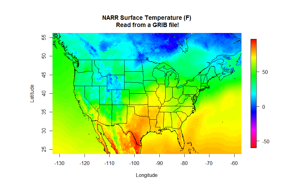
Finally, you can read the latitude and longitude in from another GRIB file. This file contains all of the constant fields of the NARR [29] such as the elevation, soil type and lat/lon of each grid point (you want to grab the file named "rr-fixed.grb". You can read in these fields just as you did the temperature data and then make your plot. Give it a try, you should have all the pieces to produce the plot below. Start with the NetCDF plotting code and swap the GRIB lines. If you need a hint, click below to reveal the code (one for reading the lat/lon values and one for reading and plotting the NARR data).
# THIS SCRIPT READS IN THE FIXED VALUES GRIB
# FILE TO RETRIEVE THE LATITUDE AND LONG GRIDS

# set the file name
grib.file<-"rr-fixed.grb"

# specify the latitude variable
var<-"NLAT:sfc"

# query the GRIB file for the headers
file.info<-shell(paste0("wgrib -s ", grib.file), shell=NULL, flag="", intern = TRUE, wait = TRUE)

# run wgrib decoding the latitudes and write output file
shell(paste0("wgrib -d ", grep(var, file.info), " -text -o wgrib_output.txt ", grib.file), shell=NULL, flag="", intern = TRUE, wait = TRUE)

# read the output file into R
grib_lats<-read.csv("wgrib_output.txt")

# delete the output file (we don't need it any more)
file.remove("wgrib_output.txt")

# specify the longitude variable
var<-"ELON:sfc"

# run wgrib decoding longitude and write output file
shell(paste0("wgrib -d ", grep(var, file.info), " -text -o wgrib_output.txt ", grib.file), shell=NULL, flag="", intern = TRUE, wait = TRUE)

# read the output file into R and delete it
grib_lons<-read.csv("wgrib_output.txt")
file.remove("wgrib_output.txt")

# make the single columns into matrices (grid)
grid_lats=matrix(grib_lats$X349.277, nrow=349, ncol=277)
grid_lons=matrix(grib_lons$X349.277, nrow=349, ncol=277)

# swap the longitudes for the map routine
grid_lons<-grid_lons-360

# remove the objects that we don't need anymore
rm(grib_lats, grib_lons)
# THIS SCRIPT READS NARR DATA FROM A GRIB FILE

# We'll need these libraries for plotting
library(fields)
library(maps)

# Read and process the lat/lon script first
source("read_lat_lon.R")

# set the file name
grib.file<-"merged_AWIP32.2017030100.RS.sfc"

# query the GRIB file for the headers
file.info<-shell(paste0("wgrib -s ", grib.file), shell=NULL, flag="", intern = TRUE, wait = TRUE)

# specify the variable/level I want
var<-"TMP:sfc"

# run wgrib decoding the proper record and write output file
shell(paste0("wgrib -d ", grep(var, file.info), " -text -o wgrib_output.txt ", grib.file), shell=NULL, flag="", intern = TRUE, wait = TRUE)

# read the output file into R
values<-read.csv("wgrib_output.txt")

# delete the output file (we don't need it any more)
file.remove("wgrib_output.txt")

# Replace the missing value: 9.99E+20 with NA
values$X349.277[which(values$X349.277>50000)]<-NA

# convert from K to degrees F
values$X349.277<-(values$X349.277-273.15)*9/5+32

# make the single column into a matrix (grid)
grid=matrix(values$X349.277, nrow=349, ncol=277)

# plot the data
colormap<-rev(rainbow(100))

# Note: Remember, if you get an error that says, "plot too large"
# either expand your plot window, or reduce the "pin" values
par(pin=c(6.25,4))

image.plot(grid_lons, grid_lats, grid, col = colormap,
           xlim=c(-130,-60), ylim=c(25,55),
           xlab = "Longitude", ylab = "Latitude",
           main = "NARR Surface Temperature (F)\n Read from a GRIB file!")

# draw the map
map('state', fill = FALSE, col = "black", add=TRUE)
map('world', fill = FALSE, col = "black", add=TRUE)
Method 2: DEGRIB
We saw in the first method that R has no native functions that can decode GRIB files, and thus we need to interface with some tools to help up do so. We were able to use R to automate the calling of either "wgrib.exe" or "wgrib2.exe" by using the shell command. The output of these GRIB decoders is fed into a file which is then read back into R. The advantage of this method is that many operations can be automated, extracting and analyzing large quantities of data. However, technical considerations may limit the effectiveness of this approach.
A second method is to first decode the GRIB files manually into a format better suited for R. This method also uses a third-party tool but is not called by the R program. Its implementation is far more straightforward (in most cases) but in my opinion less powerful because of the lack of automation available. The utility that we are going to use is called DEGRIB [30] and is available from the Meteorological Development Laboratory of the National Weather Service. It was initially developed for decoding output from the National Forecast Database. However, it is a great tool for decoding both GRIB1 and GRIB2 files. Start with the installation instructions [31]... if you have Windows or Linux, the process is relatively simple (with a Mac, it may be more complex). You eventually want to run the program "tkdegrib.exe".
Once in the program, select the "GIS" tab and then use the top portion of the GUI window [32] to navigate to the proper folder/file. The file details appear in the middle section of where you can choose one of the records to decode. Finally, choose an export method (lower-left... I recommend either .csv or NetCDF) and adjust your precision and units in the lower right and generate your file. You can now load this file into R using the methods that you already know. One advantage of this method is that you also get latitude and longitude columns along with your selected data. Give it a try if you like!
Thoughts on Reanalysis Datasets
Prioritize...
As with all data, care must be taken not to assume too much with regards to what information reanalysis products can provide. In this section, I provide a few reading assignments that revisit the pros and cons of how reanalysis data sets can be useful.
Read...
In this lesson, we have been playing around with reanalysis data sets as a means of learning about NetCDF and GRIB file formats. All along I have cautioned you about not treating reanalysis data as an observational data set -- they are not. Yet, reanalysis data sets can (and do) provide us with remarkably accurate records of the past atmospheric state, in a temporally coherent and spatially gridded format. While I wouldn't use reanalysis output to construct a daily record of temperature for a certain location, I might consider using such data to reconstruct a reasonably accurate climatology, especially when observations are lacking.
The Climate Data Guide from NCAR/UCAR [33] has a wealth of global data sets, including an excellent series of pages on reanalysis data sets. Rather than reinvent their thoughts and findings, I will send you there in the following reading assignment.
Reading Assignment
From the Climate Data Guide from NCAR/UCAR read...
- Atmospheric Reanalysis Overview [34] (including the table of available reanalysis data)
- Expert Guidance Section [35] for the Reanalysis Overview
Lesson 6 Activity
Assignment Objective...
You will use the knowledge and scripts you have gained from this lesson to assess feasibility of using reanalysis climatology in data-sparse regions.
Let's get started.
Setup...
In this lesson, we practiced retrieving data from NetCDF and GRIB files by looking at the North American Regional Reanalysis data set. One might argue the need for such a data set as a historical reference over observation-rich regions. However, over the oceans, NARR data may be the only source of climatological data available. But how accurate are the data? In this assignment, we will examine a host of observations from ocean buoys and then compare those observations with NARR data. Our goal is not necessarily to make fine-scale comparisons, but rather determine on what scales the NARR data are an acceptable proxy for climatologies over the oceans.
Deliverables...
Please use R to answer the questions posed below. In some cases, you will need to paste the output from R, and in other cases, you will need to provide a written analysis along with a graphic or two.
Questions...
- Use the ISD map-generating code located in Lesson 3 to locate a buoy or offshore observing platform off the coast of the United States (in the Atlantic, Pacific, or Gulf of Mexico). Note: The further offshore the better (greater than 100 miles) and choose a station that has been in operation for at least 10 years. Do some research to find out what you can about this observing platform. You might want to visit the National Data Buoy Center [36] to see if you can locate your station and determine what type of instrumentation that it provides. Write up a brief description of what you discover. Is this observing platform a reliable "ground truth" for the comparison that we will be making?
- Retrieve the ISD data from your offshore station for a recently completed year. You're going to want air temperature, sea-surface temperature, wind speed and wind direction. Please retrieve all of the quality flags too, so that you can throw out everything that is flagged as suspicious. Provide 1) a graph of air temperature and sea-surface temperature for the year and 2) a wind rose for the year.
Here's the algorithm I used to retrieve/format the ISD data...
# check to see if rnoaa has been installed # add the library and NOAA key # Get the ISD data # Grab the following columns # Note: your station might not have all of these isd_trimmed <- isd_data[c("date","time", "wind_direction","wind_direction_quality", "wind_speed", "wind_code", "wind_speed_quality", "temperature","temperature_quality", "SA1_temp","SA1_quality")] # Throw out all values where the quality flag is not "1" # You might find that "9" is acceptable for SA1_temp # You can check your data first with: table(isd_trimmed$temperature_quality) # This shows you how many of each temperature quality flags you have isd_trimmed$temperature[isd_trimmed$temperature_quality!=1]<-NA isd_trimmed$SA1_temp[isd_trimmed$SA1_quality!=9]<-NA # Fix the wind values so that calm winds have speed=0 # and direction=NA # Fix the date/time code # Change the coded values to actual values # make a new data frame for the windRose plot (remember it's picky) # Put your plotting code here - Now, retrieve the corresponding NARR data for your chosen year and the lat/lon of your station. You want the highest temporal resolution available (the 3 hourly files). You want the surface temperature, 2-m air temperature and the U- and V-winds at 10m. Models compute the N/S (v-wind) and E/W (u-wind) components of the wind rather than speed and direction. Once you modify and run the two scripts below, generate a temperature plot and windrose similar to the ones above. What do you observe?
Algorithm for the NARR temperature retrievals...
# load ncdf4 if we need to
# include the library

# open the two temperature CDF files

# set the location of our station

# determine the dimensions of the data set?

#Get the properly formatted date strings

# obtain the lat/lon grids

# find the grid index of closest point

# create the temperature arrays... Notice the different dim parameter
temp2m_out = array(data = NA, dim = c(1,1,data_dims[3]))
tempsfc_out = array(data = NA, dim = c(1,1,data_dims[3]))

# load the 2m temperature array and convert it to C

# load the sfc temperature array and convert it to C

# Make a new dataframe to hold the data

# Put any plotting codes here
Algorithm for the NARR Wind retrieval...# load ncdf4 if we need to # include the library # open the two wind CDF files # set the location of our station # determine the dimensions of the data set? #Get the properly formatted date strings # obtain the lat/lon grids # Find the grid index of closest point # Create the wind arrays # load the u-wind array uwind_out[,,] = ncvar_get(nc1, varid = 'uwnd', start = c(closest_point[1],closest_point[2],1), count = c(1,1,data_dims[3])) # get the v-wind array vwind_out[,,] = ncvar_get(nc2, varid = 'vwnd', start = c(closest_point[1],closest_point[2],1), count = c(1,1,data_dims[3])) # Calculate speed and direction from U and V components NARR_windsp<-sqrt(uwind_out[1,1,]^2+vwind_out[1,1,]^2) NARR_winddir<-(270-(atan2(vwind_out[1,1,],uwind_out[1,1,])*(180/pi)))%%360 # Create a new dataframe with the final data NARR_wind_data<-data.frame(ncdates,NARR_winddir,NARR_windsp) colnames(NARR_wind_data)<- c("timecode","wd","ws") # Put the windRose(...) plotting code here - Now, you are going to be asked to argue whether the NARR data over this part of the ocean might be a good proxy for in situ observations (and on what time scales those proxies are suitable). To do this, you are going to need to compare the two sets of of data. You might have noticed that the ISD data are every hour and the NARR data are every 3 hours, and in my case, there are some missing observations in the ISD data. So, if you wanted to do a direct comparison, you will need to use only the dates/times common to both files. Fortunately, R has a function that's called
merge(...)that does exactly this. I have provided a few more lines of code below that will help you merge your data together. Show a scatter plot ofall_data$T2mvsall_data$temperature, orall_data$SSTvsall_data$SA1_temp. What do these graphs tell you about the comparability of the model data versus the observations? Plot the error between observation and model. Is a histogram a good way to do this? How about the error as a function of model temperature (maybe a box plot)?Merge code...> # First let's merge all of the NARR data together > all_data<-merge(NARR_temp_data, NARR_wind_data, by="timecode", all=FALSE) > # Now merge in the ISD data > all_data<-merge(all_data,isd_trimmed, by="timecode", all=FALSE)
- How do we change the time scales of the observations? Again, R comes to the rescue with the
aggregate(...)function. Use the code below as a template to compare the daily means for air temperature and sea-surface temperature. What do you observe? Is one measurement more in agreement than the other? If so, speculate on why that might be.Aggregate code...# sample aggregate function. daily_temp_means<-aggregate(cbind(T2m,temperature)~format(all_data$timecode, "%m-%d"), data=all_data, FUN=mean, na.rm=TRUE) # Note how this function works... # cbind(... lists the columns to compute # ~format(... gets a list of month-date (this is the "aggregate by" variable) # data=... this is the data frame to aggregate # FUN=... the function to apply (you can also try "max" or "min") # na.rm... removes any NA's from the aggregating process
- Modify the aggregate code to create a
daily_windsp_meansdataset. Make a scatter plot comparing model and observed daily mean wind speeds and comment about what you observe. Can you think of a reason for the difference (hint: consider where the model is computing the wind speed versus where it is observed). How might you correct for this difference? - Extra Credit: Note that I didn't have you compute means of wind direction (in the format it is now). Why is that? What errors might arise? How might we obtain accurate means of wind direction. Write a snippet of R code to do this given just wind speed and direction.
The Fine Print...
- Please submit your report in either MSWord or PDF format.
- Saving images: R-Studio makes saving graphs a piece of cake. Notice that at the top of the plot window there is an "Export" pull-down where "Save as Image" is an option. When you choose "Save as image", you are given a dialog box where you can set the type (PNG is best), location, and filename of your image. I would set aside a folder for this assignment where you can save your images and then paste them into your word-processing document.
- Proofreading is a must. It shows professionalism and care for your work. This includes not only basic spelling and grammar, but readability as well. If you struggle with proofreading, have someone give your draft a once-over and provide suggestions.
- Grading: I want to foster an environment where you can focus more on what you are learning than what "grade" you are getting. However, that said, I have to give some sort of grade and feedback for each assignment. Please see my assignment grading rubric in the Orientation section for general guidelines on assignment grades.