Chapter 1 outlined several of the distinguishing properties of geographic data. One is that geographic data are necessarily generalized, and that generalization tends to vary with scale. A second distinguishing property is that the Earth's complex, nearly-spherical shape complicates efforts to specify exact positions on Earth's surface. This chapter explores implications of these properties by illuminating concepts of scale, Earth geometry, coordinate systems, the "horizontal datums" that define the relationship between coordinate systems and the Earth's shape, and the various methods for transforming coordinate data between 3D and 2D grids, and from one datum to another.

Compared to Chapter 1, Chapter 2 may seem long, technical, and abstract, particularly to those for whom these concepts are new. 

Objectives

Students who successfully complete Chapter 2 should be able to:

1. demonstrate your ability to specify geospatial locations using geographic coordinates;
2. convert geographic coordinates between two different formats;
3. explain the concept of a horizontal datum;
4. calculate the change in a coordinate location due to a change from one horizontal datum to another;
5. estimate the magnitude of "datum shift" associated with the adjustment from NAD 27 to NAD 83;
6. recognize the kind of transformation that is appropriate to georegister two or more data sets;
7. describe the characteristics of the UTM coordinate system, including its basis in the Transverse Mercator map projection;
8. plot UTM coordinates on a map;
9. describe the characteristics of the SPC system, including map projection on which it is based;
10. convert geographic coordinates to SPC coordinates;
11. interpret distortion diagrams to identify geometric properties of the sphere that are preserved by a particular projection; and
12. classify projected graticules by projection family.

"Try This!" Activities

Take a minute to complete any of the Try This activities that you encounter throughout the chapter. These are fun, thought-provoking exercises to help you better understand the ideas presented in the chapter.

This textbook is used as a resource in Penn State's Online Geospatial Education online degree and certificate programs. If this topic is interesting to you and you want to learn more about online GIS and GEOINT education at Penn State, check out our Geospatial Education Program Office.

You hear the word "scale" often when you work around people who produce or use geographic information. If you listen closely, you'll notice that the term has several different meanings, depending on the context in which it is used. You'll hear talk about the scales of geographic phenomena and about the scales at which phenomena are represented on maps and aerial imagery. You may even hear the word used as a verb, as in "scaling a map" or "downscaling." The goal of this section is to help you learn to tell these different meanings apart, and to be able to use concepts of scale to help make sense of geographic data.

Specifically, in this part of Chapter 2  you will learn to:

1. calculate map scale using representative fractions;
2. describe the general relationship between map scale, detail, and accuracy.

Often "scale" is used as a synonym for "scope" or "extent." For example, the title of an international research project called The Large Scale Biosphere-Atmosphere Experiment in Amazonia (1999) uses the term "large scale" to describe a comprehensive study of environmental systems operating across a large region. This usage is common not only among environmental scientists and activists, but also among economists, politicians, and the press. Those of us who specialize in geographic information usually use the word "scale" differently, however.

When people who work with maps and aerial images use the word "scale," they usually are talking about the sizes of things that appear on a map or air photo, relative to the actual sizes of those things on the ground.

Map scale is the proportion between a distance on a map and a corresponding distance on the ground:

(D_m / D_g).

By convention, the proportion is expressed as a "representative fraction" in which map distance (D_m) is reduced to 1. The proportion, or ratio, is also typically expressed in the form 1 : D_g rather than 1 / D_g.

The representative fraction 1:100,000, for example, means that a section of road that measures 1 unit in length on a map stands for a section of road on the ground that is 100,000 units long.

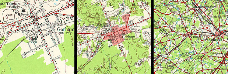
If we were to change the scale of the map such that the length of the section of road on the map was reduced to, say, 0.1 units in length, we would have created a smaller-scale map whose representative fraction is 0.1:100,000, or 1:1,000,000. When we talk about large- and small-scale maps and geographic data, then, we are talking about the relative sizes and levels of detail of the features represented in the data. In general, the larger the map scale, the more detail is shown. This tendency is illustrated below in Figure 2.5.1.

Figure 2.5.1 Geographic data are generalized according to scale. 

Credit: Adapted from Thompson, 1988.

One of the defining characteristics of topographic maps is that scale is consistent across each map and within each map series. This isn't true for aerial imagery, however, except for images that have been orthorectified. As discussed in Chapter 6, large scale maps are typically derived from aerial imagery. One of the challenges associated with using air photos as sources of map data is that the scale of an aerial image varies from place to place as a function of the elevation of the terrain shown in the scene. Assuming that the aircraft carrying the camera maintains a constant flying height (which pilots of such aircraft try very hard to do), the distance between the camera and the ground varies along each flight path. This causes air photo scale to be larger where the terrain is higher and smaller where the terrain is lower. An "orthorectified" image is one in which variations in scale caused by variations in terrain elevation (among other effects) have been removed.

You can calculate the average scale of an unrectified air photo by solving the equation S_p = f / (H-h_avg), where f is the focal length of the camera, H is the flying height of the aircraft above mean sea level, and h_avg is the average elevation of the terrain. You can also calculate air photo scale at a particular point by solving the equation S_p = f / (H-h), where f is the focal length of the camera, H is the flying height of the aircraft above mean sea level, and h is the elevation of the terrain at a given point. 

This textbook is used as a resource in Penn State's Online Geospatial Education online degree and certificate programs. If this topic is interesting to you and you want to learn more about online GIS and GEOINT education at Penn State, check out our Geospatial Education Program Office.

Another way to express map scale is with a graphic (or "bar") scale. Unlike representative fractions, graphic scales remain true when maps are shrunk or magnified.

Figure 2.6.1 Graphic Scales

If they include a scale at all, most maps include a bar scale like the one shown above left (Figure 2.6.1). Some also express map scale as a representative fraction. Either way, the implication is that scale is uniform across the map. In fact, except for maps that show only very small areas, scale varies across every map. As you probably know, this follows from the fact that positions on the nearly-spherical Earth must be transformed to positions on two-dimensional sheets of paper. Systematic transformations of this kind are called map projections. As we will discuss in greater depth later in this chapter, all map projections are accompanied by deformation of features in some or all areas of the map. This deformation causes map scale to vary across the map. Representative fractions may, therefore, specify map scale along a line at which deformation is minimal (nominal scale). Bar scales denote only the nominal or average map scale. Variable scales, like the one illustrated above right, show how scale varies, in this case by latitude, due to deformation caused by map projection.

One of the special characteristics of geographic data is that phenomena shown on maps tend to be represented differently at different scales. Typically, as scale decreases, so too does the number of different features and the detail with which they are represented. Not only printed maps, but also digital geographic data sets that cover extensive areas, tend to be more generalized than datasets that cover limited areas.

Accuracy also tends to vary in proportion with map scale. The United States Geological Survey, for example, guarantees that the mapped positions of 90 percent of well-defined points shown on its topographic map series at scales smaller than 1:20,000 will be within 0.02 inches of their actual positions on the map (see the National Geospatial Program Standards and Specifications). Notice that this "National Map Accuracy Standard" is scale-dependent. The allowable error of well-defined points (such as control points, road intersections, and such) on 1:250,000 scale topographic maps is thus 1 / 250,000 = 0.02 inches / D_g or D_g = 0.02 inches x 250,000 = 5,000 inches or 416.67 feet. Neither small-scale maps nor the digital data derived from them are reliable sources of detailed geographic information.

Figure 2.7.1 Areas (in gray) disqualified as potential sites for a low-level radioactive waste storage facility depicted on a small scale map (original 1:1,500,000) mask small suitable areas large enough to contain the 500-acre facility.

Credit: Chem-Nuclear Systems, Inc., 1994

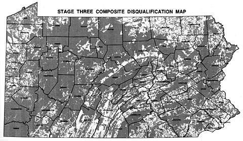
Sometimes the detail lost on small-scale maps causes serious problems. For example, a contractor hired to use GIS to find a suitable site for a low-level radioactive waste storage facility in Pennsylvania presented a series of 1:1,500,000 scale maps at public hearings around the state in the early 1990s. The scale was chosen so that disqualified areas of the entire state could be printed on a single 11 x 17-inch page. A report accompanying the map included the disclaimer that "it is possible that small areas of sufficient size for the LLRW disposal facility site may exist within regions that appear disqualified on the [map]. The detailed information for these small areas is retained within the GIS even though they are not visually illustrated..." (Chem-Nuclear Systems, Inc. 1993, p. 20). Unfortunately for the contractor, alert citizens recognized the shortcomings of the small-scale map, and newspapers published reports accusing the out-of-state company of providing inaccurate documents. Subsequent maps were produced at a scale large enough to discern 500-acre suitable areas.

The term "scale" is sometimes used as a verb. To scale a map is to reproduce it at a different size. For instance, if you photographically reduce a 1:100,000-scale map to 50 percent of its original width and height, the result would be one-quarter the area of the original. Obviously, the map scale of the reduction would be smaller too: 1/2 x 1/100,000 = 1/200,000.

Because of the inaccuracies inherent in all geographic data, particularly in small scale maps, scrupulous geographic information specialists avoid enlarging source maps. To do so is to exaggerate generalizations and errors. The original map used to illustrate areas in Pennsylvania disqualified from consideration for low-level radioactive waste storage shown on an earlier page, for instance, was printed with the statement "Because of map scale and printing considerations, it is not appropriate to enlarge or otherwise enhance the features on this map."

This textbook is used as a resource in Penn State's Online Geospatial Education online degree and certificate programs. If this topic is interesting to you and you want to learn more about online GIS and GEOINT education at Penn State, check out our Geospatial Education Program Office.

The word "scale" can also be used as a synonym for a ruler--a measurement scale. Because data consist of symbols that represent measurements of phenomena, it's important to understand the reference systems used to take the measurements in the first place. In this section, we'll consider a measurement scale known as the geographic coordinate system that is used to specify positions on the Earth's roughly spherical surface. In other sections, we'll encounter two-dimensional (plane) coordinate systems, as well as the measurement scales used to specify attribute data.

In this section of Chapter 2, you will:

1. demonstrate your ability to specify geospatial locations using geographic coordinates;
2. convert geographic coordinates between two different formats.

Figure 2.10.1 A Cartesian coordinate system.

As you probably know, locations on the Earth's surface are measured and represented in terms of coordinates. A coordinate is a set of two or more numbers that specifies the position of a point, line, or other geometric figure in relation to some reference system. The simplest system of this kind is a Cartesian coordinate system (named for the 17th century mathematician and philosopher René Descartes). A Cartesian coordinate system is simply a grid formed by juxtaposing two measurement scales, one horizontal (x) and one vertical (y). The point at which both x and y equal zero is called the origin of the coordinate system. In Figure 2.10.1, above, the origin (0,0) is located at the center of the grid. All other positions are specified relative to the origin. The coordinate of upper right-hand corner of the grid is (6,3). The lower left-hand corner is (-6,-3). If this is not clear, please ask for clarification!

Cartesian and other two-dimensional (plane) coordinate systems are handy due to their simplicity. For obvious reasons, they are not perfectly suited to specifying geospatial positions, however. The geographic coordinate system is designed specifically to define positions on the Earth's roughly-spherical surface. Instead of the two linear measurement scales, x and y, the geographic coordinate systems juxtaposes two curved measurement scales. The east-west scale, called longitude (conventionally designated by the Greek symbol lambda), ranges from +180° to -180°. Because the Earth is round, +180° (or 180° E) and -180° (or 180° W) are the same grid line. That grid line is roughly the International Date Line, which has diversions that pass around some territories and island groups. Opposite the International Date Line is the prime meridian, the line of longitude defined by international treaty as 0°. The north-south scale, called latitude (designated by the Greek symbol phi), ranges from +90° (or 90° N) at the North pole to -90° (or 90° S) at the South pole. We'll take a closer look at the geographic coordinate system next.

Figure 2.10.2 The geographic (or "geodetic") coordinate system.

Figure 2.11.1 The geographic coordinate system.

Credit: David DiBiase

Longitude specifies positions east and west as the angle between the prime meridian and a second meridian that intersects the point of interest. Longitude ranges from +180 (or 180° E) to -180° (or 180° W). 180° East and West longitude together form the International Date Line.

Latitude specifies positions north and south in terms of the angle subtended at the center of the Earth between two imaginary lines, one that intersects the equator and another that intersects the point of interest. Latitude ranges from +90° (or 90° N) at the North pole to -90° (or 90° S) at the South pole. A line of latitude is also known as a parallel.

At higher latitudes, the length of parallels decreases to zero at 90° North and South. Lines of longitude are not parallel but converge toward the poles. Thus, while a degree of longitude at the equator is equal to a distance of about 111 kilometers, that distance decreases to zero at the poles.

This textbook is used as a resource in Penn State's Online Geospatial Education online degree and certificate programs. If this topic is interesting to you and you want to learn more about online GIS and GEOINT education at Penn State, check out our Geospatial Education Program Office.

Geographic coordinates may be expressed in decimal degrees, or in degrees, minutes, and seconds. Sometimes, you need to convert from one form to another. Steve Kiouttis (personal communication, Spring 2002), manager of the Pennsylvania Urban Search and Rescue Program, described one such situation on the course Bulletin Board: "I happened to be in the state Emergency Operations Center in Harrisburg on Wednesday evening when a call came in from the Air Force Rescue Coordination Center in Dover, DE. They had an emergency locator transmitter (ELT) activation and requested the PA Civil Air Patrol to investigate. The coordinates given to the watch officer were 39 52.5 n and -75 15.5 w. This was plotted incorrectly (treated as if the coordinates were in decimal degrees 39.525n and -75.155 w) and the location appeared to be near Vineland, New Jersey. I realized that it should have been interpreted as 39 degrees 52 minutes and 5 seconds n and -75 degrees and 15 minutes and 5 seconds w) and made the conversion (as we were taught in Chapter 2) and came up with a location on the grounds of Philadelphia International Airport, which is where the locator was found, in a parked airliner."

Here's how it works:

To convert -89.40062 from decimal degrees to degrees, minutes, seconds:

1. Subtract the number of whole degrees (89°) from the total (89.40062°). (The minus sign is used in the decimal degree format only to indicate that the value is a west longitude or a south latitude.)
2. Multiply the remainder by 60 minutes (.40062 x 60 = 24.0372).
3. Subtract the number of whole minutes (24') from the product.
4. Multiply the remainder by 60 seconds (.0372 x 60 = 2.232).
5. The result, expressed in the correct number of significant figures, is 89° 24' 2.2" W or S.

To convert 43° 4' 31" from degrees, minutes, seconds to decimal degrees:
DD = Degrees + (Minutes/60) + (Seconds/3600)

1. Divide the number of seconds by 60 (31 ÷ 60 = 0.5166).
2. Add the quotient of step (1) to the whole number of minutes (4 + 0.5166).
3. Divide the result of step (2) by 60 (4.5166 ÷ 60 = 0.0753).
4. Add the quotient of step (3) to the number of whole number degrees (43 + 0.0753).
5. The result, expressed in the correct number of significant figures, is 43.075°

This textbook is used as a resource in Penn State's Online Geospatial Education online degree and certificate programs. If this topic is interesting to you and you want to learn more about online GIS and GEOINT education at Penn State, check out our Geospatial Education Program Office.

Geographic data represent the locations and attributes of things on the Earth's surface. Locations are measured and encoded in terms of geographic coordinates (i.e., latitude and longitude) or plane coordinates (e.g., UTM). To measure and specify coordinates accurately, one first must define the geometry of the surface itself. To see what I mean, imagine a soccer ball. If you or your kids play soccer you can probably conjure up a vision of a round mosaic of 20 hexagonal (six sided) and 12 pentagonal (five sided) panels (soccer balls come in many different designs, but the 32-panel ball is used in most professional matches. Visit Soccer Ball World for more than you ever wanted to know about soccer balls). Now focus on one point at an intersection of three panels. You could use spherical (e.g., geographic) coordinates to specify the position of that point. But if you deflate the ball, the position of the point in space changes, and so must its coordinates. The absolute (though not the relative) position of a point on a surface, then, depends upon the shape of the surface.

Every position is determined in relation to at least one other position. Coordinates, for example, are defined relative to the origin of the coordinate system grid. A land surveyor measures the "corners" of a property boundary relative to a previously-surveyed control point. Surveyors and engineers measure elevations at construction sites and elsewhere. Elevations are expressed in relation to a vertical datum, a reference surface such as mean sea level. As you probably know, there is also such a thing as a horizontal datum, although this is harder to explain and to visualize than the vertical case. Horizontal datums define the geometric relationship between a coordinate system grid and the Earth's surface. Because the Earth's shape is complex, the relationship is too. The goal of this section is to explain the relationship.

Specifically, in this section of Chapter 2 you will learn to:

1. explain the concept of a horizontal datum;
2. calculate the change in a coordinate location due to a change from one horizontal datum to another;
3. estimate the magnitude of "datum shift" associated with the adjustment from NAD 27 to NAD 83.

Figure 2.14.1 The Earth's shape is defined as a surface that closely approximates global mean sea level, but across which gravity is everywhere equal. The caricature of the geoid shown above is not drawn to scale. Irregularities are greatly exaggerated.

Credit: Adapted from Smith, 1988

The accuracy of coordinates that specify geographic locations depends upon how the coordinate system grid is aligned with the Earth's surface. Unfortunately for those who need accurate geographic data, defining the shape of the Earth's surface is a non-trivial problem. So complex is the problem that an entire profession, called geodesy, has arisen to deal with it.

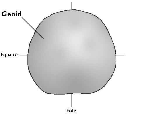
Geodesists define the Earth's surface as a surface that closely approximates global mean sea level, but across which gravity is everywhere equal. They refer to this shape as the geoid. Geoids are lumpy because gravity varies from place to place in response to local differences in terrain and variations in the density of materials in the Earth's interior. Geoids are also a little squat. Sea level gravity at the poles is greater than sea level gravity at the equator, a consequence of Earth's "oblate" shape as well as the centrifugal force associated with its rotation.

Geodesists at the U.S. National Geodetic Survey describe the geoid as an "equipotential surface" because the potential energy associated with the Earth's gravitational pull is equivalent everywhere on the surface. Like fitting a trend line through a cluster of data points, the geoid is a three-dimensional statistical surface that fits as closely as possible gravity measurements taken at millions of locations around the world. As additional and more accurate gravity measurements become available, geodesists revise the geoid periodically. Some geoid models are solved only for limited areas; GEOID03, for instance, is calculated only for the continental U.S.

Recall that horizontal datums define how coordinate system grids align with the Earth's surface. Long before geodesists calculated geoids, surveyors used much simpler surrogates called ellipsoids to model the shape of the Earth.

Figure 2.15.1 Ellipsoids approximate the geoid.

Credit: Adapted from Smith, 1988

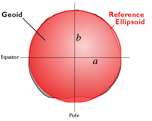
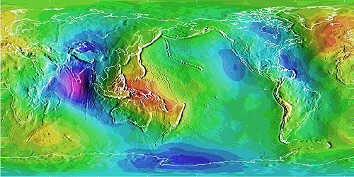
An ellipsoid is a three-dimensional geometric figure that resembles a sphere, but whose equatorial axis (a in Figure 2.15.1, above) is slightly longer than its polar axis (b). The equatorial axis of the World Geodetic System of 1984, for instance, is approximately 22 kilometers longer than the polar axis, a proportion that closely resembles the oblate spheroid that is planet Earth. Ellipsoids are commonly used as surrogates for geoids so as to simplify the mathematics involved in relating a coordinate system grid with a model of the Earth's shape. Ellipsoids are good, but not perfect, approximations of geoids. The map in Figure 2.15.2, below shows differences in elevation between a geoid model called GEOID96 and the WGS84 ellipsoid. The surface of GEOID96 rises up to 75 meters above the WGS84 ellipsoid over New Guinea (where the map is colored red). In the Indian Ocean (where the map is colored purple), the surface of GEOID96 falls about 104 meters below the ellipsoid surface.

Figure 2.15.2 Deviations between an ellipsoid and a geoid.

Credit: National Geodetic Survey, 1997

Many ellipsoids are in use around the world. (Wikipedia presents a list in its entry on Earth Ellipsoids) Local ellipsoids minimize differences between the geoid and the ellipsoid for individual countries or continents. The Clarke 1866 ellipsoid, for example, minimizes deviations in North America. The North American Datum of 1927 (NAD 27) associates the geographic coordinate grid with the Clarke 1866 ellipsoid. NAD 27 involved an adjustment of the latitude and longitude coordinates of some 25,000 geodetic control point locations across the U.S. The nationwide adjustment commenced from an initial control point at Meades Ranch, Kansas, and was meant to reconcile discrepancies among the many local and regional control surveys that preceded it.

The North American Datum of 1983 (NAD 83) involved another nationwide adjustment, necessitated in part by the adoption of a new ellipsoid, called GRS 80. Unlike Clarke 1866, GRS 80 is a global ellipsoid centered upon the Earth's center of mass. GRS 80 is essentially equivalent to WGS 84, the global ellipsoid upon which the Global Positioning System is based. NAD 27 and NAD 83 both align coordinate system grids with ellipsoids. They differ simply in that they refer to different ellipsoids. Because Clarke 1866 and GRS 80 differ slightly in shape as well as in the positions of their center points, the adjustment from NAD 27 to NAD 83 involved a shift in the geographic coordinate grid. Because a variety of datums remain in use, geospatial professionals need to understand this shift, as well as how to transform data between horizontal datums.

The preceding statement remains true despite the fact that NAD 83 will soon be discontinued as part of the National Geodetic Survey's ongoing modernization of the U.S. National Spatial Reference System. The switch from a "passive" ellipsoid-based reference system to a GPS-based dynamic system was planned for 2022, but it has since been delayed until 2024 or -25. Visit the National Geodetic Survey for the latest information. 

Figure 2.16.1 In the U.S., high-order horizontal control point locations are marked with permanent metal "monuments" like the one shown above. The physical manifestation of datum is a network of control point measurements.

Credit: National Geodetic Survey, 2004

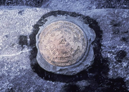
Geoids, ellipsoids, and even coordinate systems are all abstractions. The fact that "horizontal datum" refers to a relationship between an ellipsoid and a coordinate system, two abstractions, may explain why the concept is so frequently misunderstood. Datums do have physical manifestations, however.

Shown above (Figure 2.16.1) is one of the approximately two million horizontal and vertical control points that have been established in the U.S. Although control point markers are fixed, the coordinates that specify their locations are liable to change. The U.S. National Geodetic Survey maintains a database of the coordinate specifications of these control points, including historical locations as well as more recent adjustments. One occasion for adjusting control point coordinates is when new horizontal datums are adopted. Since every coordinate system grid is aligned with an ellipsoid that approximates the Earth's shape, coordinate grids necessarily shift when one ellipsoid is replaced by another. When coordinate system grids shift, the coordinates associated with fixed control points need to be adjusted. How we account for the Earth's shape makes a difference in how we specify locations.

This textbook is used as a resource in Penn State's Online Geospatial Education online degree and certificate programs. If this topic is interesting to you and you want to learn more about online GIS and GEOINT education at Penn State, check out our Geospatial Education Program Office.

GIS specialists often need to transform data from one coordinate system and/or datum to another. For example, digital data produced by tracing paper maps over a digitizing tablet need to be transformed from the tablet's non-georeferenced plane coordinate system into a georeferenced plane or spherical coordinate system that can be georegistered with other digital data "layers." Raw image data produced by scanning the Earth's surface from space tend to be skewed geometrically as a result of satellite orbits and other factors; to be useful these too need to be transformed into georeferenced coordinate systems. Even the point data produced by GPS receivers, which are measured as latitude and longitude coordinates based upon the WGS84 datum, often need to be transformed to other coordinate systems or datums to match project specifications. This section describes three categories of coordinate transformations: (1) plane coordinate transformations; (2) datum transformations; and (3) map projections.

Students who successfully complete this section of Chapter 2 should be able to:
recognize the kind of transformation that is appropriate to georegister two or more data sets.

Some coordinate transformations are simple. For example, the transformation from non-georeferenced plane coordinates to non-georeferenced polar coordinates shown in Figure 2.18.1, below, involves nothing more than the replacement of one kind of coordinates with another.

Figure 2.18.1 The same position specified within two non-georeferenced plane coordinate systems: Cartesian (left) and polar (right).

Credit: Adapted from Iliffe, 2000

Unfortunately, most plane coordinate transformation problems are not so simple. The geometries of non-georeferenced plane coordinate systems and georeferenced plane coordinate systems tend to be quite different, mainly because georeferenced plane coordinate systems are often projected. As you know, the act of projecting a nearly-spherical surface onto a two-dimensional plane necessarily distorts the geometry of the original spherical surface. Specifically, the scale of a projected map (or an unrectified aerial photograph, for that matter) varies from place to place. So long as the geographic area of interest is not too large, however, formulae like the ones described here can be effective in transforming a non-georeferenced plane coordinate system grid to match a georeferenced plane coordinate system grid with reasonable, and measurable, accuracy. We won't go into the math of the transformations here, since the formulae are implemented within GIS software. Instead, this section aims to familiarize you with how some common transformations work and how they may be used.

Similarity Transformation

In the hypothetical illustration below (Figure 2.18.2), the spatial arrangement of six control points digitized from a paper map ("before") are shown to differ from the spatial arrangement of the same points that appear in a georeferenced aerial photograph that is referenced to a different plane coordinate system grid ("after"). If, as shown, the arrangement of the two sets of points differs only in scale, rotation, and offset, a relatively simple four-parameter similarity transformation may do the trick. Your GIS software should derive the parameters for you by comparing the relative positions of the common points. Note that while only six control points are illustrated, ten to twenty control points are recommended (Chrisman 2002).

Figure 2.18.2 Six control point locations before and after a similarity transformation used to correct systematic differences in scale, rotation, and offset between two plane coordinate systems.

Affine Transformation

Sometimes a similarity transformation doesn't do the trick. For example, because paper maps expand and contract more along the paper grain than across the grain in response to changes in humidity, the scale of a paper map is likely to be slightly greater along one axis than the other. In such cases, a six-parameter affine transformation may be used to accommodate differences in scale, rotation, and offset along each of the two dimensions of the source and target coordinate systems. This characteristic is particularly useful for transforming image data scanned from polar-orbiting satellites whose orbits trace S-shaped paths over the rotating Earth.

Figure 2.18.3 Six control point locations before and after an affine transformation used to correct systematic differences in scale, rotation, and offset between two plane coordinate systems. Notice that the arrangement of points before the transformation is skewed as well as offset and rotated.

Second-Order Polynomial Transformation

When neither similarity nor affine transformations yield acceptable results, you may have to resort to a twelve-parameter Second-order polynomial transformation. Their advantage is the potential to correct data sets that are distorted in several ways at once. A disadvantage is that the stability of the results depend very much upon the quantity and arrangement of control points and the degree of dissimilarity of the source and target geometries (Iliffe 2000).

Figure 2.18.4 Six control point locations before and after a second-order polynomial transformation. Notice that the arrangement of points before the transformation is distorted in multiple ways in comparison with the corrected arrangement.

Even more elaborate plane transformation methods, known collectively as rubber sheeting, optimize the fit of a source data set to the geometry of a target data set as if the source data were mapped onto a stretchable sheet.

Root Mean Square Error

GIS software provides a statistical measure of how well a set of transformed control points match the positions of the same points in a target data set. Put simply, Root Mean Square (RMS) Error is the average of the distances (also known as residuals) between each pair of control points. What constitutes an acceptably low RMS Error depends on the nature of the project and the scale of analysis.

This textbook is used as a resource in Penn State's Online Geospatial Education online degree and certificate programs. If this topic is interesting to you and you want to learn more about online GIS and GEOINT education at Penn State, check out our Geospatial Education Program Office.

Point locations are specified in terms of (a) their positions relative to some coordinate system grid and (b) their heights above or below some reference surface. Obviously, the elevation of a stationary point depends upon the size and shape of the reference surface (e.g., mean sea level) upon which the elevation measurement is based. In the same way, a point's position in a coordinate system grid depends on the size and shape of the surface upon which the grid is draped. The relationship between a grid and a model of the Earth's surface is called a horizontal datum. GIS specialists who are called upon to merge data sets produced at different times and in different parts of the world need to be knowledgeable about datum transformations.

NAD 27 to NAD 83

In the U.S., the two most frequently encountered horizontal datums are the North American Datum of 1927 (NAD 27) and the North American Datum of 1983 (NAD 83). The advent of the Global Positioning System necessitated an update of NAD 27 that included (a) adoption of a geocentric ellipsoid, GRS 80, in place of the Clarke 1866 ellipsoid; and (b) correction of many distortions that had accrued in the older datum. Bearing in mind that the realization of a datum is a network of fixed control point locations that have been specified in relation to the same reference surface, the 1983 adjustment of the North American Datum caused the coordinate values of every control point managed by the National Geodetic Survey (NGS) to change. Obviously, the points themselves did not shift on account of the datum transformation (although they did move a centimeter or more a year due to plate tectonics). Rather, the coordinate system grids based upon the datum shifted in relation to the new ellipsoid. And because local distortions were adjusted at the same time, the magnitude of grid shift varies from place to place. The illustrations below compare the magnitude of the grid shifts associated with the NAD 83 adjustment at one location and nationwide.

Figure 2.19.1 A corner of the 1:24,000 scale topographic quadrangle map for State College PA showing the magnitude of grid shift associated with the NAD 83 adjustment. The map is based on NAD 27, but was reprinted with revisions in 1987, including the statement that coordinate system grid lines shift 24 meters west and 5 meters south if NAD 83 coordinates are used instead of NAD 27.

Figure 2.19.2 Magnitude of grid shift associated with the NAD 83 adjustment for the continental 48 U.S. states. Shifts range from 10 to 100 meters in the lower 48 (least in upper Midwest states) to over 200 meters in Alaska, and over 400 meters in Hawaii.

Credit: Dewhurst 1990

Given the irregularity of the shift, NGS could not suggest a simple transformation algorithm that surveyors and mappers could use to adjust local data based upon the older datum. Instead, NGS created a software program called NADCON (Dewhurst 1990, Mulcare 2004) that calculates adjusted coordinates from user-specified input coordinates by interpolation from a pair of 15° correction grids generated by NGS from hundreds of thousands of previously-adjusted control points.

GPS Data and WGS 84

The U.S. Department of Defense created the Global Positioning System (GPS) over a period of 16 years at a startup cost of about $10 billion. GPS receivers calculate their positions in terms of latitude, longitude, and height above or below the World Geodetic System of 1984 ellipsoid (WGS 84). Developed specifically for the Global Position System, WGS 84 is an Earth-centered ellipsoid which, unlike the many regional, national, and local ellipsoids still in use, minimizes deviations from the geoid worldwide. Depending on where a GIS specialist may be working, or what data he or she may need to work with, the need to transform GPS data from WGS 84 to some other datum is likely to arise. Datum transformation algorithms are implemented within GIS software as well as in the post-processing software provided by GPS vendors for use with their receivers. Some transformation algorithms yield more accurate results than others. The method you choose will depend on what choices are available to you and how much accuracy your application requires.

Unlike the plane transformations described earlier, datum transformations involve ellipsoids and are therefore three-dimensional. The simplest is the three-parameter Molodenski transformation. In addition to knowledge of the size and shape of the source and target ellipsoids (specified in terms of semimajor axis, the distance from the ellipsoid's equator to its center, and flattening ratio, the degree to which the ellipsoid is flattened to approximate the Earth's oblate shape), the offset between the two ellipsoids needs to be specified along X, Y, and Z axes. The window shown below (Figure 2.19.3) illustrates ellipsoidal and offset parameters for several horizontal datums, all expressed in relation to WGS 84.

Figure 2.19.3 Datum list window in the Waypoint+ software utility (Hildebrand 1997). NAD 27, NAD 83, and WGS 84 are highlighted. The ellipsoid associated with each datum is named, and its size and shape specified (Delta A and Delta (1/f)x10e4), along with three offset parameters, in meters, relative to WGS 84 (Delta x, Delta y, Delta z).

Credit: Waypoint+ software utility

For larger study areas, more accurate results may be obtained using a seven-parameter transformation that accounts for rotation as well as scaling and offset.

Finally, surface-fitting transformations like the NADCON grid interpolation described above yield the best results over the largest areas.

For routine mapping applications covering relatively small geographic areas (i.e., larger than 1:25,000), the plane transformations described earlier may yield adequate results when datum specifications are unknown and when a sufficient number of appropriately distributed control points can be identified.

This textbook is used as a resource in Penn State's Online Geospatial Education online degree and certificate programs. If this topic is interesting to you and you want to learn more about online GIS and GEOINT education at Penn State, check out our Geospatial Education Program Office.

Latitude and longitude coordinates specify positions in a more-or-less spherical grid called the graticule. Plane coordinates like the eastings and northings in the Universal Transverse Mercator (UTM) and State Plane Coordinates (SPC) systems denote positions in flattened grids. This is why georeferenced plane coordinates are referred to as projected, and geographic coordinates are called unprojected. The mathematical equations used to transform latitude and longitude coordinates to plane coordinates are called map projections. Inverse projection formulae transform plane coordinates to geographic. The simplest kind of projection, illustrated in Figure 2.20.1, below, transforms the graticule into a rectangular grid in which all grid lines are straight, intersect at right angles, and are equally spaced. More complex projections yield grids in which the lengths, shapes, and spacing of the grid lines vary.

Figure 2.20.1 Map projections are mathematical transformations between geographic coordinates and plane coordinates.

If you are a GIS practitioner, you have probably faced the need to superimpose unprojected latitude and longitude data onto projected data, and vice versa. For instance, you might have needed to merge geographic coordinates measured with a GPS receiver with digital data published by the USGS that are encoded as UTM coordinates. Modern GIS software provides sophisticated tools for projecting and unprojecting data. To use such tools most effectively, you need to understand the projection characteristics of the data sets you intend to merge. We'll examine map projections in some detail elsewhere in this chapter. Here, let's simply review the characteristics that are included in the "Spatial Reference Information" section of the metadata documents that (ideally!) accompany the data sets you might wish to incorporate in your GIS. These include:

• Projection Name Most common in the GIS realm is the Transverse Mercator, which serves as the basis of the global UTM plane coordinate system, the U.K. and proposed U.S. National Grids, and many zones in the U.S. State Plane Coordinate system (SPC). Other SPC zones are based upon the Lambert Conic Conformal projection, which like many projections is named for its inventor as well as its projection category (conic) and the geometric properties it preserves (conformal). Much map data, particularly in the form of printed paper maps, are based upon "legacy" projections (like the Polyconic in the U.S.) that are no longer widely used. A much greater variety of projection types tend to be used in small scale thematic mapping than in large scale reference mapping.
• Central Meridian Although no land masses are shown, let's assume that the graticule and projected grid shown above are centered on the intersection of the equator (0 latitude) and prime meridian (0° longitude). Most map projection formulae include a parameter that allows you to center the projected map upon any longitude.
• Latitude of Projection Origin Under certain conditions, most map projection formulae allows you to specify different aspects of the grid. Instead of the equatorial aspect illustrated above, you might specify a polar aspect or oblique aspect by varying the latitude of projection origin such that one of the poles, or any latitude between the pole and the equator, is centered in the projected map. As you might imagine, the appearance of the grid changes a lot when viewed at different aspects.
• Scale Factor at Central Meridian This is the ratio of map scale along the central meridian and the scale at a standard meridian, where scale distortion is zero. The scale factor at the central meridian is .9996 in each of the 60 UTM coordinate system zones since each contains two standard lines 180 kilometers west and east of the central meridian. Scale distortion increases with distance from standard lines in all projected coordinate systems.
• Standard Lines Some projections, including the Lambert Conic Conformal, include parameters by which you can specify one or two standard lines along which there is no scale distortion caused by the act of transforming the spherical grid into a flat grid. By the same reasoning that two standard lines are placed in each UTM zone to minimize distortion throughout the zone to a maximum of one part in 1000, two standard parallels are placed in each SPC zone that is based on a Lambert projection such that scale distortion is no worse than one part in 10,000 anywhere in the zone.

This textbook is used as a resource in Penn State's Online Geospatial Education online degree and certificate programs. If this topic is interesting to you and you want to learn more about online GIS and GEOINT education at Penn State, check out our Geospatial Education Program Office.

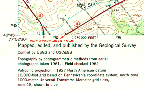
Shown below in Figure 2.21.1 is the southwest corner of a 1:24,000-scale topographic map published by the United States Geological Survey (USGS). Note that the geographic coordinates (40 45' N latitude, 77° 52' 30" W longitude) of the corner are specified. Also shown, however, are ticks and labels representing two plane coordinate systems, the Universal Transverse Mercator (UTM) system and the State Plane Coordinates (SPC) system. The tick labeled "4515" represents a UTM grid line (called a "northing") that runs parallel to and 4,515,000 meters north of, the equator. Ticks labeled "258" and "259" represent grid lines that run perpendicular to the equator and 258,000 meters and 259,000 meters east, respectively, of the origin of the UTM Zone 18 North grid. Unlike longitude lines, UTM "eastings" are straight and do not converge upon the Earth's poles. All of this begs the question, Why are multiple coordinate system grids shown on the map? Why aren't geographic coordinates sufficient?

Figure 2.21.1 Southwest corner of a USGS topographic map showing grid ticks and labels for three different coordinate systems, including the UTM coordinate system.

Credit: USGS. "State College quadrangle, Pennsylvania"

You can think of a plane coordinate system as the juxtaposition of two measurement scales. In other words, if you were to place two rulers at right angles, such that the "0" marks of the rulers aligned, you'd define a plane coordinate system. The rulers are called "axes." The absolute location of any point in the space in the plane coordinate system is defined in terms of distance measurements along the x (east-west) and y (north-south) axes. A position defined by the coordinates (1,1) is located one unit to the right, and one unit up from the origin (0,0). The UTM grid is a widely-used type of geospatial plane coordinate system in which positions are specified as eastings (distances, in meters, east of an origin) and northings (distances north of the origin).

By contrast, the geographic coordinate system grid of latitudes and longitudes consists of two curved measurement scales to fit the nearly-spherical shape of the Earth. As you know, geographic coordinates are specified in degrees, minutes, and seconds of arc. Curved grids are inconvenient to use for plotting positions on flat maps. Furthermore, calculating distances, directions and areas with spherical coordinates are cumbersome in comparison with plane coordinates. For these reasons, cartographers and military officials in Europe and the U.S. developed the UTM coordinate system. UTM grids are now standard not only on printed topographic maps but also for the geospatial referencing of the digital data that comprise the emerging U.S. "National Map."

In this section of Chapter 2, you will learn to:

1. describe the characteristics of the UTM coordinate system, including its basis in the Transverse Mercator map projection; and
2. plot UTM coordinates on a map.

Figure 2.22.1 A Mercator projection of the world, showing the 60 UTM coordinate system zones, each divided into north and south halves at the equator. Also shown are two polar coordinate systems used to specify positions beyond the northern and southern limits of the UTM system.

The Universal Transverse Mercator system is not really universal, but it does cover nearly the entire Earth surface. Only polar areas--latitudes higher than 84° North and 80° South--are excluded. (Polar coordinate systems are used to specify positions beyond these latitudes.) The UTM system divides the remainder of the Earth's surface into 60 zones, each spanning 6° of longitude. These are numbered west to east from 1 to 60, starting at 180° West longitude (roughly coincident with the International Date Line).

The illustration above (Figure 2.22.1) depicts UTM zones as if they were uniformly "wide" from the Equator to their northern and southern limits. In fact, since meridians converge toward the poles on the globe, every UTM zone tapers from 666,000 meters in "width" at the Equator (where 1° of longitude is about 111 kilometers in length) to only about 70,000 meters at 84° North and about 116,000 meters at 80° South.

"Transverse Mercator" refers to the manner in which geographic coordinates are transformed into plane coordinates. Such transformations are called map projections. The illustration below (Figure 2.22.2) shows the 60 UTM zones as they appear when projected using a Transverse Mercator map projection formula that is optimized for the UTM zone highlighted in yellow, Zone 30, which spans 6° West to 0° East longitude (the prime meridian).

As you can imagine, you can't flatten a globe without breaking or tearing it somehow. Similarly, the act of mathematically transforming geographic coordinates to plane coordinates necessarily displaces most (but not all) of the transformed coordinates to some extent. Because of this, map scale varies within projected (plane) UTM coordinate system grids.

The distortion ellipses plotted in red help us visualize the pattern of scale distortion associated with a particular projection. Had no distortion occurred in the process of projecting the map shown in Figure 2.22.2, below, all of the ellipses would be the same size, and circular in shape. As you can see, the ellipses centered within the highlighted UTM zone are all the same size and shape. Away from the highlighted zone, the ellipses steadily increase in size, although their shapes remain uniformly circular. This pattern indicates that scale distortion is minimal within Zone 30, and that map scale increases away from that zone. Furthermore, the ellipses reveal that the character of distortion associated with this projection is that shapes of features as they appear on a globe are preserved while their relative sizes are distorted. Map projections that preserve shape by sacrificing the fidelity of sizes are called conformal projections. The plane coordinate systems used most widely in the U.S., UTM and SPC (the State Plane Coordinates system) are both based upon conformal projections.

Figure 2.22.2 The result of a Transverse Mercator projection of the world centered on UTM Zone 30. Red circles reveal the scale distortion introduced during the transformation from geographic to projected plane coordinates. On the globe, all the circles would be the same size.

The Transverse Mercator projection illustrated above (Figure 2.22.2) minimizes distortion within UTM zone 30. Fifty-nine variations on this projection are used to minimize distortion in the other 59 UTM zones. In every case, distortion is no greater than 1 part in 1,000. This means that a 1,000 meter distance measured anywhere within a UTM zone will be no worse than + or - 1 meter off.

The animation linked to the illustration in Figure 2.22.3, below, shows a series of 60 Transverse Mercator projections that form the 60 zones of the UTM system. Each zone is based upon a unique Transverse Mercator map projection that minimizes distortion within that zone. Zones are numbered 1 to 60 eastward from the international date line. The animation begins with Zone 1.

Figure 2.22.3 One frame of an animation showing a sequence of the 60 Transverse Mercator projections used as the basis of the UTM coordinate system. Highlighted in red is UTM Zone 01, which spans 180° W to 174° W. A unique projection is used for every UTM zone, so that deformation within each zone is minimized.

Map projections are mathematical formulae used to transform geographic coordinates into plane coordinates. (Inverse projection formulae transform plane coordinates back into latitudes and longitudes.) "Transverse Mercator" is one of a hypothetically infinite number of such projection formulae. A visual analog to the Transverse Mercator projection appears below in Figure 2.22.4. Conceptually, the Transverse Mercator projection transfers positions on the globe to corresponding positions on a cylindrical surface, which is subsequently cut from end to end and flattened. In the illustration, the cylinder is tangent to the globe along one line, called the standard line. As shown in the little world map beside the globe and cylinder, scale distortion is minimal along the standard line and increases with distance from it. The animation linked above (Figure 2.22.3) was produced by rotating the cylinder 59 times at an increment of 6°.

Figure 2.22.4 The map above represents a Transverse Mercator projection of the world with a standard meridian at 0° longitude. (Note that because of the very small size of the map, the graticule is shown at 30° resolution.) The globe wrapped in a cylinder is a conceptual model of how the Transverse Mercator projection formula transfers positions on the globe to positions on a plane (The cylinder can be flattened to a plane surface after it is unwrapped from the globe.) The thicker red line on the cylinder and the map is the standard line along which scale distortion is zero. As the distortion ellipses on the map indicate, distortion increases with distance from the standard line.

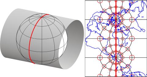
In the illustration above in Figure 2.22.4, there is one standard meridian. Some projection formulae, including the Transverse Mercator projection, allow two standard lines. Each of the 60 variations on the Transverse Mercator projection used as the foundations of the 60 UTM zones employ not one, but two, standard lines. These two standard lines are parallel to, and 180,000 meters east and west of, each central meridian. This scheme ensures that the maximum error associated with the projection due to scale distortion will be 1 part in 1,000 (at the outer edge of the zone at the equator). The error due to scale distortion at the central meridian is 1 part in 2,500. Distortion is zero, of course, along the standard lines.

So, what does the term "transverse" mean? This simply refers to the fact that the cylinder shown above in Figure 2.22.4 has been rotated 90° from the equatorial aspect of the standard Mercator projection, in which a single standard line coincides with 0° latitude.

Figure 2.22.5 The ten UTM zones that span the conterminous U.S.

Credit: U.S. Geological Survey, 2004

One disadvantage of the UTM system is that multiple coordinate systems must be used to account for large entities. The lower 48 United States, for instance, spread across ten UTM zones. The fact that there are many narrow UTM zones can lead to confusion. For example, the city of Philadelphia, Pennsylvania is east of the city of Pittsburgh. If you compare the Eastings of centroids representing the two cities, however, Philadelphia's Easting (about 486,000 meters) is less than Pittsburgh's (about 586,000 meters). Why? Because although the cities are both located in the U.S. state of Pennsylvania, they are situated in two different UTM zones. As it happens, Philadelphia is closer to the origin of its Zone 18 than Pittsburgh is to the origin of its Zone 17. If you were to plot the points representing the two cities on a map, ignoring the fact that the two zones are two distinct coordinate systems, Philadelphia would appear to the west of Pittsburgh. Inexperienced GIS users make this mistake all the time. Fortunately, GIS software is getting sophisticated enough to recognize and merge different coordinate systems automatically.

This textbook is used as a resource in Penn State's Online Geospatial Education online degree and certificate programs. If this topic is interesting to you and you want to learn more about online GIS and GEOINT education at Penn State, check out our Geospatial Education Program Office.

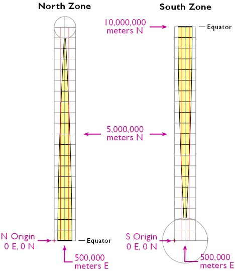
The illustration in Figure 2.23.1, below, depicts the area covered by a single UTM coordinate system grid zone. Each UTM zone spans 6° of longitude, from 84° North and 80° South. Zones taper from 666,000 meters in "width" at the Equator (where 1° of longitude is about 111 kilometers in length) to only about 70,000 meters at 84° North and about 116,000 meters at 80° South. Polar areas are covered by polar coordinate systems. Each UTM zone is subdivided along the equator into two halves, north and south.

Figure 2.23.1 Extent of one UTM coordinate system grid zone. Note that although latitudes are used to specify the extent precisely in relation to the globe, they are geographic, not UTM, coordinates.

The illustration below in Figure 2.23.2 shows how UTM coordinate grids relate to the area of coverage illustrated above in Figure 2.23.1. The north and south halves are shown side by side for comparison. Each half is assigned its own origin. The north south zone origins are positioned to south and west of the zone. North zone origins are positioned on the Equator, 500,000 meters west of the central meridian. Origins are positioned so that every coordinate value within every zone is a positive number. This minimizes the chance of errors in distance and area calculations. By definition, both origins are located 500,000 meters west of the central meridian of the zone (in other words, the easting of the central meridian is always 500,000 meters E). These are considered "false" origins since they are located outside the zones to which they refer. UTM eastings range from 167,000 meters to 833,000 meters at the equator. These ranges narrow toward the poles. Northings range from 0 meters to nearly 9,400,000 in North zones and from just over 1,000,000 meters to 10,000,000 meters in South zones. Note that positions at latitudes higher than 84° North and 80° South are defined in Polar Stereographic coordinate systems that supplement the UTM system.

Figure 2.23.2 UTM coordinate system zone characteristics. Yellow represents areas in which UTM coordinates are valid for a given zone. Red lines parallel to the central meridian represent the two standard lines employed in each Transverse Mercator projection. Each square grid cell in the illustration spans 500,000 meters on each side.

See the Bibliography (last page of the chapter) for further readings about the UTM grid system.

This textbook is used as a resource in Penn State's Online Geospatial Education online degree and certificate programs. If this topic is interesting to you and you want to learn more about online GIS and GEOINT education at Penn State, check out our Geospatial Education Program Office.

The Transverse Mercator projection provides a basis for existing and proposed national grid systems in the United Kingdom and the United States.

In the U.K., topographic maps published by the Ordnance Survey refer to a national grid of 100 km squares, each of which is identified by a two-letter code. Positions within each grid square are specified in terms of eastings and northings between 0 and 100,000 meters. The U.K. national grid is a plane coordinate system that is based upon a Transverse Mercator projection whose central meridian is 2 West longitude, with standard meridians 180 km west and east of the central meridian. The grid is typically related to the Airy 1830 ellipsoid, a relationship known as the National Grid (OSGB36®) datum. The corresponding UTM zones are 29 (central meridian 9° West) and 30 (central meridian 3° West). One of the advantages of the U.K. national grid over the global UTM coordinate system is that it eliminates the boundary between the two UTM zones.

A similar system has been proposed for the U.S. by the Federal Geographic Data Committee. The proposed "U.S. National Grid" is the same as the Military Grid Reference System (MGRS), a worldwide grid that is very similar to the UTM system. As Phil and Julianna Muehrcke (1998, p.p. 229-230) write in the 4th edition of Map Use, "the military [specifically, the U.S. Department of Defense] aimed to minimize confusion when using long numerical [UTM] coordinates" by specifying UTM zones and sub-zones with letters instead of numbers. Like the UTM system, the MGRS consists of 60 zones, each spanning 6° longitude. Each UTM zone is subdivided into 19 MGRS quadrangles of 8° latitude and one (quadrangle from 72° to 84° North) of 12° latitude. The letters C through X are used to designate the grid cell rows from south to north. I and O are omitted to avoid confusion with numbers. Wikipedia offers a good entry on the MGRS here.

This textbook is used as a resource in Penn State's Online Geospatial Education online degree and certificate programs. If this topic is interesting to you and you want to learn more about online GIS and GEOINT education at Penn State, check out ourGeospatial Education Program Office.

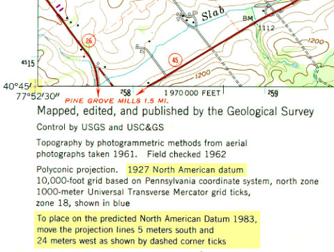
Shown below in Figure 2.25.1 is the southwest corner of a 1:24,000-scale topographic map published by the United States Geological Survey (USGS). Note that the geographic coordinates (40 45' N latitude, 77° 52' 30" W longitude) of the corner are specified. Also shown, however, are ticks and labels representing two plane coordinate systems, the Universal Transverse Mercator (UTM) system and the State Plane Coordinate (SPC) system. The tick labeled "1 970 000 FEET" represents a SPC grid line that runs perpendicular to the equator and 1,970,000 feet east of the origin of the Pennsylvania North zone. The origin lies far to the west of this map sheet. Other SPC grid lines, called "northings" (not shown in the illustration), run parallel to the equator and perpendicular to SPC eastings at increments of 10,000 feet. Unlike longitude lines, SPC eastings and northings are straight and do not converge upon the Earth's poles.

Figure 2.25.1 Southwest corner of a USGS topographic map showing grid ticks and labels for three different coordinate systems, including the SPC coordinate system.

Credit: USGS. "State College Quadrangle, Pennsylvania"

The SPC grid is a widely-used type of geospatial plane coordinate system in which positions are specified as eastings (distances east of an origin) and northings (distances north of an origin). You can tell that the SPC grid referred to in the map illustrated above is the older 1927 version of the SPC grid system because (a) eastings and northings are specified in feet and (b) grids are based upon the North American Datum of 1927 (NAD27). The 124 zones that make up the State Plane Coordinates system of 1983 are based upon NAD 83, and generally use the metric system to specify eastings and northings.

State Plane Coordinates are frequently used to georeference large scale (small area) surveying and mapping projects because plane coordinates are easier to use than latitudes and longitudes for calculating distances and areas. And because SPC zones extend over relatively smaller areas, less error accrues to positions, distances, and areas calculated with State Plane Coordinates than with UTM coordinates.

In this section you will learn to:

1. describe the characteristics of the SPC system, including map projection on which it is based; and
2. convert geographic coordinates to SPC coordinates.

Plane coordinate systems pretend the world is flat. Obviously, if you flatten the entire globe to a plane surface, the sizes and shapes of the land masses will be distorted, as will distances and directions between most points. If your area of interest is small enough, however, and if you flatten it cleverly, you can get away with a minimum of distortion. The basic design problem that confronted the geodesists who designed the State Plane Coordinate System, then, was to establish coordinate system zones that were small enough to minimize distortion to an acceptable level, but large enough to be useful.

The State Plane Coordinate System of 1983 (SPC) is made up of 124 zones that cover the 50 U.S. states. As shown below in Figure 2.26.1, some states are covered with a single zone while others are divided into multiple zones. Each zone is based upon a unique map projection that minimizes distortion in that zone to 1 part in 10,000 or better. In other words, a distance measurement of 10,000 meters will be at worst one meter off (not including instrument error, human error, etc.). The error rate varies across each zone, from zero along the projection's standard lines to the maximum at points farthest from the standard lines. Errors will accrue at a rate much lower than the maximum at most locations within a given SPC zone. SPC zones achieve better accuracy than UTM zones because they cover smaller areas, and so are less susceptible to projection-related distortion.

Figure 2.26.1 The U.S. State Plane Coordinate system of 1983 consists of 124 zones (Doyle 2004). Each zone is a distinct plane coordinate system. (Alaska and Hawaii not shown.)

Most SPC zones are based on either a Transverse Mercator or Lambert Conic Conformal map projection whose parameters (such as standard line(s) and central meridians) are optimized for each particular zone. "Tall" zones like those in New York state, Illinois, and Idaho are based upon unique Transverse Mercator projections that minimize distortion by running two standard lines north-south on either side of the central meridian of each zone. "Wide" zones like those in Pennsylvania, Kansas, and California are based on unique Lambert Conformal Conic projections that run two standard parallels west-east through each zone. (One of Alaska's zones is based upon an "oblique" variant of the Mercator projection. That means that instead of standard lines parallel to a central meridian, as in the transverse case, the Oblique Mercator runs two standard lines that are tilted so as to minimize distortion along the Alaskan panhandle.)

The two types of map projections share the property of conformality, which means that angles plotted in the coordinate system are equal to angles measured on the surface of the Earth. As you can imagine, conformality is a useful property for land surveyors, who make their livings measuring angles. (Surveyors measure distances too, but unfortunately there is no map projection that can preserve true distances everywhere within a plane coordinate system.) Let's consider these two types of map projections briefly.

Like most map projections, the Transverse Mercator projection is actually a mathematical transformation. The illustration below in Figure 2.26.2 may help you understand how the math works. Conceptually, the Transverse Mercator projection transfers positions on the globe to corresponding positions on a cylindrical surface, which is subsequently cut from end to end and flattened. In the illustration, the cylinder is tangent to (touches) the globe along one line, the standard line (specifically, the standard meridian). As shown in the little world map beside the globe and cylinder, scale distortion is minimal along the standard line and increases with distance from it.

The distortion ellipses plotted in red help us visualize the pattern of scale distortion associated with a generic Transverse Mercator projection. Had no distortion occurred in the process of projecting the map shown below, all of the ellipses would be the same size, and circular in shape. As you can see, the ellipses plotted along the central meridian are all the same size and circular shape. Away from the central meridian, the ellipses steadily increase in size, although their shapes remain uniformly circular. This pattern reflects the fact that scale distortion increases with distance from the standard line. Furthermore, the ellipses reveal that the character of distortion associated with this projection is that shapes of features as they appear on a globe are preserved while their relative sizes are distorted. By preserving true angles, conformal projections like the Mercator (including its transverse and oblique variants) also preserve shapes.

Figure 2.26.2 Conceptual model of a Transverse Mercator map projection (left) and the resulting map (right). The thick red lines represent the line of tangency between the globe and the projection surface (the cylinder) and the corresponding standard meridian on the map. Red circles on the map reveal that distortion introduced as a result of the map projection increases with distance from the standard line. On the globe, all the circles would be the same size.

SPC zones that trend west to east (including Pennsylvania's) are based on unique Lambert Conformal Conic projections. Instead of the cylindrical projection surface used by projections like the Mercator, the Lambert Conformal Conic and map projections like it employ conical projection surfaces like the one shown below in Figure 2.26.3. Notice the two lines at which the globe and the cone intersect. Both of these are standard lines; specifically, standard parallels. The latitudes of the standard parallels selected for each SPC zones minimize scale distortion throughout that zone.

Figure 2.26.3 Conceptual model of a Lambert Conformal Conic map projection (left) and the resulting map (right). The two thick red lines marking the intersections of the globe and the projection surface (the cone) correspond with two standard parallels on the map. Red circles on the map confirm that map scale is equal along both standard parallels. Distortion increases with distance from the standard parallels everywhere else in the projected map and in the coordinate system on which it is based.

In consultation with various state agencies, the National Geodetic Survey (NGS) originally devised the State Plane Coordinate System in the 1930s with several design objectives in mind. Chief among these were:

1. plane coordinates for ease of use in calculations of distances and areas;
2. all positive values to minimize calculation errors; and
3. a maximum error rate of 1 part in 10,000.

Plane coordinates specify positions in flat grids. Map projections are needed to transform latitude and longitude coordinates to plane coordinates. The designers did two things to minimize the inevitable distortion associated with map projections. First, they divided each state into zones small enough to meet the 1 part in 10,000 error threshold. Second, they used slightly different map projection formulae for each zone. The curved, dashed red lines in the illustration below for Figure 2.27.1 represent the two standard parallels that pass through each zone. The latitudes of the standard lines are one of the parameters of the Lambert Conic Conformal projection that can be customized to minimize distortion within the zone.

Positions in any coordinate system are specified relative to an origin. SPC zone origins are defined so as to ensure that every easting and northing in every zone are positive numbers. As shown in the illustration below, SPC origins are positioned south of the counties included in each zone. The origins coincide with the central meridian of the map projection upon which each zone is based. The easting and northing values at the origins are not 0, 0. Instead, eastings are defined as positive values sufficiently large to ensure that every easting in the zone is also a positive number. The false origin of the Pennsylvania North zone, for instance, is defined as 600,000 meters East, 0 meters North. Origin eastings vary from zone to zone from 200,000 to 8,000,000 meters East.

Figure 2.27.1 Schematic view of two State Plane Coordinate System zones, showing the counties that make up each zone (in yellow), the origins of each zone, and the standard parallels of the map projections upon which the zones are based, along which scale distortion is zero.

The State Plane Coordinate System will be affected by NGS' National Spatial Reference System modernization that was planned for 2022. in the new system, each state will have several "layered" plane coordinate systems, including a statewide layer for ease of use in GIS analyses, and one or "default" layers made up of zones that minimize distortion for surveying and engineering applications. You can read up on SPCS 2022 at the National Geodetic Survey's web site.

This textbook is used as a resource in Penn State's Online Geospatial Education online degree and certificate programs. If this topic is interesting to you and you want to learn more about online GIS and GEOINT education at Penn State, check out our Geospatial Education Program Office.

Latitude and longitude coordinates specify point locations within a coordinate system grid that is fitted to sphere or ellipsoid that approximates the Earth's shape and size. To display extensive geographic areas on a page or computer screen, as well as to calculate distances, areas, and other quantities most efficiently, it is necessary to flatten the Earth.

Figure 2.28.1 Map projections are mathematical equations that transform geographic coordinates (conventionally designated by the Greek symbols lambda for longitude and phi for latitude) into plane coordinates (x and y). If all the necessary parameters are known, inverse projection equations can be used to transform projected coordinates back into unprojected geographic coordinates.

Georeferenced plane coordinate systems like the Universal Transverse Mercator and State Plane Coordinates systems (examined elsewhere in this chapter) are created by first flattening the graticule, then superimposing a rectangular grid over the flattened graticule. The first step, transforming the geographic coordinate system grid from a more-or-less spherical shape to a flat surface, involves systems of equations called map projections.

Many different map projection methods exist. Although only a few are widely used in large-scale mapping, the projection parameters used vary greatly. Geographic information systems professionals are expected to be knowledgeable enough to select a map projection that is suitable for a particular mapping objective. Such professionals are expected to be able to recognize the type, amount, and distribution of geometric distortion associated with different map projections. Perhaps most important, they need to know about the parameters of map projections that must be matched in order to merge geographic data from different sources. The pages that follow introduce the key concepts. The topic is far too involved to master in one section of a single chapter, however. Indeed, Penn State offers an entire online course in Map Projections: Spatial Reference Systems in GIS (GEOG 861). If you are or plan to become, a GIS professional, you should own at least one good book on map projections. Several recommendations follow in the bibliography at the end of this chapter.

Students who successfully complete this section should be able to:

1. interpret distortion diagrams to identify geometric properties of the sphere that are preserved by a particular projection;
2. classify projected graticules by projection family.

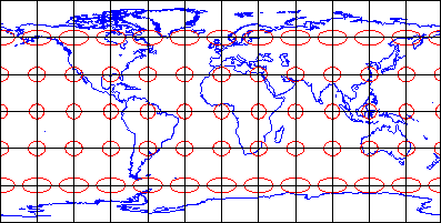
Many types of map projections have been devised to suit particular purposes. No projection allows us to flatten the globe without distorting it, however. Distortion ellipses help us to visualize what type of distortion a map projection has caused, how much distortion has occurred, and where it has occurred. The ellipses show how imaginary circles on the globe are deformed as a result of a particular projection. If no distortion had occurred in the process of projecting the map shown below in Figure 2.29.1, all of the ellipses would be the same size, and circular in shape.

When positions on the graticule are transformed to positions on a projected grid, four types of distortion can occur: distortion of sizes, angles, distances, and directions. Map projections that avoid one or more of these types of distortion are said to preserve certain properties of the globe.

Equivalence

Figure 2.29.1 Equal-Area Distortion

So-called equal-area projections maintain correct proportions in the sizes of areas on the globe and corresponding areas on the projected grid (allowing for differences in scale, of course). Notice that the shapes of the ellipses in the Cylindrical Equal Area projection above (Figure 2.29.1) are distorted, but the areas each one occupies are equivalent. Equal-area projections are preferred for small-scale thematic mapping, especially when map viewers are expected to compare sizes of area features like countries and continents.

Conformality

Figure 2.29.2 Conformal Projection Distortion

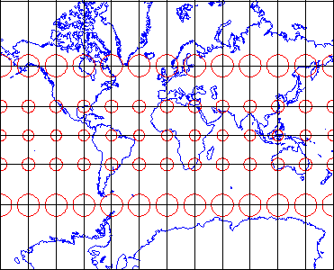
The distortion ellipses plotted on the conformal projection shown above in Figure 2.29.2 vary substantially in size, but are all the same circular shape. The consistent shapes indicate that conformal projections (like this Mercator projection of the world) preserve the fidelity of angle measurements from the globe to the plane. In other words, an angle measured by a land surveyor anywhere on the Earth's surface can be plotted on at its corresponding location on a conformal projection without distortion. This useful property accounts for the fact that conformal projections are almost always used as the basis for large scale surveying and mapping. Among the most widely used conformal projections are the Transverse Mercator, Lambert Conformal Conic, and Polar Stereographic.

Conformality and equivalence are mutually exclusive properties. Whereas equal-area projections distort shapes while preserving fidelity of sizes, conformal projections distort sizes in the process of preserving shapes.

Equidistance

Figure 2.29.3 Equidistant projection distortion

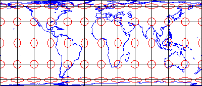
Equidistant map projections allow distances to be measured accurately along straight lines radiating from one or two points only. Notice that ellipses plotted on the Cylindrical Equidistant (Plate Carrée) projection shown above (Figure 2.29.3) vary in both shape and size. The north-south axis of every ellipse is the same length, however. This shows that distances are true-to-scale along every meridian; in other words, the property of equidistance is preserved from the two poles. See chapters 11 and 12 of the online publication Matching the Map Projection to the Need to see how projections can be customized to facilitate distance measurements and to effectively depict ranges and rings of activity.

Azimuthality

Figure 2.29.4 Azimuthal projection distortion

Azimuthal projections preserve directions (azimuths) from one or two points to all other points on the map. See how the ellipses plotted on the gnomonic projection, shown above in Figure 2.29.4, vary in size and shape, but are all oriented toward the center of the projection? In this example, that's the one point at which directions measured on the globe are not distorted on the projected graticule.

Compromise

Figure 2.29.5 Polyconic projection distortion

Some map projections preserve none of the properties described above, but instead seek a compromise that minimizes distortion of all kinds. The example shown above in Figure 2.29.5 is the Polyconic projection, which was used by the U.S. Geological Survey for many years as the basis of its topographic quadrangle map series until it was superceded by the conformal Transverse Mercator. Another example is the Robinson projection, which is often used for small-scale thematic maps of the world.

This textbook is used as a resource in Penn State's Online Geospatial Education online degree and certificate programs. If this topic is interesting to you and you want to learn more about online GIS and GEOINT education at Penn State, check out our Geospatial Education Program Office.

The term "projection" implies that the ball-shaped net of parallels and meridians is transformed by casting its shadow upon some flat, or flattenable, surface. In fact, almost all map projection methods are mathematical equations. The analogy of an optical projection onto a flattenable surface is useful, however, as a means to classify the bewildering variety of projection equations devised over the past two thousand years or more.

Figure 2.30.1 Three types of "flattenable" surfaces to which the graticule can be projected: a plane, a cone, and a cylinder.

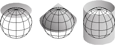
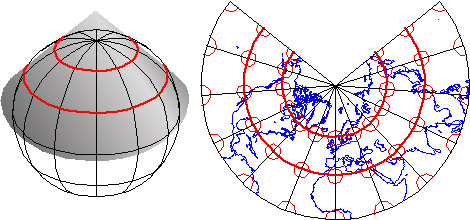
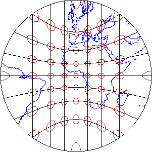
Imagine a model globe that is translucent, and contains a bright light bulb. Imagine the light literally casting shadows of the graticule, and of the shapes of the continents, onto another surface that touches the globe. As you might imagine, the appearance of the projected grid will change quite a lot depending on the type of surface it is projected onto, and how that surface is aligned with the globe. The three surfaces shown above in Figure 2.30.1--the disk-shaped plane, the cone, and the cylinder--represent categories that account for the majority of projection equations that are encoded in GIS software. All three are shown in their normal aspects. The plane often is centered upon a pole. The cone is typically aligned with the globe such that its line of contact (tangency) coincides with a parallel in the mid-latitudes. And the cylinder is frequently positioned tangent to the equator (unless it is rotated 90°, as it is in the Transverse Mercator projection). The following illustrations in Figure 2.30.2 show some of the projected graticules produced by projection equations in each category.

Figure 2.30.2 Four categories of map projections

Cylindric projection equations yield projected graticules with straight meridians and parallels that intersect at right angles. The example shown above at top left in Figure 2.30.2 is a Cylindrical Equidistant (also called Plate Carrée or geographic) in its normal equatorial aspect.

Pseudocylindric projections are variants on cylindrics in which meridians are curved. The result of a Sinusoidal projection is shown above at top right of Figure 2.30.2.

Conic projections yield straight meridians that converge toward a single point at the poles, parallels that form concentric arcs. The example shown above, at bottom left in Figure 2.30.2, is the result of an Albers Conic Equal Area, which is frequently used for thematic mapping of mid latitude regions.

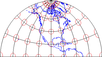
Planar projections also yield meridians that are straight and convergent, but parallels form concentric circles rather than arcs. Planar projections are also called azimuthal because every planar projection preserves the property of azimuthality. The projected graticule shown above at bottom right of Figure 2.30.2 is the result of an Azimuthal Equidistant projection in its normal polar aspect.

Appearances can be deceiving. It's important to remember that the look of a projected graticule depends on several projection parameters, including latitude of projection origin, central meridian, standard line(s), and others. Customized map projections may look entirely different from the archetypes described above.

This textbook is used as a resource in Penn State's Online Geospatial Education online degree and certificate programs. If this topic is interesting to you and you want to learn more about online GIS and GEOINT education at Penn State, check out our Geospatial Education Program Office.

In this chapter, we've explored several connotations of the term scale. Scale is synonymous with scope when it is used to describe the extent of a phenomenon. In this sense, "large scale" means "large area." Specialists in geographic information often use the term differently, however. Map scale refers to the relative sizes of features on a map and of corresponding objects on the ground. In this context, "large scale" implies "small area." Large scale also implies greater detail and greater accuracy, an important point to keep in mind when using maps as sources for GIS databases. Map scale is defined mathematically as the proportion of map distance to ground distance. I hope you are now prepared to use scale equations to calculate map scale.

Scale can also be thought of as a reference system for measurement. Locations on the globe are specified with reference to the geographic coordinate system of latitudes and longitudes. Plane coordinates are often preferred over geographic coordinates because they ease calculations of distance, area, and other quantities. Georeferenced plane coordinate systems like UTM and SPC are established by first flattening the graticule, then superimposing a plane coordinate grid. The mathematical equations used to transform geographic coordinates into plane coordinates are called map projections. Both plane and geographic coordinate system grids are related to approximations of the Earth's size and shape called ellipsoids. Relations between grids and ellipsoids are called horizontal datums.

Horizontal datum is an elusive concept for many GIS practitioners. It is relatively easy to visualize a horizontal datum in the context of unprojected geographic coordinates. Simply drape the latitude and longitude grid over an ellipsoid and there's your horizontal datum. It is harder to think about datum in the context of a projected coordinate grid like UTM and SPC, however. Think of it this way: First drape the latitude and longitude grid on an ellipsoid. Then project that grid to a 2-D plane surface. Then, superimpose a rectangular grid of eastings and northings over the projection, using control points to georegister the grids. There you have it--a projected coordinate grid based upon a horizontal datum.

Numerous coordinate systems, datums, and map projections are in use around the world. Because we often need to combine georeferenced data from various sources, GIS professionals need to be able to georegister two or more data sets that are based upon different coordinate systems, datums, and/or projections. Transformations, including coordinate transformations, datum transformations, and map projections, are the mathematical procedures used to bring diverse data into alignment. Characteristics of the coordinate systems, datums, and projections considered in this text are outlined in the following tables.

Coordinate systems referenced in this text

(many other national and local systems are in use)

Datums referenced in this text

(many other national and local systems are in use)

Map projections referenced in this text

(many other national and local systems are in use)

Compiled from Snyder, 1997

This textbook is used as a resource in Penn State's Online Geospatial Education online degree and certificate programs. If this topic is interesting to you and you want to learn more about online GIS and GEOINT education at Penn State, check out our Geospatial Education Program Office.