Chapter 9: Integrating Geographic Data
1. Overview
Geographic data are expensive to produce and maintain. Data often accounts for the lion's share of the cost of building and running geographic information systems. The expense of GIS is justifiable when it gives people the information they need to make wise choices in the face of complex problems. In this chapter, we'll consider one such problem: the search for suitable and acceptable sites for low level radioactive waste disposal facilities. Two case studies will demonstrate that GIS is very useful indeed for assimilating the many site suitability criteria that must be taken into account, provided that the necessary data can be assembled in a single, integrated system. The case studies will allow us to compare vector and raster approaches to site selection problems.
The ability to integrate diverse geographic data is a hallmark of mature GIS software. The know-how required to accomplish data integration is also the mark of a truly knowledgeable GIS user. What knowledgeable users also recognize, however, is that while GIS technology is well suited to answering certain well-defined questions, it often cannot help resolve crucial conflicts between private and public interests. The objective of this final, brief chapter is to consider the challenges involved in using GIS to address a complex problem that has both environmental and social dimensions.
Objectives
Students who successfully complete Chapter 9 should be able to:
- recognize the characteristics of geographic data that must be taken into account to overlay multiple data layers;
- compare and contrast vector and raster approaches to site suitability studies;
- gave realistic expectations about what geographic data analysis can achieve.
"Try This!" Activities
Take a minute to complete any of the Try This activities that you encounter throughout the chapter. These are fun, thought provoking exercises to help you better understand the ideas presented in the chapter.
2. Context
This section sets a context for two case studies that follow. First, I will briefly define low-level radioactive waste (LLRW). Then I discuss the legislation that mandated construction of a dozen or more regional LLRW disposal facilities in the U.S. Finally, I will reflect briefly on how the capability of geographic information systems to integrate multiple data "layers" is useful for siting problems like the ones posed by LLRW.
3. Low Level Radioactive Waste
According to the U.S. Nuclear Regulatory Commission (2004), LLRW consists of discarded items that have become contaminated with radioactive material or have become radioactive through exposure to neutron radiation. Trash, protective clothing, and used laboratory glassware make up all but about 3 percent of LLRW. These "Class A" wastes remain hazardous less than 100 years. "Class B" wastes, consisting of water purification filters and ion exchange resins used to clean contaminated water at nuclear power plants, remain hazardous up to 300 years. "Class C" wastes, such as metal parts of decommissioned nuclear reactors, constitute less than 1 percent of all LLRW, but remain dangerous for up to 500 years.
The danger of exposure to LLRW varies widely according to the types and concentration of radioactive material contained in the waste. Low level waste containing some radioactive materials used in medical research, for example, is not particularly hazardous unless inhaled or consumed, and a person can stand near it without shielding. On the other hand, exposure to LLRW contaminated by processing water at a reactor can lead to death or an increased risk of cancer (U.S. Nuclear Regulatory Commission, n.d.).
Figure 9.4.1 shows a bar graph and a pie chart that appear here in table form.Note that Volumes are rounded to the nearest thousand cubic feet and percentages are rounded to the nearest tenth of a percent.
| Year | Volume (Thousands of Cubic Feet) |
|---|---|
| 1985 | 2681 |
| 1986 | 1805 |
| 1987 | 1842 |
| 1988 | 1428 |
| 1989 | 1626 |
| 1990 | 1143 |
| 1991 | 1369 |
| 1992 | 1743 |
| 1993 | 792 |
| 1994 | 859 |
| 1995 | 690 |
| 1996 | 422 |
| 1997 | 319 |
| 1998 | 1419 |
| Facility Name | Cubic Feet / Percentage |
|---|---|
| Envirocare | 1080K / 76.1% |
| Barnwell | 194K / 13.7% |
| Richland | 145K / 10.2% |
Hundreds of nuclear facilities across the country produce LLRW, but only a very few disposal sites are currently willing to store it. Disposal facilities at Clive, Utah; Barnwell, South Carolina; and Richland, Washington accepted over 4,000,000 cubic feet of LLRW in both 2005 and 2006, up from 1,419,000 cubic feet in 1998. By 2008, the volume had dropped to just over 2,000,000 cubic feet (U.S. Nuclear Regulatory Commission, 2011a). Sources include nuclear reactors, industrial users, government sources (other than nuclear weapons sites), and academic and medical facilities. (We have a small nuclear reactor here at Penn State that is used by students in graduate and undergraduate nuclear engineering classes.)
4. Siting LLRW Storage Facilities
The U.S. Congress passed the Low-Level Radioactive Waste Policy Act in 1980. As amended in 1985, the Act made states responsible for disposing of the LLRW they produce. States were encouraged to form regional "compacts" to share the costs of locating, constructing, and maintaining LLRW disposal facilities. The intent of the legislation was to avoid the very situation that has since come to pass, that the entire country would become dependent on a very few disposal facilities.

State government agencies and the consultants they hire to help select suitable sites assume that few if any municipalities would volunteer to host a LLRW disposal facility. They prepare for worst-case scenarios in which states would be forced to exercise their right of eminent domain to purchase suitable properties without the consent of landowners or their neighbors. GIS seems to offer an impartial, scientific, and therefore defensible approach to the problem. As Mark Monmonier has written, "[w]e have to put the damned thing somewhere, the planners argue, and a formal system of map analysis offers an 'objective,' logical method for evaluating plausible locations" (Monmonier, 1995, p. 220). As we discussed in our very first chapter, site selection problems pose a geographic question that geographic information systems are well suited to address, namely, which locations have attributes that satisfy all suitability criteria?
5. Map Overlay Concept
Environmental scientists and engineers consider many geological, climatological, hydrological, and surface and subsurface land use criteria to determine whether a plot of land is suitable or unsuitable for a LLRW facility. Each criterion can be represented with geographic data, and visualized as a thematic map. In theory, the site selection problem is as simple as compiling onto a single map all the disqualified areas on the individual maps, and then choosing among whatever qualified locations remain. In practice, of course, it is not so simple.
There is nothing new about superimposing multiple thematic maps to reveal optimal locations. One of the earliest and most eloquent descriptions of the process was written by Ian McHarg, a landscape architect and planner, in his influential book Design With Nature. In a passage describing the process he and his colleagues used to determine the least destructive route for a new roadway, McHarg (1971) wrote:
...let us map physiographic factors so that the darker the tone, the greater the cost. Let us similarly map social values so that the darker the tone, the higher the value. Let us make the maps transparent. When these are superimposed, the least-social-cost areas are revealed by the lightest tone. (p. 34).
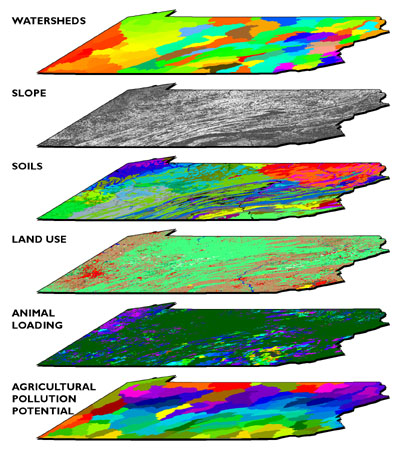
As you probably know, this process has become known as map overlay. Storing digital data in multiple "layers" is not unique to GIS, of course; computer-aided design (CAD) packages and even spreadsheets also support layering. What's unique about GIS, and important about map overlay, is its ability to generate a new data layer as a product of existing layers. In the example illustrated below, for example, analysts at Penn State's Environmental Resources Research Institute estimated the agricultural pollution potential of every major watershed in the state by overlaying watershed boundaries, the slope of the terrain (calculated from USGS DEMs), soil types (from U.S. Soil Conservation Service data), land use patterns (from the USGS LULC data), and animal loading (livestock wastes estimated from the U.S. Census Bureau's Census of Agriculture).
As illustrated below, map overlay can be implemented in either vector or raster systems. In the vector case, often referred to as polygon overlay, the intersection of two or more data layers produces new features (polygons). Attributes (symbolized as colors in the illustration) of intersecting polygons are combined. The raster implementation (known as grid overlay) combines attributes within grid cells that align exactly. Misaligned grids must be resampled to common formats.
Polygon and grid overlay procedures produce useful information only if they are performed on data layers that are properly georegistered. Data layers must be referenced to the same coordinate system (e.g., the same UTM and SPC zones), the same map projection (if any), and the same datum (horizontal and vertical, based upon the same reference ellipsoid). Furthermore, locations must be specified with coordinates that share the same unit of measure.
6. Pennsylvania Case Study
In response to the LLRW Policy Act, Pennsylvania entered into an "Appalachian Compact" with the states of Delaware, Maryland, and West Virginia to share the costs of siting, building, and operating a LLRW storage facility. Together, these states generated about 10 percent of the total volume of LLRW then produced in the United States. Pennsylvania, which generated about 70 percent of the total produced by the Appalachian Compact, agreed to host the disposal site.
In 1990, the Pennsylvania Department of Environmental Protection commissioned Chem-Nuclear Systems Incorporated (CNSI) to identify three potentially suitable sites to accommodate two to three truckloads of LLRW per day for 30 years. CNSI, the operator of the Barnwell South Carolina site, would also operate the Pennsylvania site for profit.
CNSI's plan called for storing LLRW in 55-gallon drums encased in concrete, buried in clay, surrounded by a polyethylene membrane. The disposal facilities, along with support and administration buildings and a visitors center, would occupy about 50 acres in the center of a 500-acre site. (Can you imagine a family outing to the Visitors Center of a LLRW disposal facility?) The remaining 450 acres would be reserved for a 500 to 1000 foot wide buffer zone.
The three-stage siting process agreed to by CNSI and the Pennsylvania Department of Environmental Protection corresponded to three scales of analysis: statewide, regional, and local. All three stages relied on vector geographic data integrated within a GIS.
7. Vector Approach
CNSI and its subcontractors adopted a vector approach for its GIS-based site selection process. When the process began in 1990, far less geographic data was available in digital form than it is today. Most of the necessary data was available only as paper maps, which had to be converted to digital form. In one of its interim reports, CNSI described two digitizing procedures used, "digitizing" and "scanning." Here's how it described "digitizing:"
In the digitizing process, a GIS operator uses a hand-held device, known as a cursor, to trace the boundaries of selected disqualifying features while the source map is attached to a digitizing table. The digitizing table contains a fine grid of sensitive wire imbedded within the table top. This grid allows the attached computer to detect the position of the cursor so that the system can build an electronic map during the tracing. In this project, source maps and GIS-produced maps were compared to ensure that the information was transferred accurately. (Chem Nuclear Systems, 1993, p. 8).
One aspect overlooked in the CNSI description is that operators must encode the attributes of features as well as their locations. Some of you know all too well that tablet digitizing (illustrated at left in Figure 9.8.1, below) is an extraordinarily tedious task, so onerous that even student interns resent it. One wag here at Penn State suggested that the acronym "GIS" actually stands for "Getting it (the data) In Stinks." You can substitute your own "S" word if you wish.
Compared to the drudgery of tablet digitizing, electronically scanning paper maps seems simple and efficient. Here's how CNSI describes it:
The scanning process is more automated than the digitizing process. Scanning is similar to photocopying, but instead of making a paper copy, the scanning device creates an electronic copy of the source map and stores the information in a computer record. This computer record contains a complete electronic picture (image) of the map and includes shading, symbols, boundary lines, and text. A GIS operator can select the appropriate feature boundaries from such a record. Scanning is useful when maps have very complex boundaries lines that can not be easily traced. (Chem Nuclear Systems, Inc., 1993, p. 8)
I hope you noticed that CNSI's description glosses over the distinction between raster and vector data. If scanning is really as easy as they suggest, why would anyone ever tablet-digitize anything? In fact, it is not quite so simple to "select the appropriate feature boundaries" from a raster file, which is analogous to a remotely sensed image. The scanned maps had to be transformed from pixels to vector features using a semi-automated procedure called raster to vector conversion, otherwise known as "vectorization." Time-consuming manual editing is required to eliminate unwanted features (like vectorized text), correct digital features that were erroneously attached or combined, and to identify the features by encoding their attributes in a database.
In either the vector or raster case, if the coordinate system, projection, and datums of the original paper map were not well defined, the content of the map first had to be redrawn, by hand, onto another map whose characteristics are known.
8. Stage One: Statewide Screening
CNSI considered several geological, hydrological, surface and subsurface land use criteria in the first stage of its LLRW siting process. [View a table that lists all the Stage One criteria.] CNSI's GIS subcontractors created separate digital map layers for every criterion. Sources and procedures used to create three of the map layers are discussed briefly below.
One of the geological criteria considered was carbonate lithology. Limestone and other carbonate rocks are permeable. Permeable bedrock increases the likelihood of groundwater contamination in the event of a LLRW leak. Areas with carbonate rock outcrops were therefore disqualified during the first stage of the screening process. Boundaries of disqualified areas were digitized from the 1:250,000-scale Geologic Map of Pennsylvania (1980). What concerns would you have about data quality, given a 1:250,000-scale source map?
Analysts needed to make sure that the LLRW disposal facility would never be inundated with water in the event of a coastal flood or a rise in sea level. To determine disqualified areas, CNSI's subcontractors relied upon the Federal Emergency Management Agency's Flood Insurance Rate Maps (FIRMs). The maps were not available in digital form at the time and did not include complete metadata. According to the CNSI interim report, "[t]he 100-year flood plains shown on maps obtained from FEMA ... were transferred to USGS 7.5-minute quad sheet maps. The 100-year floodplain boundaries were digitized into the GIS from the 7.5-minute quad sheet maps." (Chem Nuclear Systems, 1991, p. 11) Why would the contractors go to the trouble of redrawing the floodplain boundaries onto topographic maps prior to digitizing?
Areas designated as "exceptional value watersheds" were also disqualified during Stage One. Pennsylvania legislation protected 96 streams. Twenty-nine additional streams were added during the site screening process. "The watersheds were delineated on county [1:50,000 or 1:100,000-scale topographic] maps by following the appropriate contour lines. Once delineated, the EV stream and its associated watershed were digitized into the GIS." (Chem Nuclear Systems, 1991, p. 12) What digital data sets could have been used to delineate the watersheds automatically, had the data been available?
After all the Stage One maps were digitized, georegistered, and overlayed, approximately 23 percent of the state's land area was disqualified.
9. Stage Two: Regional Screening
CNSI considered additional disqualification criteria during the second, "regional" stage of the LLRW siting process. [View a table that lists all the Stage Two criteria.] Some of the Stage Two criteria had already been considered during Stage One, but were now reassessed in light of more detailed data compiled from larger-scale sources. In its interim report, CNSI had this to say about the composite disqualification map shown below:
When all the information was entered in to Stage Two database, the GIS was used to draw the maps showing the disqualified land areas. ... The map shows both additions/refinements to the Stage One disqualifying features and those additional disqualifying features examined during Stage Two. (Chem Nuclear Systems, 1993, p. 19)
CNSI added this disclaimer:
The Stage Two Disqualifying maps found in Appendix A depict information at a scale of 1:1.5 million. At this scale, one inch on the map represents 24 miles, or one mile is represented on the map by approximately four one-hundreds of an inch. A square 500-acre area measures less than one mile on a side. Printing of such fine detail on the 11" × 17" disqualifying maps was not possible, therefore, it is possible that small areas of sufficient size for the LLRW disposal facility site may exist within regions that appear disqualified on the attached maps. [Emphasis in the original document] The detailed boundary information for these small areas is retained within the GIS even though they are not visually illustrated on the maps. (Chem Nuclear Systems, 1993, p. 20)
As I mentioned back in Chapter 2, CNSI representatives took some heat about the map scale problem in public hearings. Residents took little solace in the assertion that the data in the GIS were more truthful than the data depicted on the map.
10. Stage Three: Local Disqualification
Many more criteria were considered in Stage Three. [View a table that lists all the Stage Three criteria.] At the completion of the third stage, roughly 75 percent of the state's land area had been disqualified.
One of the new criteria introduced in Stage Three was slope. Analysts were concerned that precipitation runoff, which increases as slope increases, might increase the risk of surface water contamination should the LLRW facility spring a leak. CNSI's interim report (1994a) states that "[t]he disposal unit area which constitutes approximately 50 acres ... may not be located where there are slopes greater than 15 percent as mapped on U.S. Geological Survey (USGS) 7.5-minute quadrangles utilizing a scale of 1:24,000 ..." (p. 9).
Slope is change in terrain elevation over a given horizontal distance. It is often expressed as a percentage. A 15 percent slope changes at a rate of 15 feet of elevation for every 100 feet of horizontal distance. Slope can be measured directly on topographic maps. The closer the spacing of elevation contours, the greater the slope. CNSI's GIS subcontractors were able to identify areas with excessive slope on topographic maps using plastic templates called "land slope indicators" that showed the maximum allowable contour spacing.
Fortunately for the subcontractors, 7.5-minute USGS DEMs were available for 85 percent of the state (they're all available now). Several algorithms have been developed to calculate slope at each grid point of a DEM. As described in chapter 7, the simplest algorithm calculates slope at a grid point as a function of the elevations of the eight points that surround it to the north, northeast, east, southeast, and so on. CNSI's subcontractors used GIS software that incorporated such an algorithm to identify all grid points whose slopes were greater than 15 percent. The areas represented by these grid points were then made into a new digital map layer.
Try This!
You can create a slope map of the Bushkill PA quadrangle with Global Mapper (dlgv32 Pro) software.
- Launch Global Mapper.
- Open the file "bushkill_pa.dem" that you downloaded earlier (either the 10-meter or 30-meter version).
- Change from the default "HSV" shader to the "Slope" shader.
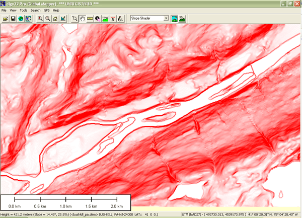
By default, pixels with 0 percent slope are lightest, and pixels with 30 percent slope or more are darkest. You can adjust this at Tools > Configure > Shader Options.
Notice that the slope symbolization does not change even as you change the vertical exaggeration of the DEM (Tools > Configure > Vertical Options).
11. Buffering
Several of the disqualification criteria involve buffer zones. For example, one disqualifying criterion states that "[t]he area within 1/2 mile of an existing important wetland ... is disqualified." Another states that "disposal sites may not be located within 1/2 mile of a well or spring which is used as a public water supply." (Chem-Nuclear Systems, 1994b). As I mentioned in the first chapter (and as you may know from experience), buffering is a GIS procedure by which zones of specified radius or width are defined around selected vector features or raster grid cells.
Like map overlay, buffering has been implemented in both vector and raster systems. The vector implementation involves expanding a selected feature or features, or producing new surrounding features (polygons). The raster implementation accomplishes the same thing, except that buffers consist of sets of pixels rather than discrete features.
12. New York Case Study
Like Pennsylvania, the State of New York was compelled by the LLRW Policy Act to dispose of its waste within its own borders. New York also turned to GIS in the hope of finding a systematic and objective means of determining an optimal site. Instead of the vector approach used by its neighbor, however, New York opted for a raster framework.
Mark Monmonier, a professor of geography at Syracuse University (and a Penn State alumnus), has written that the list of siting criteria assembled by the New York Department of Environmental Conservation (DEC) was "an astute mixture of common sense, sound environmental science, and interest-group politics" (1995, p. 226). Source data included maps and attribute data produced by the U.S. Census Bureau, the New York Department of Transportation, and the DEC itself, among others. The New York LLRW Siting Commission overlaid the digitized source maps with a grid composed of cells that corresponded to one square mile (640 acres; slightly larger than the 500 acres required for a disposal site) on the ground. As illustrated above, the Siting Commission's GIS subcontractors then assigned each of the 47,224 grid cells a "favorability" score for each criterion. The process was systematic, but hardly objective, since the scores reflected social values (to borrow the term used by McHarg).
To acknowledge the fact that some criteria were more important than others, the Siting Commission weighted the scores in each data layer by multiplying them all by a constant factor. Like the original integer scores, the weighting factors were a negotiated product of consensus, not of objective measurement. Finally, the commission produced a single set of composite scores by summing the scores of each raster cell through all the data layers. A composite favorability map could then be produced from the composite scores. All that remained was for the public to embrace the result.
13. Outcomes
To date, neither Pennsylvania nor New York has built an LLRW disposal facility. Both states gave up on their unpopular sitting programs shortly after Republicans replaced Democrats in the 1994 gubernatorial elections.
The New York process was derailed when angry residents challenged proposed sites on account of inaccuracies discovered in the state's GIS data, and because of the state's failure to make the data accessible for citizen review in accordance with the Freedom of Information Act (Monmonier, 1995).
Pennsylvania's $37 million siting effort succeeded in disqualifying more than three-quarters of the state's land area but failed to recommend any qualified 500-acre sites. With the volume of its LLRW decreasing, and the Barnwell South Carolina facility still willing to accept Pennsylvania's waste shipments, the search was suspended "indefinitely" in 1998.
To fulfill its obligations under the LLRW Policy Act, Pennsylvania has initiated a "Community Partnering Plan" that solicits volunteer communities to host a LLRW disposal facility in return for jobs, construction revenues, shares of revenues generated by user fees, property taxes, scholarships, and other benefits. The plan has this to say about the GIS site selection process that preceded it: "The previous approach had been to impose the state's will on a municipality by using a screening process based primarily on technical criteria. In contrast, the Community Partnering Plan is voluntary." (Chem Nuclear Systems, 1996, p. 3)
The New York and Pennsylvania state governments turned to GIS because it offered an impartial and scientific means to locate a facility that nobody wanted in their backyard. Concerned residents criticized the GIS approach as impersonal and technocratic. There is truth to both points of view. Specialists in geographic information need to understand that while GIS can be effective in answering certain well-defined questions, it does not ease the problem of resolving conflicts between private and public interests.
Meanwhile, a Democrat replaced a Republican as governor of South Carolina in 1998. The new governor warned that the Barnwell facility might not continue to accept out-of-state LLRW. "We don't want to be labeled as the dumping ground for the entire country," his spokesperson said (Associated Press, 1998).
No volunteer municipality has yet come forward in response to Pennsylvania's Community Partnering Plan. If the South Carolina facility does stop accepting Pennsylvania's LLRW shipments, and if no LLRW disposal facility is built within the state's borders, then nuclear power plants, hospitals, laboratories, and other facilities may be forced to store LLRW on site. It will be interesting to see if the GIS approach to site selection is resumed as a last resort, or if the state will continue to up the ante in its attempts to attract volunteers, in the hope that every municipality has its price. If and when a volunteer community does come forward, detailed geographic data will be produced, integrated, and analyzed to make sure that the proposed site is suitable, after all.
Try This!
To find out about LLRW-related activities where you live, use your favorite search engine to search the Web on "Low-Level Radioactive Waste [your state or area of interest]". If GIS is involved in your state's LLRW disposal facility site selection process, your state agency that is concerned with environmental affairs is likely to be involved.
14. Conclusion
Site selection projects like the ones discussed in this chapter require the integration of diverse geographic data. The ability to integrate and analyze data organized in multiple thematic layers is a hallmark of geographic information systems. To contribute to GIS analyses like these, you need to be both a knowledgeable and skillful GIS user. The objective of this text, and the associated Penn State course, has been to help you become more knowledgeable about geographic data.
Knowledgeable users are well versed in the properties of geographic data that need to be taken into account to make data integration possible. Knowledgeable users understand the distinction between vector and raster data, and know something about how features, topological relationships among features, attributes, and time can be represented within the two approaches. Knowledgeable users understand that in order for geographic data to be organized and analyzed as layers, the data must be both orthorectified and georegistered. Knowledgeable users look out for differences in coordinate systems, map projections, and datums that can confound efforts to georegister data layers. Knowledgeable users know that the information needed to register data layers is found in metadata.
Knowledgeable users understand that all geographic data are generalized, and that the level of detail preserved depends upon the scale and resolution at which the data were originally produced. Knowledgeable users are prepared to convince their bosses that small-scale, low resolution data should not be used for large-scale analyses that require high resolution results. Knowledgeable users never forget that the composition of the Earth's surface is constantly changing, and that unlike fine wine, the quality of geographic data does not improve over time.
Knowledgeable users are familiar with the characteristics of the "framework" data that make up the U.S. National Spatial Data Infrastructure, and are able to determine whether these data are available for a particular location. Knowledgeable users recognize situations in which existing data are inadequate, and when new data must be produced. They are familiar enough with geographic information technologies such as GPS, aerial imaging, and satellite remote sensing that they can judge which technology is best suited to a particular mapping problem.
And knowledgeable users know what kinds of questions GIS is, and is not, suited to answer.