Chapters 6 and 7 consider the origins and characteristics of the framework data themes that make up the United States' proposed National Spatial Data Infrastructure (NSDI). The seven themes include geodetic control, orthoimagery, elevation, transportation, hydrography, government units (administrative boundaries), and cadastral (property boundaries). Most framework data, like the printed topographic maps that preceded them, are derived directly or indirectly from aerial imagery. Chapter 6 introduces the field of photogrammetry, which is concerned with the production of geographic data from aerial imagery. The chapter begins by considering the nature and status of the U.S. NSDI in comparison with other national mapping programs. It considers the origins and characteristics of the geodetic control and orthoimagery themes. The remaining five themes are the subject of Chapter 7.

Objectives

Students who successfully complete Chapter 6 should be able to:

1. explain how the distribution of authority for mapping and land title registration among various levels of government affects the availability of framework data;
2. describe how topographic data are compiled from aerial imagery;
3. explain the difference between a vertical aerial photograph and an orthoimage;
4. list and describe characteristics and status of the USGS National Map; and
5. discuss the relationship between the National Map and the NSDI framework.

"Try This!" Activities

Take a minute to complete any of the Try This activities that you encounter throughout the chapter. These are fun, thought provoking exercises to help you better understand the ideas presented in the chapter.

This textbook is used as a resource in Penn State's Online Geospatial Education online degree and certificate programs. If this topic is interesting to you and you want to learn more about online GIS and GEOINT education at Penn State, check out our Geospatial Education Program Office.

In 1998, Ian Masser published a comparative study of the national geographic information strategies of four developed countries: Britain (England and Wales), the Netherlands, Australia, and the United States. Masser built upon earlier work which found that countries with relatively low levels of digital data availability and GIS diffusion also tended to be countries where there had been a fragmentation of data sources in the absence of central or local government coordination” (p. ix). Comparing his four case studies in relation to the seven framework themes identified for the U.S. NSDI, Masser found considerable differences in data availability, pricing, and intellectual property protections. Differences in availability of core data, he found, are explained by the ways in which responsibilities for mapping and for land titles registration are distributed among national, state, and local governments in each country.
The following table summarizes those distributions of responsibilities.

Masser's analysis helps to explain what geospatial professionals in the U.S. have known all along -- that the coverage of framework data in the U.S. is incomplete or fragmented because thousands of local governments are responsible for large-scale mapping and land titles registration, and because these activities tend to be poorly coordinated. In contrast, core data coverage is more or less complete in Australia, the Netherlands, and Britain, where central and state governments have authority over large-scale mapping and land-titles registration.

Other differences among the four countries relate to fees charged by governments to use the geographic and statistical data they produce, as well as the copyright protections they assert over the data. U.S. federal government agencies, Masser notes, differ from their counterparts by charging no more than the cost of reproducing their data in forms suitable for delivery to customers. State and local government policies in the U.S. vary considerably, however. Longstanding debates persist in the U.S. about the viability and ethics of recouping costs associated with public data.

The U.S. also differs starkly from Britain and Australia in regards to copyright protection. Most data published by the U.S. Geological Survey or U.S. Census Bureau resides in the public domain and may be used without restriction. U.K. Ordnance Survey data, by contrast, is protected by Crown copyright, and is available for use by others for fees and under the terms of restrictive licensing agreements. One consequence of the federal government’s decision to release its geospatial data to the public domain, some have argued, was the early emergence of a vigorous geospatial industry in the U.S.

This textbook is used as a resource in Penn State's Online Geospatial Education online degree and certificate programs. If this topic is interesting to you and you want to learn more about online GIS and GEOINT education at Penn State, check out our Geospatial Education Program Office.

Since the eighteenth century, the preparation of a detailed basic reference map has been recognized by the governments of most countries as fundamental for the delimitation of their territory, for underpinning their national defense and for management of their resources (Parry, 1987).

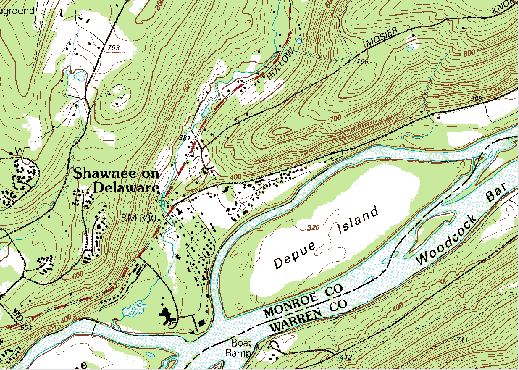
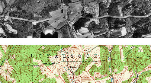
Specialists in geographic information recognize two broad functional classes of maps: reference maps and thematic maps. As you recall from Chapter 3, a thematic map is usually made with one particular purpose in mind. Often, the intent is to make a point about the spatial pattern of a single phenomenon. Reference maps, on the other hand, are designed to serve many different purposes. Like a reference book, such as a dictionary, encyclopedia, or gazetteer, reference maps help people look up facts. Common uses of reference maps include locating place names and features, estimating distances, directions, and areas, and determining preferred routes from starting points to a destination. Reference maps are also used as base maps upon which additional geographic data can be compiled. Because reference maps serve various uses, they typically include a greater number and variety of symbols and names than thematic maps. The portion of the United States Geological Survey (USGS) topographic map shown below is a good example.

Figure 6.4.1 A typical reference map. A portion of a USGS topographic quadrangle map.

Credit: USGS, 1971

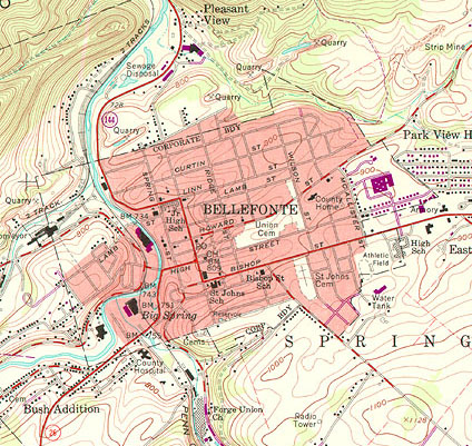
The term topography derives from the Greek topographein, "to describe a place." Topographic maps show, and name, many of the visible characteristics of the landscape, as well as political and administrative boundaries. Topographic map series provide base maps of uniform scale, content, and accuracy (more or less) for entire territories. Many national governments include agencies responsible for developing and maintaining topographic map series for a variety of uses, from natural resource management to national defense. Affluent countries, countries with especially valuable natural resources, and countries with large or unusually active militaries tend to be mapped more completely than others.

The systematic mapping of the entire U.S. began in 1879 when the U.S. Geological Survey (USGS) was established. Over the next century, USGS and its partners created topographic map series at several scales, including 1:250,000, 1:100,000, 1:63,360, and 1:24,000. The diagram below illustrates the relative extents of the different map series. Since much of today’s digital map data was digitized from these topographic maps, one of the challenges of creating continuous digital coverage of the entire U.S. is to seam together all of these separate map sheets.

Figure 6.4.2 Relative extents of the several USGS quadrangle map series.

Credit: Thompson, 1988

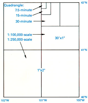
Map sheets in the 1:24,000-scale series are known as quadrangles or simply quads. A quadrangle is a four-sided polygon. Although each 1:24,000 quad covers 7.5 minutes longitude by 7.5 minutes latitude, their shapes and area coverage vary. The area covered by the 7.5-minute maps varies from 49 to 71 square miles (126 to 183 square kilometers) because the length of a degree of longitude varies with latitude.

Figure 6.4.3 Topographer compiling topographic map using a plane table and alidade.

Credit: NOAA, 2007

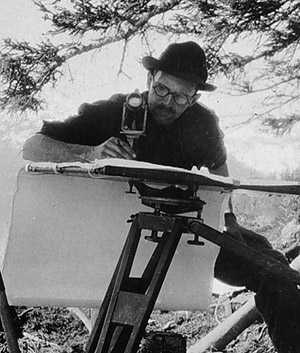
Through the 1940s, topographers in the field compiled by hand the data depicted on topographic maps. Anson (2002) recalls being outfitted with a 14 inch x 14-inch tracing table and tripod, plus an alidade [a 12 inch telescope mounted on a brass ruler], a 13 foot folding stadia rod, a machete, and a canteen... (p. 1). Teams of topographers sketched streams, shorelines, and other water features; roads, structures, and other features of the built environment; elevation contours, and many other features. To ensure geometric accuracy, their sketches were based upon geodetic control provided by land surveyors, as well as positions and spot elevations they surveyed themselves using alidades and rods. Depending on the terrain, a single 7.5-minute quad sheet might take weeks or months to compile. In the 1950s, however, photogrammetric methods involving stereoplotters that permitted topographers to make accurate stereoscopic measurements directly from overlapping pairs of aerial photographs provided a viable and more efficient alternative to field mapping. We’ll consider photogrammetry in greater detail later on in this chapter.

By 1992, the series of over 53,000 separate quadrangle maps covering the lower 48 states, Hawaii, and U.S. territories at 1:24,000 scale was completed, at an estimated total cost of $2 billion. However, by the end of the century, the average age of 7.5-minute quadrangles was over 20 years, and federal budget appropriations limited revisions to only 1,500 quads a year (Moore, 2000). As landscape change has exceeded revisions in many areas of the U.S., the USGS topographic map series has become legacy data outdated in terms of format as well as content.

This textbook is used as a resource in Penn State's Online Geospatial Education online degree and certificate programs. If this topic is interesting to you and you want to learn more about online GIS and GEOINT education at Penn State, check out our Geospatial Education Program Office.

Errors and uncertainty are inherent in geographic data. Despite the best efforts of the USGS Mapping Division and its contractors, topographic maps include features that are out of place, features that are named or symbolized incorrectly, and features that are out of date.

As discussed in Chapter 2, the locational accuracy of spatial features encoded in USGS topographic maps and data are guaranteed to conform to National Map Accuracy Standards. The standard for topographic maps state that horizontal positions of 90 percent of the well-defined points tested will occur within 0.02 inches (map distance) of their actual positions. Similarly, the vertical positions of 90 percent of well-defined points tested are to be true to within one-half of the contour interval. Both standards, remember, are scale-dependent.

Objective standards do not exist for the accuracy of attributes associated with geographic features. Attribute errors certainly do occur, however. A chronicler of the national mapping program (Thompson, 1988, p. 106) recalls a worried user who complained to USGS that "My faith in map accuracy received a jolt when I noted that on the map the borough water reservoir is shown as a sewage treatment plant."

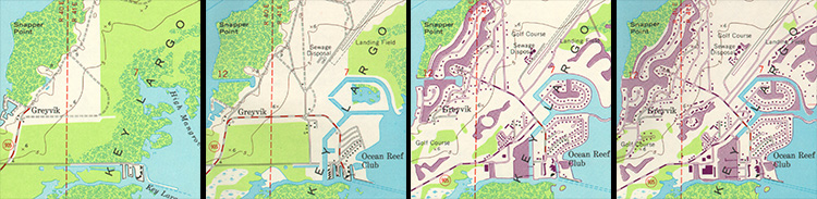
The passage of time is perhaps the most troublesome source of errors on topographic maps. As mentioned in the previous page, the average age of USGS topographic maps is over 20 years. Geographic data quickly lose value (except for historical analyses) unless they are continually revised. The sequence of map fragments below show how frequently revisions were required between 1949 and 1973 for the quad that covers Key Largo, Florida. Revisions are based primarily on geographic data produced by aerial photography.

Figure 6.5.1 Geographic data quickly lose value if they are not kept up to date. Shown here are portions of topographic maps of Key Largo FL in 1949, 1956, 1969, and 1973.

Credit: Adapted from Thompson, 1988

This textbook is used as a resource in Penn State's Online Geospatial Education online degree and certificate programs. If this topic is interesting to you and you want to learn more about online GIS and GEOINT education at Penn State, check out our Geospatial Education Program Office.

Many digital data products have been derived from the USGS topographic map series. The simplest of such products are Digital Raster Graphics (DRGs). DRGs are scanned raster images of USGS 1:24,000 topographic maps. DRGs are useful as backdrops over which other digital data may be superimposed. For example, the accuracy of a vector file containing lines that represent lakes, rivers, and streams could be checked for completeness and accuracy by plotting it over a DRG.

Figure 6.6.1 Portion of a Digital Raster Graphic (DRG) for Bushkill, PA.

DRGs are created by scanning paper maps at 250 pixels per inch resolution. Since at 1:24,000 1 inch on the map represents 2,000 feet on the ground, each DRG pixel corresponds to an area about 8 feet (2.4 meters) on a side. Each pixel is associated with a single attribute: a number from 0 to 12. The numbers stand for the 13 standard DRG colors.

Figure 6.6.2 Magnified portion of a Digital Raster Graphic (DRG) for Bushkill, PA

Like the paper maps from which they are scanned, DRGs comply with National Map Accuracy Standards. A subset of the more than 50,000 DRGs that cover the lower 48 states have been sampled and tested for completeness and positional accuracy.

DRGs conform to the Universal Transverse Mercator projection used in the local UTM zone. The scanned images are transformed to the UTM projection by matching the positions of 16 control points. Like topographic quadrangle maps, all DRGs within one UTM zone can be fit together to form a mosaic after the map "collars" are removed.

Check out USA Topo Maps, a web map that provides a seamless digital compilation of USGS topographic maps for the entire United States. This is a multi-scale web map hosted in ArcGIS Online. As you zoom in, you'll view different scales of digitized topographic maps. The largest-scale images are built from USGS DRGs.

This textbook is used as a resource in Penn State's Online Geospatial Education online degree and certificate programs. If this topic is interesting to you and you want to learn more about online GIS and GEOINT education at Penn State, check out our Geospatial Education Program Office.

Even before the USGS completed its nationwide 7.5-minute quadrangle series, the U.S. federal government had begun to rethink and reorganize its national mapping program. In 1990, the U.S. Office of Management and Budget issued Circular A-16, which established the Federal Geographic Data Committee (FGDC) as the interagency coordinating body responsible for facilitating cooperation among federal agencies whose missions include producing and using geospatial data. FGDC is chaired by the Department of Interior, and is administered by USGS.

In 1994, President Bill Clinton’s Executive Order 12906 charged the FGDC with coordinating the efforts of government agencies and private sector firms leading to a National Spatial Data Infrastructure (NSDI). The Order defined NSDI as "the technology, policies, standards and human resources necessary to acquire, process, store, distribute, and improve utilization of geospatial data" (White House, 1994). It called upon FGDC to establish a National Geospatial Data Clearinghouse, ordered federal agencies to make their geospatial data products available to the public through the Clearinghouse, and required them to document data in a standard format that facilitates Internet search. Agencies were required to produce and distribute data in compliance with standards established by FGDC. (The Departments of Defense and Energy were exempt from the order, as was the Central Intelligence Agency.)

Finally, the Order charged FGDC with preparing an implementation plan for a National Digital Geospatial Data Framework, the "data backbone of the NSDI" (FGDC, 1997, p. v). The seven core data themes that comprise the NSDI Framework are listed below, along with the government agencies that have lead responsibility for creating and maintaining each theme. Later on in this chapter, and in the one that follows, we’ll investigate the framework themes one by one.

Seven data themes that comprise the NSDI Framework and the government agencies responsible for each.

Executive Order 12906 decreed that a designee of the Secretary of the Department of Interior would chair the Federal Geographic Data Committee. The USGS, an agency of the Department of Interior, has lead responsibility for three of the seven NSDI framework themes--orthoimagery, elevation, and hydrography, and secondary responsibility for several others. In 2001, USGS announced its vision of a National Map that "aligns with the goals of, and is one of several USGS activities that contribute to, the National Spatial Data Infrastructure" (USGS, 2001, p. 31). A 2002 report of the National Research Council identified the National Map as the most important initiative of USGS’ Geography Discipline at the USGS (NRC, 2002). Recognizing its unifying role across its science disciplines, USGS moved management responsibility for the National Map from Geography to the USGS Geospatial Information Office in 2004. (One reason that the term "geospatial" is used at USGS and elsewhere is to avoid association of GIS with a particular discipline, i.e., Geography.)

In 2001, USGS envisioned the National Map as the Nation’s topographic map for the 21st Century (USGS, 2001, p.1). Improvements over the original topographic map series were to include:

To this day, USGS’ ambitious vision is still being realized. The basic elements have been in place for a while — national data themes, data access and dissemination technologies such as Data.gov and the National Map viewer. But, ongoing is the cooperation by many federal, state and local government agencies, in order to keep making available new data as it is collected and compiled. A Center of Excellence for Geospatial Information Science (CEGIS) has been established under the USGS Geospatial Information Office to undertake the basic GIScience research needed to devise and implement advanced tools that will make the National Map more valuable to end users.

The data themes included in the National Map are shown in the following table, in comparison to the NSDI framework themes outlined earlier in this chapter. As you see, the National Map themes align with five of the seven framework themes, but do not include geodetic control and cadastral data. Also, the National Map adds land cover and geographic names, which are not included among the NSDI framework themes. Given USGS’ leadership role in FGDC, why do the National Map themes deviate from the NSDI framework? According to the Committee on Research Priorities for the USGS Center of Excellence for Geospatial Science, “these themes were selected because USGS is authorized to provide them if no other sources are available, and [because] they typically comprise the information portrayed on USGS topographic maps (NRC, 2007, p. 31).

The following sections of this chapter and the one that follows will describe the derivation, characteristics, and status of the seven NSDI themes in relation to the National Map. Chapter 8, Remotely Sensed Image Data, will include a description of the National Land Cover Data program that provides the land cover theme of the National Map.

In the U.S., the National Geodetic Survey (NGS) maintains a national geodetic control network called the National Spatial Reference System (NSRS). The NSRS includes approximately 300,000 horizontal and 600,000 vertical control points (Doyle, 1994). High-accuracy control networks are needed for mapping projects that span large areas; to design and maintain interstate transportation corridors including highways, pipelines, and transmission lines; and to monitor tectonic movements of the Earth's crust and sea level changes, among other applications (FGDC, 1998a).

Some control points are more accurate than others, depending on the methods surveyors used to establish them. The Chapter 5 page titled "Survey Control" outlines the accuracy classification adopted in 1988 for control points in the NSRS. As geodetic-grade GPS technology has become affordable for surveyors, expectations for control network accuracy have increased. In 1998, the FGDC's Federal Geodetic Control Subcommittee published a set of Geospatial Positioning Accuracy Standards. One of these is the Standards for Geodetic Networks (FGDC, 1998a). The table below presents the latest accuracy classification for horizontal coordinates and heights (ellipsoidal and orthometric). For example, the theoretically infinitesimal location of a horizontal control point classified as "1-Millimeter" must have a 95% likelihood of falling within a 1 mm "radius of uncertainty" (FGDC, 1998b, 1-5).

If in Chapter 2 you retrieved a NGS datasheet for a control point, you probably found that the accuracy of your point was reported in terms of the 1988 classification. If yours was a "first order" (C) control point, its accuracy classification is 1 centimeter. NGS does plan to upgrade the NSRS, however. Its 10-year strategic plan states that "the geodetic latitude, longitude and height of points used in defining NSRS should have an absolute accuracy of 1 millimeter at any time" (NGS, 2007, 8).

This textbook is used as a resource in Penn State's Online Geospatial Education online degree and certificate programs. If this topic is interesting to you and you want to learn more about online GIS and GEOINT education at Penn State, check out our Geospatial Education Program Office.

The Federal Geographic Data Committee (FGDC, 1997, p. 18) defines orthoimage as "a georeferenced image prepared from an aerial photograph or other remotely sensed data ... [that] has the same metric properties as a map and has a uniform scale." Unlike orthoimages, the scale of ordinary aerial images varies across the image, due to the changing elevation of the terrain surface (among other things). The process of creating an orthoimage from an ordinary aerial image is called orthorectification. Photogrammetrists are the professionals who specialize in creating orthorectified aerial imagery, and in compiling geometrically-accurate vector data from aerial images. So, to appreciate the requirements of the orthoimagery theme of the NSDI framework, we first need to investigate the field of photogrammetry.

Photogrammetry is a profession concerned with producing precise measurements of objects from photographs and photoimagery. One of the objects measured most often by photogrammetrists is the surface of the Earth. Since the mid-20th century, aerial images have been the primary source of data used by USGS and similar agencies to create and revise topographic maps. Before then, topographic maps were compiled in the field using magnetic compasses, tapes, plane tables (a drawing board mounted on a tripod, equipped with an leveling telescope like a transit), and even barometers to estimate elevation from changes in air pressure. Although field surveys continue to be important for establishing horizontal and vertical control, photogrammetry has greatly improved the efficiency and quality of topographic mapping.

A straight line between the center of a lens and the center of a visible scene is called an optical axis. A vertical aerial photograph is a picture of the Earth's surface taken from above with a camera oriented such that its optical axis is vertical. In other words, when a vertical aerial photograph is exposed to the light reflected from the Earth's surface, the sheet of photographic film (or a digital imaging surface) is parallel to the ground. In contrast, an image you might create by snapping a picture of the ground below while traveling in an airplane is called an oblique aerial photograph, because the camera's optical axis forms an oblique angle with the ground.

Figure 6.11.1 A vertical aerial photograph.

Credit: National Aerial Photography Program, June 28, 1994

The nominal scale of a vertical air photo is equivalent to f / H, where f is the focal length of the camera (the distance between the camera lens and the film -- usually six inches), and H is the flying height of the aircraft above the ground. It is possible to produce a vertical air photo such that scale is consistent throughout the image. This is only possible, however, if the terrain in the scene is absolutely flat. In rare cases where that condition is met, topographic maps can be compiled directly from vertical aerial photographs. Most often, however, air photos of variable terrain need to be transformed, or rectified, before they can be used as a source for mapping.

Government agencies at all levels need up-to-date aerial imagery. Early efforts to sponsor complete and recurring coverage of the U.S. included the National Aerial Photography Program, which replaced an earlier National High Altitude Photography program in 1987. NAPP was a consortium of federal government agencies that aimed to jointly sponsor vertical aerial photography of the entire lower 48 states every seven years or so at an altitude of 20,000 feet, suitable for producing topographic maps at scales as large as 1:5,000. More recently, NAPP has been eclipsed by another consortium called the National Agricultural Imagery Program. According to student Anne O'Connor (personal communication, Spring 2004), who represented the Census Bureau in the consortium:

A large portion of the country is flown yearly in the NAIP program due to USDA compliance needs. One problem is that it is leaf on, therefore in areas of dense foliage, some features are obscured. NAIP imagery is produced using partnership funds from USDA, USGS, FEMA, BLM, USFS and individual states. Other partnerships (between agencies or an agency and state) are also developed depending upon agency and local needs.

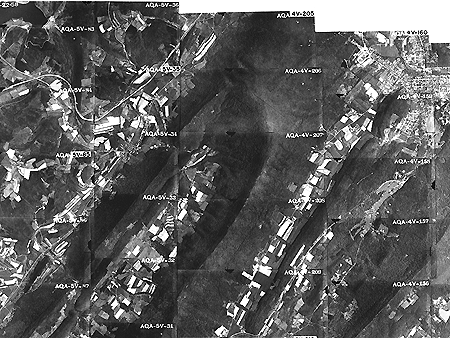
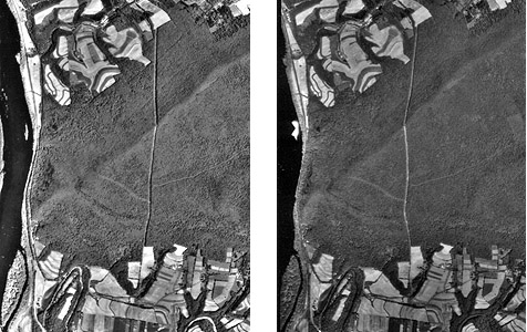
Aerial photography missions involve capturing sequences of overlapping images along many parallel flight paths. In the portion of the air photo mosaic shown below, note that the photographs overlap one another end to end and side to side. This overlap is necessary for stereoscopic viewing, which is the key to rectifying photographs of variable terrain. It takes about 10 overlapping aerial photographs taken along two adjacent north-south flightpaths to provide stereo coverage for a 7.5-minute quadrangle.

Figure 6.11.2 Portion of a mosaic of overlapping vertical aerial photographs.

Credit: United States Department of Agriculture, Commodity Stabilization Service, n.d.

This textbook is used as a resource in Penn State's Online Geospatial Education online degree and certificate programs. If this topic is interesting to you and you want to learn more about online GIS and GEOINT education at Penn State, check out our Geospatial Education Program Office.

To understand why topographic maps can't be traced directly off of most vertical aerial photographs, you first need to appreciate the difference between perspective and planimetry. In a perspective view, all light rays reflected from the Earth's surface pass through a single point at the center of the camera lens. A planimetric (plan) view, by contrast, looks as though every position on the ground is being viewed from directly above. Scale varies in perspective views. In plan views, scale is everywhere consistent (if we overlook variations in small-scale maps due to map projections). Topographic maps are said to be planimetrically correct. So are orthoimages. Vertical aerial photographs are not, unless they happen to be taken over flat terrain.

As discussed above, the scale of an aerial photograph is partly a function of flying height. Thus, variations in elevation cause variations in scale on aerial photographs. Specifically, the higher the elevation of an object, the farther the object will be displaced from its actual position away from the principal point of the photograph (the point on the ground surface that is directly below the camera lens). Conversely, the lower the elevation of an object, the more it will be displaced toward the principal point. This effect, called relief displacement, is illustrated below in Figure 6.12.1. Note that the effect increases with distance from the principal point.

Figure 6.12.1 Relief displacement is scale variation on aerial photographs caused by variations in terrain elevation.

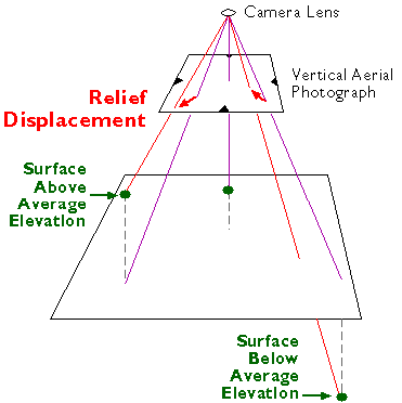
At the top of the diagram above, light rays reflected from the surface converge upon a single point at the center of the camera lens. The smaller trapezoid below the lens represents a sheet of photographic film. (The film actually is located behind the lens, but since the geometry of the incident light is symmetrical, we can minimize the height of the diagram by showing a mirror image of the film below the lens.) Notice the four triangular fiducial marks along the edges of the film. The marks point to the principal point of the photograph, which corresponds with the location on the ground directly below the camera lens at the moment of exposure. Scale distortion is zero at the principal point. Other features shown in the photo may be displaced toward or away from the principal point, depending on the elevation of the terrain surface. The larger trapezoid represents the average elevation of the terrain surface within a scene. On the left side of the diagram, a point on the land surface at a higher than average elevation is displaced outwards, away from the principal point and its actual location. On the right side, another location at less than average elevation is displaced towards the principal point. As terrain elevation increases, flying height decreases and photo scale increases. As terrain elevation decreases, flying height increases and photo scale decreases.

Compare the map and photograph below in Figure 6.12.2. Both show the same gas pipeline, which passes through hilly terrain. Note the deformation of the pipeline route in the photo relative to the shape of the route on the topographic map. The deformation in the photo is caused by relief displacement. The photo would not serve well on its own as a source for topographic mapping.

Figure 6.12.2 The pipeline clearing appears crooked in the photograph because of relief displacement.

Still confused? Think of it this way: where the terrain elevation is high, the ground is closer to the aerial camera, and the photo scale is a little larger than where the terrain elevation is lower. Although the altitude of the camera is constant, the effect of the undulating terrain is to zoom in and out. The effect of continuously-varying scale is to distort the geometry of the aerial photo. This effect is called relief displacement.

Distorted perspective views can be transformed into plan views through a process called rectification. In Summer 2001, student Joel Hamilton recounted one very awkward way to rectify aerial photographs:

"Back in the mid 80's I saw a very large map being created from a multitude of aerial photos being fitted together. A problem that arose was that roads did not connect from one photo to the next at the outer edges of the map. No computers were used to create this map. So using a little water to wet the photos on the outside of the map, the photos were stretched to correct for the distortions. Starting from the center of the map the mosaic map was created. A very messy process."

Nowadays, digital aerial photographs can be rectified in an analogous (but much less messy) way, using specialized photogrammetric software that shifts image pixels toward or away from the principal point of each photo in proportion to two variables: the elevation of the point of the Earth's surface at the location that corresponds to each pixel, and each pixel's distance from the principal point of the photo.

Another even simpler way to rectify perspective images is to view pairs of images stereoscopically.

If you have normal or corrected vision in both eyes, your view of the world is stereoscopic. Viewing your environment simultaneously from two slightly different perspectives enables you to estimate very accurately which objects in your visual field are nearer, and which are farther away. You know this ability as depth perception.

When you fix your gaze upon an object, the intersection of your two optical axes at the object form what is called a parallactic angle. On average, people can detect changes as small as 3 seconds in the parallactic angle, an angular resolution that compares well to transits and theodolites. The keenness of human depth perception is what makes photogrammetric measurements possible.

Your perception of a three-dimensional environment is produced from two separate two-dimensional images. The images produced by your eyes are analogous to two aerial images taken one after another along a flight path. Objects that appear in the area of overlap between two aerial images are seen from two different perspectives. A pair of overlapping vertical aerial images is called a stereopair. When a stereopair is viewed such that each eye sees only one image, it is possible to envision a three-dimensional image of the area of overlap.

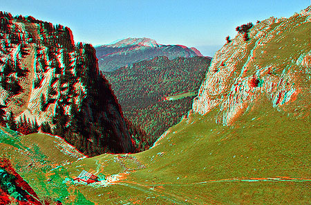
On the following page, you'll find a couple of examples of how stereoscopy is used to create planimetrically-correct views of the Earth's surface. If you have anaglyph stereo (red/blue) glasses, you'll be able to see stereo yourself. First, let's practice viewing anaglyph stereo images.

Try This!

One way to see in stereo is with an instrument called a stereoscope (see examples on the Interpreting Imagery page at James Madison University's Spatial Information Clearinghouse). Another way that works on computer screens and doesn't require expensive equipment is called anaglyph stereo (anaglyph comes from a Greek word that means, "to carve in relief"). The anaglyph method involves special glasses in which the left and right eyes are covered by blue and red filters. 

The anaglyph image shown below consists of a superimposed stereopair in which the left image is shown in red and the right image is shown in green and blue. The filters in the glasses ensure each eye sees only one image. Can you make out the three-dimensional image of the U-shaped valley formed by glaciers in the French Alps?

Figure 6.13.1 Anaglyph stereopair by Pierre Gidon showing a scene in the French Alps. Requires red/blue glasses.

Credit: The image is used by permission of the author.

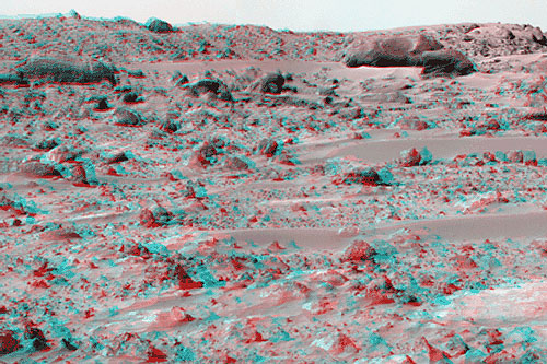
How about this one: a panorama of the surface of Mars imaged during the Pathfinder mission, July 1997?

Figure 6.13.2

Credit: NASA, 1997. Image processing and mosaic by Tim Parker.

To find other stereo images on the World Wide Web, search on "anaglyph."

This textbook is used as a resource in Penn State's Online Geospatial Education online degree and certificate programs. If this topic is interesting to you and you want to learn more about online GIS and GEOINT education at Penn State, check out our Geospatial Education Program Office.

Aerial images need to be transformed from perspective views into plan views before they can be used to trace the features that appear on topographic maps, or to digitize vector features in digital data sets. One way to accomplish the transformation is through stereoscopic viewing.

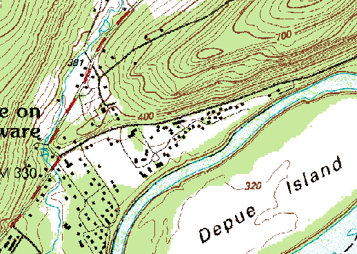
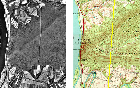
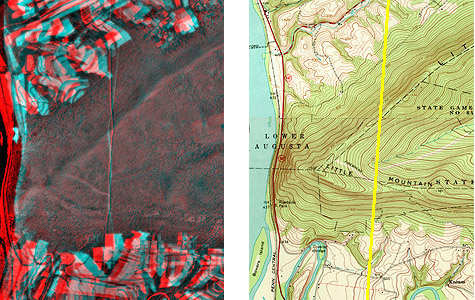
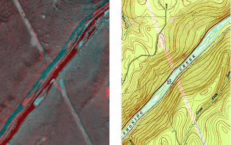
Below in Figure 6.14.1 are portions of a vertical aerial photograph and a topographic map that show the same area, a synclinal ridge called "Little Mountain" on the Susquehanna River in central Pennsylvania. A linear clearing, cut for a power line, appears on both (highlighted in yellow on the map). The clearing appears crooked on the photograph due to relief displacement. Yet we know that an aerial image like this one was used to compile the topographic map. The air photo had to have been rectified to be used as a source for topographic mapping.

Figure 6.14.1 The deformation of the powerline clearing shown in the air photo is caused by relief displacement.

Credit: USGS. "Harrisburg East Quadrangle, Pennsylvania"

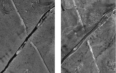
Below in Figure 6.14.2 are portions of two aerial photographs showing Little Mountain. The two photos were taken from successive flight paths. The two perspectives can be used to create a stereopair.

Figure 6.14.2 A stereopair: two air photos of the same area taken from different points of view.

Credit: USGS. "Harrisburg East Quadrangle, Pennsylvania"

Next, the stereopair is superimposed in an anaglyph image. Using your red/blue glasses, you should be able to see a three-dimensional image of Little Mountain in which the power line appears straight, as it would if you were able to see it in person. Notice that the height of Little Mountain is exaggerated due to the fact that the distance between the principal points of the two photos is not exactly proportional to the distance between your eyes.

Figure 6.14.3 An anaglyph (red/blue) stereo image that fuses the stereopair shown in the above figure. When viewed with a red filter over the left eye and a cyan (blue) filter over the right eye, a sterescopic image is formed. Notice that the powerline clearing, which appears crooked in both air photos, appears straight in the stereoscopic image.

Credit: USGS. "Harrisburg East Quadrangle, Pennsylvania"

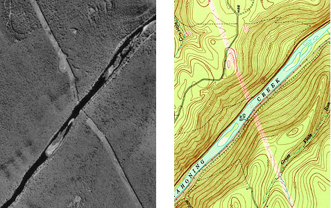
Let's try that again. We need to make sure that you can visualize how stereoscopic viewing transforms overlapping aerial photographs from perspective views into planimetric views. The aerial photograph and topographic map portions below show the same features, a power line clearing crossing the Sinnemahoning Creek in Central Pennsylvania. The power line appears to bend as it descends to the creek because of relief displacement.

Figure 6.14.4 The deformation of the powerline clearing shown in the air photo is caused by relief displacement.

Credit: USGS. "Keating Quadrangle, Pennsylvania"

Two aerial photographs of the same area taken from different perspectives constitute a stereo pair.

Figure 6.14.5 A stereopair, two air photos of the same area taken from different points of view.

Credit: USGS. "Keating Quadrangle, Pennsylvania"

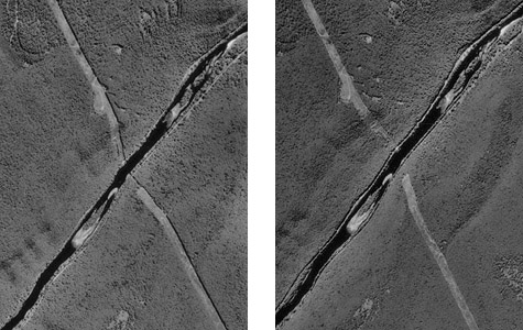
By viewing the two photographs stereoscopically, we can transform them from two-dimensional perspective views to a single three-dimensional view in which the geometric distortions caused by relief displacement have been removed.

Figure 6.14.6 Deformation caused by relief displacement is rectified when the air photos are viewed in stereo.

Credit: USGS. "Keating Quadrangle, Pennsylvania"

Photogrammetrists use instruments called stereoplotters to trace, or compile, the data shown on topographic maps from stereoscopic images like the ones you've seen here. The operator pictured below is viewing a stereoscopic model similar to the one you see when you view the anaglyph stereo images with red/blue glasses. A stereopair is superimposed on the right-hand screen of the operator's workstation. The left-hand screen shows dialog boxes and command windows through which she controls the stereoplotter software. Instead of red/blue glasses, the operator is wearing glasses with polarized lens filters that allow her to visualize a three-dimensional image of the terrain. She handles a 3-D mouse that allows her to place a cursor on the terrain image within inches of its actual horizontal and vertical position.

Figure 6.14.7 Merri MacKay (graduate of the Penn State Certificate Program in GIS, and employee of BAE Systems ADR), uses an analytic stereoplotter to digitize vertical and horizontal positions from a stereoscopic model. This photo is from circa 1998. When she encountered her picture as a student in 2004, Merri wrote "I've got short hair and four grandkids now..."

Used with permission of Ms. MacKay and ADR, Inc.

An orthoimage (or orthophoto) is a single aerial image in which distortions caused by relief displacement have been removed. The scale of an orthoimage is uniform. Like a planimetrically correct map, orthoimages depict scenes as though every point were viewed simultaneously from directly above. In other words, as if every optical axis were orthogonal to the ground surface. Notice how the power line clearing has been straightened in the orthophoto on the right, below in Figure 6.15.1.

Figure 6.15.1 Comparison of a vertical aerial photograph (left) and an orthophoto.

Relief displacement is caused by differences in elevation. If the elevation of the terrain surface is known throughout a scene, the geometric distortion it causes can be rectified. Since photogrammetry can be used to measure vertical as well as horizontal positions, it can be used to create a collection of vertical positions called a terrain model. Automated procedures for transforming vertical aerial photos into orthophotos require digital terrain models.

Since the early 1990s, orthophotos have been commonly used as sources for editing and revising of digital vector data.

Through the remainder of this chapter and the next, we'll investigate the particular data products that comprise the framework themes of the U.S. National Spatial Data Infrastructure (NSDI). The format I'll use to discuss these data products reflects the Federal Geographic Data Committee's Metadata standard (FGDC, 1998c). Metadata is data about data. It is used to document the content, quality, format, ownership, and lineage of individual data sets. As the FGDC likes to point out, the most familiar example of metadata is the "Nutrition Facts" panel printed on food and drink labels in the United States. Metadata also provides the keywords needed to search for available data in specialized clearinghouses and in the World Wide Web.

Some of the key headings included in the FGDC metadata standard include:

1. Identification Information: Who created the data, a brief description of its content, form, and purpose; its status, spatial extent, and use restrictions;
2. Data Quality Information: Accuracy and completeness of attributes, horizontal and vertical positions, sources, and procedures used to create the data;
3. Spatial Reference Information: Projection and/or coordinate system; datum and ellipsoid;
4. Entity and Attribute Information: Feature and attribute categories used; and
5. Distribution Information: Availability, and how to acquire the data.

FGDC's Content Standard for Digital Geospatial Metadata is published here. Geospatial professionals understand the value of metadata and know how to find it and how to interpret it.

Identification

Digital Orthophoto Quads (DOQs) are raster images of rectified aerial photographs. They are widely used as sources for editing and revising vector topographic data. For example, the vector roads data maintained by businesses like NAVTEQ and Tele Atlas, as well as local and state government agencies, can be plotted over DOQs, then edited to reflect changes shown in the orthoimage.

Most DOQs are produced by electronically scanning, then rectifying, black-and-white vertical aerial photographs. DOQ may also be produced from natural-color or near-infrared false-color photos, however, and from digital imagery. The variations in photo scale caused by relief displacement in the original images are removed by warping the image to compensate for the terrain elevations within the scene. Like USGS topographic maps, scale is uniform across each DOQ.

Most DOQs cover 3.75' of longitude by 3.75' of latitude. A set of four DOQs corresponds to each 7.5' quadrangle. (For this reason, DOQs are sometimes called DOQQs--Digital Orthophoto Quarter Quadrangles.) For its National Map, USGS has edge-matched DOQs into seamless data layers, by year of acquisition.

Figure 6.17.1 Portion of a USGS Digital Orthophoto Quad (DOQ) for Bushkill, PA.

Data Quality

Like other USGS data products, DOQs conform to National Map Accuracy Standards. Since the scale of the series is 1:12,000, the standards warrant that 90 percent of well-defined points appear within 33.3 feet (10.1 meters) of their actual positions. One of the main sources of error is the rectification process, during which the image is warped such that each of a minimum of 3 control points matches its known location.

Spatial Reference Information

All DOQs are cast on the Universal Transverse Mercator projection used in the local UTM zone. Horizontal positions are specified relative to the North American Datum of 1983, which is based on the GRS 80 ellipsoid.

Entities and Attributes

The fundamental geometric element of a DOQ is the picture element (pixel). Each pixel in a DOQ corresponds to one square meter on the ground. Pixels in black-and-white DOQs are associated with a single attribute: a number from 0 to 255, where 0 stands for black, 255 stands for white, and the numbers in between represent levels of gray.

DOQs exceed the scanned topographic maps shown in Digital Raster Graphics (DRGs) in both pixel resolution and attribute resolution. DOQs are therefore much larger files than DRGs. Even though an individual DOQ file covers only one-quarter of the area of a topographic quadrangle (3.75 minutes square), it requires up to 55 Mb of digital storage. Because they cover only 25 percent of the area of topographic quadrangles, DOQs are also known as Digital Orthophoto Quarter Quadrangles (DOQQs).

Distribution

USGS DOQ files are in the public domain, and can be used for any purpose without restriction. They are available for free download from the USGS, or from various state and regional data clearinghouses as well as from the geoCOMMUNITY site. Digital orthoimagery data at 1-foot and 1-meter spatial resolution, collected from multiple sources, are available for user-specified areas, and even higher resolution imagery (HRO) data sets for certain areas are available from the National Map Viewer site.

To investigate DOQ data in greater depth, including links to a complete sample metadata document, visit Birthplace of the DOQ.  FGDC's Content Standard for Digital Orthoimagery is published here.

This textbook is used as a resource in Penn State's Online Geospatial Education online degree and certificate programs. If this topic is interesting to you and you want to learn more about online GIS and GEOINT education at Penn State, check out our Geospatial Education Program Office.

Many local, state, and federal government agencies produce and rely upon geographic data to support their day-to-day operations. The National Spatial Data Infrastructure (NSDI) is meant to foster cooperation among agencies to reduce costs and increase the quality and availability of public data in the U.S. The key components of NSDI include standards, metadata, data, a clearinghouse for data dissemination, and partnerships. The seven framework data themes have been described as "the data backbone of the NSDI" (FGDC, 1997, p. v). This chapter and the next review the origins, characteristics and status of the framework themes. In comparison with some other developed countries, framework data are fragmentary in the U.S., largely because mapping activities at various levels of government remain inadequately coordinated.

Chapter 6 considers two of the seven framework themes: geodetic control and orthoimagery. It discusses the impact of high-accuracy satellite positioning on accuracy standards for the National Spatial Reference System--the U.S.' horizontal and vertical control networks. The chapter stresses the fact that much framework data is derived, directly or indirectly, from aerial imagery. Geospatial professionals understand how photogrammetrists compile planimetrically-correct vector data by stereoscopic analysis of aerial imagery. They also understand how orthoimages are produced and used to help keep vector data current, among other uses.

The most ambitious attempt to implement a nationwide collection of framework data is the USGS' National Map. Composed of some of the digital data products described in this chapter and those that follow, the proposed National Map is to include high resolution (1 m) digital orthoimagery, variable resolution (10-30 m) digital elevation data, vector transportation, hydrography, and boundaries, medium resolution (30 m) land characterization data derived from satellite imagery, and geographic names. These data are to be seamless (unlike the more than 50,000 sheets that comprise the 7.5-minute topographic quadrangle series) and continuously updated. Meanwhile, in 2005, USGS announced that two of its three National Mapping Centers (in Reston, Virginia and Rolla, Missouri) would be closed, and over 300 jobs eliminated. Although funding for the Rolla center was subsequently restored by Congress, it remains to be seen whether USGS will be sufficiently resourced to fulfill its quest for a National Map.

This textbook is used as a resource in Penn State's Online Geospatial Education online degree and certificate programs. If this topic is interesting to you and you want to learn more about online GIS and GEOINT education at Penn State, check out our Geospatial Education Program Office.