The previous section highlighted the one-meter panchromatic data produced by the IKONOS satellite sensor. Pan data is not all that IKONOS produces, however. It is a multispectral sensor that records reflectances within four other (narrower) bands, including the blue, green, and red wavelengths of the visible spectrum, and the near-infrared band. The range(s) of wavelengths that a sensor is able to detect is called its spectral sensitivity.
| Spectral Sensitivity | Spatial Resolution |
|---|---|
| 0.45 - 0.90 µm (panchromatic) | 1m |
| 0.45 - 0.52 µm (visible blue) | 4m |
| 0.51 - 0.60 µm (visible green) | 4m |
| 0.63 - 0.70 µm (visible red) | 4m |
| 0.76 - 0.85 µm (near IR) | 4m |
Spectral sensitivities and spatial resolution of the IKONOS I sensor. Wavelengths are expressed in micrometers (millionths of a meter). Spatial resolution is expressed in meters.
This section profiles two families of multispectral sensors that play important roles in land use and land cover characterization: AVHRR and Landsat.
AVHRR
AVHRR stands for "Advanced Very High Resolution Radiometer." AVHRR sensors have been onboard sixteen satellites maintained by the National Oceanic and Atmospheric Administration (NOAA) since 1979 (TIROS-N, NOAA-6 through NOAA-15). The data the sensors produce are widely used for large-area studies of vegetation, soil moisture, snow cover, fire susceptibility, and floods, among other things.
AVHRR sensors measure electromagnetic energy within five spectral bands, including visible red, near infrared, and three thermal infrared. The visible red and near-infrared bands are particularly useful for large-area vegetation monitoring. The Normalized Difference Vegetation Index (NDVI), a widely used measure of photosynthetic activity that is calculated from reflectance values in these two bands, is discussed later.
| Spectral Sensitivity | Spatial Resolution |
|---|---|
| 0.58 - 0.68 µm (visible red) | 1-4 km* |
| 0.725 - 1.10 µm (near IR) | 1-4 km* |
| 3.55 - 3.93 µm (thermal IR) | 1-4 km* |
| 10.3 - 11.3 µm (thermal IR) | 1-4 km* |
| 11.5 - 12.5 µm (thermal IR) | 1-4 km* |
Spectral sensitivities and spatial resolution of the AVHRR sensor. Wavelengths are expressed in micrometers (millionths of a meter). Spatial resolution is expressed in kilometers (thousands of meters). *Spatial resolution of AVHRR data varies from 1 km to 16 km. Processed data consist of uniform 1 km or 4 km grids.
The NOAA satellites that carry AVHRR sensors trace sun-synchronous polar orbits at altitudes of about 833 km. Traveling at ground velocities of over 6.5 kilometers per second, the satellites orbit the Earth 14 times daily (every 102 minutes), crossing over the same locations along the equator at the same times every day. As it orbits, the AVHRR sensor sweeps a scan head along a 110°-wide arc beneath the satellite, taking many measurements every second. (The back and forth sweeping motion of the scan head is said to resemble a whisk-broom.) The arc corresponds to a ground swath of about 2400 km. Because the scan head traverses so wide an arc, its instantaneous field of view (IFOV: the ground area covered by a single pixel) varies greatly. Directly beneath the satellite, the IFOV is about 1 km square. Near the edge of the swath, however, the IFOV expands to over 16 square kilometers. To achieve uniform resolution, the distorted IFOVs near the edges of the swath must be resampled to a 1 km grid (Resampling is discussed later in this chapter). The AVHRR sensor is capable of producing daily global coverage in the visible band, and twice daily coverage in the thermal IR band.
For more information, visit the USGS' AVHRR home page.
Landsat MSS
Television images of the Earth taken from early weather satellites (such as TIROS-1, launched in 1960), and photographs taken by astronauts during the U.S. manned space programs in the 1960s, made scientists wonder about how such images could be used for environmental resource management. In the mid 1960s, U.S. National Aeronautics and Space Administration (NASA) and the Department of Interior began work on a plan to launch a series of satellite-based orbiting sensors. The Earth Resource Technology Satellite program launched its first satellite, ERTS-1, in 1972. When the second satellite was launched in 1975, NASA renamed the program Landsat. Since then, there have been six successful Landsat launches (Landsat 6 failed shortly after takeoff in 1993; Landsat 7 successfully launched in 1999).
Two sensing systems were on board Landsat 1 (formerly ERTS-1): a Return Beam Videcon (RBV) and a Multispectral Scanner (MSS). The RBV system is analogous to today's digital cameras. It sensed radiation in the visible band for an entire 185 km square scene at once, producing images comparable to color photographs. The RBV sensor was discontinued after Landsat 3, due to erratic performance and a general lack of interest in the data it produced.
The MSS sensor, however, enjoyed much more success. From 1972 through 1992, it was used to produce an archive of over 630,000 scenes. MSS measures radiation within four narrow bands: one that spans visible green wavelengths, another that spans visible red wavelengths, and two more spanning slightly longer, near-infrared wavelengths.
| Spectral Sensitivity | Spatial Resolution |
|---|---|
| 0.5 - 0.6 µm (visible green) | 79 / 82 m* |
| 0.6 - 0.7 µm (visible red) | 79 / 82 m* |
| 0.7 - 0.8 µm (near IR) | 79 / 82 m* |
| 0.8 - 1.1 µm (near IR) | 79 / 82 m* |
Spectral sensitivities and spatial resolution of the Landsat MSS sensor. Wavelengths are expressed in micrometers (millionths of a meter). Spatial resolution is expressed in meters. *MSS sensors aboard Landsats 4 and 5 had nominal resolution of 82 m, which includes 15 meters of overlap with previous scene.
Landsats 1 through 3 traced near-polar orbits at altitudes of about 920 km, orbiting the Earth 14 times per day (every 103 minutes). Landsats 4 and 5 orbit at 705 km altitude. The MSS sensor sweeps an array of six energy detectors through an arc of less than 12°, producing six rows of data simultaneously across a 185 km ground swath. Landsat satellites orbit the Earth at similar altitudes and velocities as the satellites that carry AVHRR, but because the MSS scan swath is so much narrower than AVHRR, it takes much longer (18 days for Landsat 1-3, 16 days for Landsats 4 and 5) to scan the entire Earth's surface.
The sequence of three images shown above cover the same portion of the state of Rondonia, Brazil. Reflectances in the near-infrared band are coded red in these images; reflectances measured in the visible green and red bands are coded blue and green. Since vegetation absorbs visible light, but reflects infrared energy, the blue-green areas indicate cleared land. Land use change detection is one of the most valuable uses of multispectral imaging.
For more information, visit USGS' Landsat home page.
Landsat TM and ETM+
As NASA prepared to launch Landsat 4 in 1982, it replaced the unsuccessful RBV sensor with a new sensing system called Thematic Mapper (TM). TM was a new and improved version of MSS that featured higher spatial resolution (30 meters in most channels) and expanded spectral sensitivity (seven bands, including visible blue, visible green, visible red, near-infrared, two mid-infrared, and thermal infrared wavelengths). An Enhanced Thematic Mapper Plus (ETM+) sensor, which includes an eighth (panchromatic) band with a spatial resolution of 15 meters, was onboard Landsat 7 when it successfully launched in 1999.
| Spectral Sensitivity | Spatial Resolution |
|---|---|
| 0.522 -0.90 µm (panchromatic)* | 15 m* |
| 0.45 - 0.52 µm (visible blue) | 30 m |
| 0.52 - 0.60 µm (visible green) | 30 m |
| 0.63 - 0.69 µm (visible red) | 30 m |
| 0.76 - 0.90 µm (near IR) | 30 m |
| 1.55 - 1.75 µm (mid IR) | 30 m |
| 10.40 - 12.50 µm (thermal IR) | 120 m (Landsat 4-5) 60 m (Landsat 7) |
| 2.08 - 2.35 µm (mid IR) | 30 m |
Spectral sensitivities and spatial resolution of the Landsat TM and ETM sensors. Wavelengths are expressed in micrometers (millionths of a meter). Spatial resolution is expressed in meters. Note the lower spatial resolution in thermal IR band, which allows for increased radiometric resolution. *ETM+/Landsat 7 only.
The spectral sensitivities of the TM and ETM+ sensors are attuned to both the spectral response characteristics of the phenomena that the sensors are designed to monitor, as well as to the windows within which electromagnetic energy are able to penetrate the atmosphere. The following table outlines some of the phenomena that are revealed by each of the wavelengths bands, phenomena that are much less evident in panchromatic image data alone.
| Band | Phenomena Revealed |
|---|---|
| 0.45 - 0.52 µm (visible blue) | Shorelines and water depths (these wavelengths penetrate water) |
| 0.52 - 0.60 µm (visible green) | Plant types and vigor (peak vegetation reflects these wavelengths strongly) |
| 0.63 - 0.69 µm (visible red) | Photosynthetic activity (plants absorb these wavelengths during photosynthesis) |
| 0.76 - 0.90 µm (near IR) | Plant vigor (healthy plant tissue reflects these wavelengths strongly) |
| 1.55 - 1.75 µm (mid IR) | Plant water stress, soil moisture, rock types, cloud cover vs. snow |
| 10.40 - 12.50 µm (themal IR) | Relative amounts of heat, soil moisture |
| 2.08 - 2.35 µm (mid IR) | Plant water stress, mineral and rock types |
Until 1984, Landsat data were distributed by the U.S. federal government (originally by the USGS's EROS Data Center, later by NOAA). Data produced by Landsat missions 1 through 4 are still available for sale from EROS. With the Land Remote Sensing Commercialization Act of 1984, however, the U.S. Congress privatized the Landsat program, transferring responsibility for construction and launch of Landsat 5, and for distribution of the data it produced, to a firm called EOSAT.
Dissatisfied with the prohibitive costs of unsubsidized data (as much as $4,400 for a single 185 km by 170 km scene), users prompted Congress to pass the Land Remote Sensing Policy Act of 1992. The new legislation returned responsibility for the Landsat program to the U.S. government. Data produced by Landsat 7 is distributed by USGS at a cost to users of $600 per scene (about 2 cents per square kilometer). Scenes that include data gaps caused by a "scan line corrector" failure are sold for $250; $275 for scenes in which gaps are filled with earlier data.
Try This!
You may choose to visit the USGS' EarthNow! Landsat Image Viewer, which allows you to view live acquisition of Landsat 5 and Landsat 7 images. This site has a link to the USGS Global Visualization Viewer where you can search for images based on percent cloud cover.

Landsat OLI and TIRS
The NASA mission known as the Landsat Data Continuity Mission (LDCM) launched the Landsat 8 satellite in February of 2013. The satellite payload, or observatory as it is referred to, includes two sensors, the Operational Land Imager (OLI) and the Thermal Infrared Sensor (TIRS).
The spatial resolution of the Landsat 8 data is comparable to that of the Landsat 7 data. Compare the Spatial Resolution column of Table 8.6 to Table 8.4.
When it comes to spectral resolution, six of the Landsat 8 bands have wavelength ranges that are comparable to bands of Landsat 7, but they have been refined somewhat. For example, the NIR band has been fine-tuned in order to decrease the effects of atmospheric absorption. Compare Table 8.6 to Table 8.5, and see Figure 8.12.4 below.
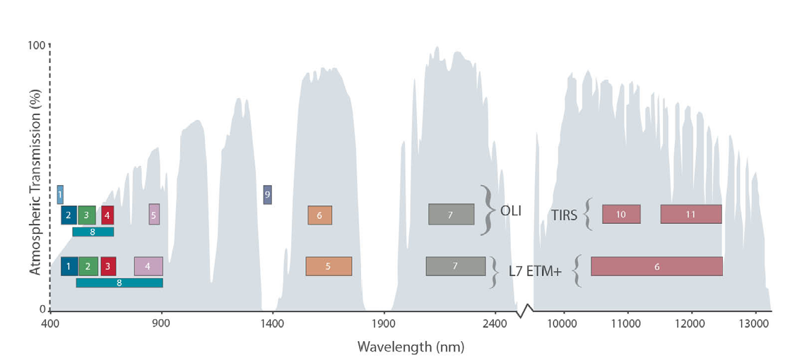
The OLI collects data at 30-meter resolution in eight shortwave (SW) spectral bands, and in one panchromatic band at a 15-meter resolution. The two new spectral bands are a deep-blue band that increases the coverage of coastal areas, and a band for the detection of cirrus cloud coverage. Being able to measure the cirrus cloud coverage can alert the researcher to the need for an image collected on cloud-free day, or it can enable the negative effects of these high-altitude clouds to be corrected for.
The TIRS collects data from two long wave thermal bands at a resolution of 100 meters. Compared to the single long wave thermal band collected by Landsat 7 these two bands are better suited for thermal imaging mapping and to support such new applications as modeling evapotranspiration over irrigated fields.
The Landsat 8 instruments provide higher radiometric resolution data than Landsat 7. Landsat 8 collects data with a bit depth of 12 bits per pixel, which provides the ability to distinguish up to 4096 different reflectance values. This capability will help in the study of the finer reflectance differences characteristic of snow- and ice-covered regions.
Landsat 7 is still collecting data. Landsat 8 orbits at the same altitude as Landsat 7. Both satellites complete an orbit in 99 minutes, and complete close to 14 orbits per day. This results in every point on Earth being crossed every 16 days. But, because the orbits of the two satellites are offset, it results in repeat coverage every 8 days. Approximately 1000 images per day are collected by Landsat 7 and Landsat 8 combined. That is almost double the images collected when Landsat 5 and Landsat 7 were operating concurrently
| Spectral Bands | Spatial Resolution | Phenomena Revealed/Use |
|---|---|---|
| 0.43 - 0.45 μm (Band 1 - visible deep-blue) |
30 m | Coastal/aerosol; increased coastal zone observations |
| 0.45 - 0.51 μm (Band 2 - visible blue) |
30 m | Bathymetric mapping; distinguishes soil from vegetation; deciduous from coniferous vegetation |
| 0.53 - 0.59 μm (Band 3 - visible green) |
30 m | Emphasizes peak vegetation, which is useful for assessing plant vigor |
| 0.64 - 0.67 μm (Band 4 - visible red) |
30 m | Emphasizes vegetation on slopes |
| 0.85 - 0.88 μm (Band 5 - near IR) |
30 m | Emphasizes vegetation boundary between land and water, and landforms |
| 1.57 - 1.65 μm (Band 6 - SWIR 1) |
30 m | Used in detecting plant drought stress and delineating burnt areas and fire-affected vegetation, and is also sensitive to the thermal radiation emitted by intense fires; can be used to detect active fires, especially during nighttime when the background interference from SWIR in reflected sunlight is absent |
| 2.11 – 2.29 μm (Band 7 - SWIR-1) |
30 m | Used in detecting drought stress, burnt and fire-affected areas, and can be used to detect active fires, especially at nighttime |
| 0.50 – 0.68 μm (Band 8 - panchromatic) |
15 m | Useful in ‘sharpening’ multispectral images |
| 1.36 – 1.38 μm (Band 9 - cirrus) |
30 m | Useful in detecting cirrus clouds |
| 10.60 - 11.19 μm (Band 10 - Thermal IR 1) |
100 m | Useful for mapping thermal differences in water currents, monitoring fires and other night studies, and estimating soil moisture |
| 11.50 - 12.51 μm (Band 11 - Thermal IR 2) |
100 m | Same as band 10 |
Spectral sensitivities, spatial resolution of Landsat 8 sensors, and what the data can be used for. The band designation numbers of the 11 bands are included. Wavelengths are expressed in micrometers (millionths of a meter). Spatial resolution is expressed in meters.