Lessons
Lesson 1: Advanced Python and Multiprocessing
Lesson 1 is one week in length and serves as a refresher and preparation for the rest of the course. You may already know many of the topics covered in the modules and want to skip over them, but it may be worth skimming though the topic. The assignment will walk you through implementing multiprocessing to clip a set of feature classes in parallel. Don’t stress out too much about this, much of the necessary coding and process will be provided to you.
The Integrated Development Environment (IDE) we are going to start with in this class is called PyScripter, but feel free to use another IDE that you are comfortable with. We will start the lesson with discussing the debugger. Learning how to use this tool will save you time and save you from many headaches. I encourage you to spend some time learning how to use it since it is cleaner, faster, and provides more infomration than print statements. It will also help you identify errors and execution misteps throughout your code.
Next, we will look at Python types and structures, logic constructs, methods/functions, and finish the lesson with multiprocessing.
Overview and Checklist
The lesson contains a lot of material, but it reads quickly. If there is a portion that is not clear or if you have questions, please feel free to use the canvas discussion boards and post your questions to the class. If you can answer a question, please feel free to answer it.
Pace yourself and leave plenty of time for working on the assignment. If you have completed the assignment and want to try your hand at implementing a different means of multi-processing or try it on another process that may benefit your work, I encourage you try it and submit the code. There are many solutions and implementations so feel free to explore them and find one that works for your process.
Learning Outcomes
- Utilize the debugger and interpret its output.
- Identify and properly use Python types and functions.
- Execute a task using multiprocessing.
Lesson Roadmap
| Step | Activity | Access/Directions |
|---|---|---|
| 1 | Engage with Lesson 1 Content | Begin with Debugging. |
| 2 | Programming Assignment and Reflection | Submit your code for the programming assignment and 400 words write-up with reflections |
| 3 | Quiz 1 | Complete the Lesson 1 Quiz |
| 4 | Questions/Comments | Remember to visit Canvas to post/answer any questions or comments pertaining to Lesson 3 |
Downloads
The following is a list of datasets that you will be prompted to download through the course of the lesson. They are divided into two sections: Datasets that you will need for the assignments and Datasets used for the content and examples in the lesson.
Required:
Suggested:
- USA.gdb.zip [2]
- In the Multiprocessing with raster data section you will also use some DEM raster data that you can download here [3] if you want to follow along with the content. You can also wait with obtaining that data until you reach that section in the lesson material.
Assignments
We are going to use the arcpy vector data processing code from Multiprocessing with vector data (download Lesson1_Assignment_initial_code.zip [1]) as the basis for our Lesson 1 programming project. The code is already in multiprocessing mode, so you will not have to write multiprocessing code on your own from scratch but you still will need a good understanding of how the script works. If you are unclear about anything the script does, please ask on the course forums. This part of the assignment will be for getting back into the rhythm of writing arcpy based Python code and practice creating a multiprocessing script. Your task is to extend our vector data clipping script by doing the following:
Expand the code so that it can handle multiple input feature classes to be clipped (still using a single polygon clipping feature class). The input variable data_to_be_clipped should now take a list of feature class names rather than a single name. The worker function should, as before, perform the operation of clipping a single input file (not all of them!) to one of the features from the clipper feature class. The main change you will have to make will be in the main code where the jobs are created. The names of the output files produced should have the format
clip_<oid>_<name of the input feature class>.shp
For instance clip_0_Roads.shp for clipping the Roads feature class from USA.gdb to the state featureclass with oid 0. You can change the OID to the state name if you want to expand the code.
Submit a single .zip file to the corresponding drop box on Canvas; the zip file should contain:
- Your modified code files. Please organize the files cleanly.
- A 400-word write-up of what you have learned during this exercise.
Questions?
If you have any questions, please send a message through Canvas. We will check daily to respond. If your question is one that is relevant to the entire class, we may respond to the entire class rather than individually.
Debugging
Debugging is a very important part of writing code. The simplest method of debugging is to embed print statements in your code to either determine how far your code is running through a loop or to print out the contents of a variable. This works to some degree, but it does not tell you why your code failed where it did. A more detailed method involves using the tools or features of your IDE to create watches for checking the contents of variables and breakpoints for stepping through your code.
We will provide a generic overview of the techniques here of setting breakpoints, watches, and stepping through code. Don’t focus on the specifics of the interface as we do this. Instead, it is more important to understand the purpose of each of the different methods of debugging. The debugger will be your greatest tool for writing code and working through complex processes since it will allow to inspect your variables, data, and step through your application's or script's execution flow.
We will start off by looking at PyScripter debugging functions. There's more details of the different debugging Engines in the PyScripter Debugger [4] wiki. For this class, the standard debugger will work.
The best way to explain the aspects of debugging is to work through an example. This time, we'll look at some code that tries to calculate the factorial of an integer (the integer is hard-coded to 5 in this case). In mathematics, a factorial is the product of an integer and all positive integers below it. Thus, 5! (or "5 factorial") should be
5 * 4 * 3 * 2 * 1 = 120
The code below attempts to calculate a factorial through a loop that increments the multiplier by 1 until it reaches the original integer. This is a valid approach since 1 * 2 * 3 * 4 * 5 would also yield 120.
# This script calculates the factorial of a given
#  integer, which is the product of the integer and
#  all positive integers below it.

number = 5
multiplier = 1

while multiplier < number:
    number *= multiplier
    multiplier += 1

print (number)
Even if you can spot the error, follow along with the steps below to get a feel for the debugging process and the PyScripter Debug toolbar.
Open PyScripter and copy the above code into a new script.
- Save your script as debugger_walkthrough.py. You can optionally run the script, but you won't get a result.
- Click View > Toolbars and ensure Debug is checked. You should see a toolbar like this:
 Many IDEs have debugging toolbars like this, and the tools they contain are pretty standard: a way to run the code, a way to set breakpoints, a way to step through the code line by line, and a way to watch the value of variables while stepping through the code. We'll cover each of these in the steps below.
 - Move your cursor to the left of line 5 (number = 5) and click. If you are in the right area, you will see a red dot next to the line number, indicating the addition of a breakpoint. A breakpoint is a place where you want your code to stop running, so you can examine it line by line using the debugger. Often you'll set a breakpoint deep in the middle of your script, so you don't have to examine every single line of code. In this example, the script is very short, so we're putting the breakpoint right at the beginning. The breakpoint is represented by a circle next to the line of code, and this is common in other debuggers too.
 Note that F5 is the shortcut key for this command.
 - Press the Debug file
 button . This runs your script up to the breakpoint. In the Python Interpreter console, note that the debugfile() function is run on your script rather than the normal runfile() function. Also, instead of the normal >>> prompt, you should now see a [Dbg]>>> prompt. The cursor will be on that same line in PyScripter's Editor pane, which causes that line to be highlighted.
 - Click the Step over next function call button
 or the Step into subroutine
  button. This executes the line of your code, in this case the number = 5 line. Both buttons execute the highlighted statement, but it is important to note here that they will behave differently when the statement includes a call to a function. The Step over next function call button will execute all the code within the function, return to your script, and then pause at the script's next line. You'd use this button when you're not interested in debugging the function code, just the code of your main script. The Step into subroutine button, on the other hand, is used when you do want to step through the function code one line at a time. The two buttons will produce the same behavior for this simple script. You'll want to experiment with them later in the course when we discuss writing our own functions and modules.
 - Before going further, click the Variable window tab in PyScripter's lower pane. Here, you can track what happens to your variables as you execute the code line by line. The variables will be added automatically as they are encountered. At this point, you should see a globals {}, which contain variables from the python packages and locals {} that will contain variables created by your script. We will be looking at the locals dictionary so you can disregard the globals. Expanding the locals dictionary, you should see some are built in variables (__<name>__) and we can ignore those for now. The "number" variable should be listed, with a type of int. Expanding on the +, will expose more of the variables properties.
- Click the Step button again. You should now see the "multiplier" variable has been added in the Variable window, since you just executed the line that initializes that variable, as called out in the image.

- Click the Step button a few more times to cycle through the loop. Go slowly, and use the Variable window to understand the effect that each line has on the two variables. (Note that the keyboard shortcut for the Step button is F8, which you may find easier to use than clicking on the GUI.) Setting a watch on a variable is done by placing the cursor on the variable and then pressing Alt+W or right clicking in the Watches pane and selecting Add Watch At Cursor. This isolates the variable to the Watch window and you can watch the value change as it changes in the code execution.

-
Step through the loop until "multiplier" reaches a value of 10. It should be obvious at this point that the loop has not exited at the desired point. Our intent was for it to quit when "number" reached 120.
Can you spot the error now? The fact that the loop has failed to exit should draw your attention to the loop condition. The loop will only exit when "multiplier" is greater than or equal to "number." That is obviously never going to happen as "number" keeps getting bigger and bigger as it is multiplied each time through the loop.
In this example, the code contained a logical error. It re-used the variable for which we wanted to find the factorial (5) as a variable in the loop condition, without considering that the number would be repeatedly increased within the loop. Changing the loop condition to the following would cause the script to work:
while multiplier < 5:
Even better than hard-coding the value 5 in this line would be to initialize a variable early and set it equal to the number whose factorial we want to find. The number could then get multiplied independent of the loop condition variable.
-
Click the Stop button in the Debug toolbar to end the debugging session. We're now going to step through a corrected version of the factorial script, but you may notice that the Variable window still displays a list of the variables and their values from the point at which you stopped executing. That's not necessarily a problem, but it is good to keep in mind.
-
Open a new script, paste in the code below, and save the script as debugger_walkthrough2.py
# This script calculates the factorial of a given # integer, which is the product of the integer and # all positive integers below it. number = 5 loopStop = number multiplier = 1 while multiplier < loopStop: number *= multiplier multiplier += 1 print (number) - Step through the loop a few times as you did above. Watch the values of the "number" and "multiplier" variables, but also the new "loopStop" variable. This variable allows the loop condition to remain constant while "number" is multiplied. Indeed, you should see "loopStop" remain fixed at 5 while "number" increases to 120.
- Keep stepping until you've finished the entire script. Note that the usual >>> prompt returns to indicate you've left debugging mode.
In the above example, you used the Debug toolbar to find a logical error that had caused an endless loop in your code. Debugging tools are often your best resource for hunting down subtle errors in your code.
You can and should practice using the Debug toolbar in the script-writing assignments that you receive in this course. Spending a little time to master the few simple steps of the debugger will save you tremendous amounts of time troubleshooting.
Import and Some Syntactic Sugar
Now that we are familiar with how to step into the code and look at our variables, lets warm up a bit and briefly revisit a few Python features that you are already familiar with but for which there exist some forms or details that you may not yet know. We will start with the Python “import” command and introduce a few Python constructs that you may be new to you on the way.
It is highly recommended that you try these examples yourself, experiment with them to get a better understanding, and use the debugger to step into the process to explore and see the variables values.
Import
What happens here is that the module (either a module from the standard library, a module that is part of another package you installed, or simply another .py file in your project directory) is loaded, unless it has already been loaded before, and the name of the module becomes part of the namespace of the script that contains the import command. As a result, you can now access all variables, functions, or classes defined in the imported module, by writing
<module name>.<variable or function name>
e.g.,
arcpy.Describe(…)
You can also use the import command like this instead:
import arcpy as ap
This form introduces a new alias for the module name, typically to save some typing when the module name is rather long, and instead of writing
arcpy.Describe(…)
you would now use
ap.Describe(…)
in your code. Note that the use of ‘…’ is to indicate parameters, code between two important lines of code that would otherwise be distracting or is not necessary to show, or a continuation of list items.
Another approach of using “import” is to directly add content of a module (again either variables, functions, or classes) to the namespace of the importing Python script. This is done by using the form "from … import …" as in the following example:
from arcpy import Describe, Point , …

...

Describe(…)
The difference is that now you can use the imported names directly in our code without having to use the module name (or an alias) as a prefix as it is done in line 5 of the example code. However, be aware that if you are importing multiple modules, this can easily lead to name conflicts if, for instance, two modules contain functions with the same name. It can also make your code a little more difficult to read since
arcpy.Describe(...)
helps you or another programmer recognize that you’re using something defined in arcpy and not in another library or the main code of your script.
You can also use
from arcpy import *
to import all variable, function and class names from a module into the namespace of your script if you don’t want to list all those you actually need. However, this can increase the likelihood of a name conflict.
Keep in mind that readability matters and using the <module name>.<variable or function name> helps the reader know where the function is coming from. Modules may have similar function names and this convention helps describe which package you are using. Your IDE might flag the function as ambiguous if it finds any same named function declarations that could be from multiple modules.
Lesson content developed by Jan Wallgrun and James O’Brien
Python data types
Python contains many data types built in. These include text, numeric, sequence, mapping, sets, Boolean, binary and None. Coding at its core is largely working with data that is in one of these types and it is important to know them and how they work.
As a developer, you need to know types for operations and for parameters and this helps with debugging, performing conditionals, calculations, dictionary operations, and data transformations. For example, the string “1” does not equal the int 1. Trying to add “2” + 5 will result in a TypeError
res = "2" + 5
print (res)
Output
Traceback (most recent call last): TypeError: can only concatenate str (not "int") to str
Changing the 5 to “5” results in concatenation of the “2” and “5”:
res = "2" + "5"
print (res)
Output
25
For this course, we will be looking at more advanced structures in the mapping type. W3 provides a great overview of the data types [5] and I encourage you to review them.
Variables: local vs. global, mutable vs. immutable
When making the transition from a beginner to an intermediate or advanced Python programmer, it also gets important to understand the intricacies of variables used within functions and of passing parameters to functions in detail. First of all, we can distinguish between global and local variables within a Python script. Global variables are defined outside of any function or loop construct, or with the keyword global. They can be accessed from anywhere in the script after they are instantiated. They exist and keep their values as long as the script is loaded, which typically means as long as the Python interpreter into which they are loaded is running.
In contrast, local variables are defined inside a function or loop construct and can only be accessed in the body (scope) of that function or loop. Furthermore, when the body of the function has been executed, its local variables will be discarded and cannot be used anymore to access their current values. A local variable is either a parameter of that function, in which case it is assigned a value immediately when the function is called, or it is introduced in the function body by making an assignment to the name for the first time.
Here are a few examples to illustrate the concepts of global and local variables and how to use them in Python.
def doSomething(x):  # parameter x is a local variable of the function
    count = 1000 * x  # local variable count is introduced
    return count

y = 10  # global variable y is introduced
print(doSomething(y))
print(count)  # this will result in an error
print(x)  # this will also result in an error
This example introduces one global variable, y, and two local variables, x and count, both part of the function doSomething(…). x is a parameter of the function, while count is introduced in the body of the function in line 3. When this function is called in line 11, the local variable x is created and assigned the value that is currently stored in global variable y, so the integer number 10. Then the body of the function is executed. In line 3, an assignment is made to variable count. Since this variable hasn’t been introduced in the function body before, a new local variable will now be created and assigned the value 10000. After executing the return statement in line 5, both x and count will be discarded. Hence, the two print statements at the end of the code would lead to errors because they try to access variables that do not exist anymore.
Think of the function as a house with one-way mirrored windows. You can see out, but cannot see in. Variables, can ‘see’ to the outside, but a variable on the outside cannot see 'into' the function. This is also referred to as variable scope. The scope of the variable is where the variable is created and follows the code indents, unless it is decorated with global. Simply, inner scopes can access the outer scopes, but the outer scopes cannot reach into the inner scopes.
Now let’s change the example to the following:
def doSomething():
    count = 1000 * y    # global variable y is accessed here
    return count
y = 10
print(doSomething())
This example shows that global variable y can also be directly accessed from within the function doSomething(): When Python encounters a variable name that is neither the name of a parameter of that function nor has been introduced via an assignment previously in the body of that function, it will look for that variable among the global (outer scope) variables. However, the first version using a parameter instead is usually preferable because then the code in the function doesn’t depend on how you name and use variables outside of it. That makes it much easier to, for instance, re-use the same function in different projects.
So maybe you are wondering whether it is also possible to change the value of a global variable from within a function, not just read its value? One attempt to achieve this could be the following:
def doSomething():
    count = 1000
    y = 5
    return count * y
y = 10
print(doSomething())
print(y)  # output will still be 10 here
However, if you run the code, you will see that last line still produces the output 10, so the global variable y hasn't been changed by the assignment in line 5. That is because the rule is if the variable is not passed to the function or the variable is not marked as global within the function, it will be considered a local variable to that function. Since this is the first time an assignment to y is made in the body of the function, a new local variable with that name is created at that point that will overshadow the global variable with the same name until the end of the function has been reached. Instead, you explicitly must tell Python that a variable name should be interpreted as the name of a global variable by using the keyword ‘global’, like this:
def doSomething():
    count = 1000
    global y  # tells Python to treat y as the name of global variable
    y = 5  # as a result, global variable y is assigned a new value here
    return count * y


y = 10
print(doSomething())
print(y)  # output will now be 5 here
In line 5, we are telling Python that y in this function should refer to the global variable y. As a result, the assignment in line 7 changes the value of the global variable called y and the output of the last line will be 5. While it's good to know how these things work in Python, we again want to emphasize that accessing global variables from within functions should be avoided as much as possible. Passing values via parameters and returning values is usually preferable because it keeps different parts of the code as independent of each other as possible.
So after talking about global vs. local variables, what is the issue with mutable vs. immutable mentioned in the heading? There is an important difference in passing values to a function depending on whether the value is from a mutable or immutable data type. All values of primitive data types like numbers and boolean values in Python are immutable, meaning you cannot change any part of them. On the other hand, we have mutable data types like lists and dictionaries for which it is possible to change their parts: You can, for instance, change one of the elements in a list or what is stored under a particular key in a given dictionary without creating a completely new object.
What about strings and tuples? You may think these are mutable objects, but they are actually immutable. While you can access a single character from a string or element from a tuple, you will get an error message if you try to change it by using it on the left side of the equal sign in an assignment. Moreover, when you use a string method like replace(…) to replace all occurrences of a character by another one, the method cannot change the string object in memory for which it was called but has to construct a new string object and return that to the caller.
Why is that important to know in the context of writing functions? Because mutable and immutable data types are treated differently when provided as a parameter to functions as shown in the following two examples:
def changeIt(x):
    x = 5  # this does not change the value assigned to y because x is considered local


y = 3
changeIt(y)
print(y)  # will print out 3
As we already discussed above, the parameter x is treated as a local variable in the function body. We can think of it as being assigned a copy of the value that variable y contains when the function is called. As a result, the value of the global variable y doesn’t change and the output produced by the last line is 3. But it only works like this for immutable objects, like numbers in this case! Let’s do the same thing for a list:
def changeIt(x):
    x[0] = 5  # this will change the list y refers to

y = [3, 5, 7]
changeIt(y)
print(y)  # output will be [5, 5, 7]
The output [5, 5, 7] produced by the print statement in the last line shows that the assignment in line 3 changed the list object that is stored in global variable y. How is that possible? Well, for values of mutable data types like lists, assigning the value to function parameter x cannot be conceived as creating a copy of that value and, as a result, having the value appear twice in memory. Instead, x is set up to refer to the same list object in memory as y. Therefore, any change made with the help of either variable x or y will change the same list object in memory. When variable x is discarded when the function body has been executed, variable y will still refer to that modified list object. Maybe you have already heard the terms “call-by-value” and “call-by-reference” in the context of assigning values to function parameters in other programming languages. What happens for immutable data types in Python works like “call-by-value,” while what happens to mutable data types works like “call-by-reference.” If you feel like learning more about the details of these concepts, check out this article on Parameter Passing [6].
While the reasons behind these different mechanisms are very technical and related to efficiency, this means it is actually possible to write functions that take parameters of mutable type as input and modify their content. This is common practice (in particular for class objects which are also mutable) and not generally considered bad style because it is based on function parameters and the code in the function body does not have to know anything about what happens outside of the function. Nevertheless, often returning a new object as the return value of the function rather than changing a mutable parameter is preferable. This brings us to the last part of this section.
Lesson content developed by Jan Wallgrun and James O’Brien
Python Dictionaries
In programming, we often want to store larger amounts of data that somehow belongs together inside a single variable. You probably already know about lists, which provide one option to do so. As long as available memory permits, you can store as many elements in a list as you wish and the append(...) method allows you to add more elements to an existing list.
Dictionaries are another data structure that allows for storing complex information in a single variable. While lists store elements in a simple sequence and the elements are then accessed based on their index in the sequence, the elements stored in a dictionary consist of key-value pairs and one always uses the key to retrieve the corresponding values from the dictionary. It works like in a real dictionary where you look up information (the stored value) under a particular keyword (the key). Similar to real dictionaries, there can only be one unique keyword (key), but can have multiple values attached to it. Values can be simple data structures such as strings, ints, lists, dictionaries, or they can be more complex objects such as featureclasses, classes, and even functions.
Dictionaries can be useful to realize a mapping, for instance from English words to the corresponding words in Spanish. Here is how you can create such a dictionary for just the numbers from one to four:
englishToSpanishDic = {"one": "uno", "two": "dos", "three": "tres", "four": "cuatro"}
The curly brackets { } delimit the dictionary similarly to how squared brackets [ ] do for lists. Inside the dictionary, we have four key-value pairs separated by commas. The key and value for each pair are separated by a colon. The key appears on the left of the colon, while the value stored under the key appears on the right side of the colon.
We can now use the dictionary stored in variable englishToSpanishDic to look up the Spanish word for an English number, e.g.
print(englishToSpanishDic["two"])
Output
dos
To retrieve some value stored in the dictionary, we here use the name of the variable followed by squared brackets containing the key under which the value is stored in the dictionary. There are also built-in methods that you can use to avoid some of the Exceptions raised (such as KeyError if the key does not exist in the dictionary). This method (.get()) has been used in the previous lesson examples.
We can add a new key-value pair to an existing dictionary by using the dictionanary[key] notation but on the left side of an assignment operator (=):
englishToSpanishDic["five"] = "cinco"
print(englishToSpanishDic)
Output
{'four': 'cuatro', 'three': 'tres', 'five': 'cinco', 'two': 'dos', 'one': 'uno'}
Here we added the value "cinco" appearing on the right side of the equal sign under the key "five" to the dictionary. If something would have already been stored under the key "five" in the dictionary, the stored value would have been overwritten. You may have noticed that the order of the elements of the dictionary in the output has changed but that doesn’t matter since we always access the elements in a dictionary via their key. If our dictionary would contain many more word pairs, we could use it to realize a very primitive translator that would go through an English text word-by-word and replace each word by the corresponding Spanish word retrieved from the dictionary.
Now let’s use Python dictionaries to do something a bit more complex. Let’s simulate the process of creating a book index that lists the page numbers on which certain keywords occur. We want to start with an empty dictionary and then go through the book page-by-page. Whenever we encounter a word that we think is important enough to be listed in the index, we add it and the page number to the dictionary.
To create an empty dictionary in a variable called bookIndex, we use the notation with the curly brackets but nothing in between:
bookIndex = {}
print(bookIndex)
Output
{}
Now let’s say the first keyword we encounter in the imaginary programming book we are going through is the word "function" on page 2. We now want to store the page number 2 (value) under the keyword "function" (key) in the dictionary. But since keywords can appear on many pages, what we want to store as values in the dictionary are not individual numbers but lists of page numbers. Therefore, what we put into our dictionary is a list with the number 2 as its only element:
bookIndex["function"] =  [2]
print (bookIndex)
Output
{'function': [2]}
Next, we encounter the keyword "module" on page 3. So we add it to the dictionary in the same way:
bookIndex["module"] =  [3]
print (bookIndex)
Output
{'function': [2], 'module': [3]}
So now our dictionary contains two key-value pairs and for each key it stores a list with just a single page number. Let’s say we next encounter the keyword “function” a second time, this time on page 5. Our code to add the additional page number to the list stored under the key “function” now needs to look a bit differently because we already have something stored for it in the dictionary and we do not want to overwrite that information. Instead, we retrieve the currently stored list of page numbers and add the new number to it with append(…):
pages = bookIndex["function"]
pages.append(5)
print(bookIndex)
>>> {'function': [2, 5], 'module': [3]}
print(bookIndex["function"])
>>> [2, 5]
Please note that we didn’t have to put the list of page numbers stored in variable pages back into the dictionary after adding the new page number. Both, variable pages and the dictionary refer to the same list such that appending the number changes both. Our dictionary now contains a list of two page numbers for the key “function” and still a list with just one page number for the key “module”. Surely you can imagine how we would build up a large dictionary for the entire book by continuing this process. Dictionaries can be used in concert with a for loop to go through the keys of the elements in the dictionary. This can be used to print out the content of an entire dictionary:
for k in bookIndex.keys():  # loop through keys of the dictionary
    print("keyword: " + k)  # print the key
    print("pages: " + str(bookIndex[k]))  # print the value
Output
keyword: function
pages: [2, 5]
keyword: module
pages: [3]
When adding the second page number for “function”, we ourselves decided that this needs to be handled differently than when adding the first page number. But how could this be realized in code? We can check whether something is already stored under a key in a dictionary using an if-statement together with the “in” operator:
keyword = "function"
if keyword in bookIndex.keys():
    ("entry exists")
else:
    print ("entry does not exist")
Output
entry exists
So assuming we have the current keyword stored in variable word and the corresponding page number stored in variable pageNo, the following piece of code would decide by itself how to add the new page number to the dictionary:
if word in bookIndex:
    # entry for word already exists, so we just add page
    pages = bookIndex[word]
    pages.append(pageNo)
else:
    # no entry for word exists, so we add new entry
    bookIndex[word] = [pageNo]
This can also be written as a ternary operation as discussed in the previous lesson, however the order of the operation needs to be careful that it doesn’t trigger a KeyError by checking if the value is in the keys first:
bookIndex[word] = [pageNo] if word not in bookIndex.keys() else bookIndex[word].append(word)
A more sophisticated version of this code would also check whether the list of page numbers retrieved in the if-block already contains the new page number to deal with the case that a keyword occurs more than once on the same page. Feel free to think about how this could be included.
Lesson content developed by Jan Wallgrun and James O’Brien
JSON
JSON, which is an acronym for Javascript Serializion Object Notation, is a data structure mostly associated with the web. It provides a dictionary like structure that is easily created, transmitted, read, and parsed. Many coding languages include built in methods for these processes and it is largely used for transferring data and information between languages. For example, a web API on a server may be written in C# and the front-end application written in Javascript. The API request from Javascript may be serialized to JSON and then deserialized by the C# API. C# continues to process the request and responds with return data in JSON form. Python includes a JSON package aptly named json that makes the working with JSON and disctionaries easy.
An example of JSON is:
{
  "objectIdFieldName" : "OBJECTID",
  "uniqueIdField" :
  {
    "name" : "OBJECTID",
    "isSystemMaintained" : true
  },
  "globalIdFieldName" : "GlobalID",
  "geometryType" : "esriGeometryPoint",
  "spatialReference" : {
    "wkid" : 102100,
    "latestWkid" : 3857
  },
  "fields" : [
    {
      "name" : "OBJECTID",
      "type" : "esriFieldTypeOID",
      "alias" : "OBJECTID",
      "sqlType" : "sqlTypeOther",
      "domain" : null,
      "defaultValue" : null
    },
    {
      "name" : "Acres",
      "type" : "esriFieldTypeDouble",
      "alias" : "Acres",
      "sqlType" : "sqlTypeOther",
      "domain" : null,
      "defaultValue" : null
    }
  ],
  "features" : [
    {
      "attributes" : {
        "OBJECTID" : 6,
        "GlobalID" : "c4c4bcfd-ce86-4bc4-b9a2-ac7b75027e12",
        "Contained" : "Yes",
        "FireName" : "66",
        "Responsibility" : "Local",
        "DPA" : "LRA",
        "StartDate" : 1684177800000,
        "Status" : "Out",
        "PercentContainment" : 50,
        "Acres" : 127,
        "InciWeb" : "https://www.fire.ca.gov/incidents/2023/5/15/66-fire",
        "SocialMediaHyperlink" : "https://twitter.com/hashtag/66fire?src=hashtag_click",
        "StartTime" : "1210",
        "ImpactBLM" : "No",
        "FireNotes" : "Threats exist to structures, critical infrastructure, and agricultural ands. High temperatures, and low humidity. Forward spread stopped. Resources continue to strengthen ontainment lines.",
        "CameraLink" : null
      },
      "geometry" :
      {
        "x" : -12923377.992696606,
        "y" : 3971158.6933410829
      }
    },
    {
      "attributes" : {
        "OBJECTID" : 7,
        "GlobalID" : "04772c32-acab-4f12-8875-7f456e21eda7",
        "Contained" : "No",
        "FireName" : "Ramona",
        "Responsibility" : "LRA",
        "DPA" : "Local",
        "StartDate" : 1684789860000,
        "Status" : "Out",
        "PercentContainment" : 80,
        "Acres" : 348,
        "InciWeb" : "https://www.fire.ca.gov/incidents/2023/5/22/ramona-fire/",
        "SocialMediaHyperlink" : "https://twitter.com/hashtag/ramonafire?src=hashtag_click",
        "StartTime" : null,
        "ImpactBLM" : "Possible",
        "FireNotes" : "Minimal fire behavior observed. Resources continue to strengthen control ines and mop-up.",
        "CameraLink" : "https://alertca.live/cam-console/2755"
      },
      "geometry" :
      {
        "x" : -13029408.882657332,
        "y" : 4003241.0902095754
      }
    },
    {
      "attributes" : {
        "OBJECTID" : 8,
        "GlobalID" : "737be4e4-a127-486a-8481-a0ca62a631d7",
        "Contained" : "Yes",
        "FireName" : "Range",
        "Responsibility" : "State",
        "DPA" : "State",
        "StartDate" : 1685925480000,
        "Status" : "Out",
        "PercentContainment" : 100,
        "Acres" : 72,
        "InciWeb" : "https://www.fire.ca.gov/incidents/2023/6/4/range-fire",
        "SocialMediaHyperlink" : "https://twitter.com/hashtag/RangeFire?src=hashtag_click",
        "StartTime" : null,
        "ImpactBLM" : "No",
        "FireNotes" : null,
        "CameraLink" : "https://alertca.live/cam-console/2731"
      },
      "geometry" :
      {
        "x" : -13506333.475177869,
        "y" : 4366169.4120039716
      }
    }
]
}
Where the left side of the : is the property, and the right side is the value, much like the dictionary. It is important to note that while it looks like a python dictionary, JSON needs to be converted to a dictionary for it to be recognized as a dictionary and vice versa to JSON. One main difference between dictionaries and JSON is that JSON is that the properties (keys in Python) need to be strings whereas Python dictionary keys can be ints, floats, strings, Booleans or other immutable types.
Many API’s will transmit the requested data in JSON form and conversion is simple as using JSON.loads() to convert to JSON to a python dictionary and JSON.dumps() to convert it to a JSON object. We will be covering more details of this process in Lesson 2.
Classes
Let’s recapitulate a bit: the underlying perspective of object-oriented programming is that the domain modeled in a program consists of objects belonging to different classes. If your software models some part of the real world, you may have classes for things like buildings, vehicles, trees, etc. and then the objects (also called instances) created from these classes during run-time represent concrete individual buildings, vehicles, or trees with their specific properties. The classes in your software can also describe non real-world and often very abstract things like a feature layer or a random number generator.
Class definitions specify general properties that all objects of that class have in common, together with the things that one can do with these objects. Therefore, they can be considered blueprints for the objects. Each object at any moment during run-time is in a particular state that consists of the concrete values it has for the properties defined in its class. So, for instance, the definition of a very basic class Car may specify that all cars have the properties owner, color, currentSpeed, and lightsOn. During run-time we might then create an object for “Tom’s car” in variable carOfTom with the following values making up its state:
carOfTom.owner = "Tom"
carOfTom.color = "blue"
carOfTom.currentSpeed = 48   (mph)
carOfTom.lightsOn = False
While all objects of the same class have the same properties (also called attributes or fields), their values for these properties may vary and, hence, they can be in different states. The actions that one can perform with a car or things that can happen to a car are described in the form of methods in the class definition. For instance, the class Car may specify that the current speed of cars can be changed to a new value and that lights can be turned on and off. The respective methods may be called changeCurrentSpeed(…), turnLightsOn(), and turnLightsOff(). Methods are like functions but they are explicitly invoked on an object of the class they are defined in. In Python this is done by using the name of the variable that contains the object, followed by a dot, followed by the method name:
carOfTom.changeCurrentSpeed(34) # change state of Tom’s car to current speed being 34mph

carOfTom.turnLightsOn()# change state of Tom’s car to lights being turned on
The purpose of methods can be to update the state of the object by changing one or several of its properties as in the previous two examples. It can also be to get information about the state of the car, e.g. are the lights turned on? But it can also be something more complicated, e.g. performing a certain driving maneuver or fuel calculation.
In object-oriented programming, a program is perceived as a collection of objects that interact by calling each other’s methods. Object-oriented programming adheres to three main design principles:
- Encapsulation: Definitions related to the properties and methods of any class appear in a specification that is encapsulated independently from the rest of the software code and properties are only accessible via a well-defined interface, e.g. via the defined methods.
- Inheritance: Classes can be organized hierarchically with new classes being derived from previously defined classes inheriting all the characteristics of the parent class but potentially adding specialized properties or specialized behavior. For instance, our class Car could be derived from a more general class Vehicle adding properties and methods that are specific for cars.
- Polymorphism: Inherited classes can change the behavior of methods by overwriting them and the code executed when such a method is invoked for an object then depends on the class of that object.
We will talk more about inheritance and polymorphism soon. All three principles aim at improving reusability and maintainability of software code. These days, most software is created by mainly combining parts that already exist because that saves time and costs and increases reliability when the re-used components have already been thoroughly tested. The idea of classes as encapsulated units within a program increases reusability because these units are then not dependent on other code and can be moved over to a different project much more easily.
For now, let’s look at how our simple class Car can be defined in Python.
 class Car():

     def __init__(self):
          self.owner = 'UNKNOWN'
          self.color = 'UNKNOWN'
          self.currentSpeed = 0
          self.lightsOn = False

     def changeCurrentSpeed(self,newSpeed):
          self.currentSpeed = newSpeed

     def turnLightsOn(self):
          self.lightsOn = True

     def turnLightsOff(self):
          self.lightsOn = False

     def printInfo(self):
          print('Car with owner = {0}, color = {1}, currentSpeed = {2}, lightsOn = {3}'.format(self.owner, self.color, self.currentSpeed, self.lightsOn))
Here is an explanation of the different parts of this class definition: each class definition in Python starts with the keyword ‘class’ followed by the name of the class (‘Car’) followed by parentheses that may contain names of classes that this class inherits from, but that’s something we will only see later on. The rest of the class definition is indented to the right relative to this line.
The rest of the class definition consists of definitions of the methods of the class which all look like function definitions but have the keyword ‘self’ as the first parameter, which is an indication that this is a method. The method __init__(…) is a special method called the constructor of the class. It will be called when we create a new object of that class like this:
carOfTom = Car() # uses the __init__() method of Car to create a new Car object
In the body of the constructor, we create the properties of the class Car. Each line starting with “self.<name of property> = ...“ creates a so-called instance variable for this car object and assigns it an initial value, e.g. zero for the speed. The instance variables describing the state of an object are another type of variable in addition to global and local variables that you already know. They are part of the object and exist as long as that object exists. They can be accessed from within the class definition as “self.<name of the instance variable>” which happens later in the definitions of the other methods, namely in lines 10, 13, 16 and 19. If you want to access an instance variable from outside the class definition, you have to use <name of variable containing the object>.<name of the instance variable>, so, for instance:
print(carOfTom.lightsOn) # will produce the output False because right now this instance variable still has its default value
The rest of the class definition consists of the methods for performing certain actions with a Car object. You can see that the already mentioned methods for changing the state of the Car object are very simple. They just assign a new value to the respective instance variable, a new speed value that is provided as a parameter in the case of changeCurrentSpeed(…) and a fixed Boolean value in the cases of turnLightsOn() and turnLightsOff(). In addition, we added a method printInfo() that prints out a string with the values of all instance variables to provide us with all information about a car’s current state. Let us now create a new instance of our Car class and then use some of its methods:
carOfSue = Car()
carOfSue.owner = 'Sue'
carOfSue.color = 'white'
carOfSue.changeCurrentSpeed(41)
carOfSue.turnLightsOn()
carOfSue.printInfo()
Output

Car with owner = Sue, color = white, currentSpeed = 41, lightsOn = True
Since we did not define any methods to change the owner or color of the car, we are directly accessing these instance variables and assigning new values to them in lines 2 and 3. While this is okay in simple examples like this, it is recommended that you provide so-called getter and setter methods (also called accessor and mutator methods) for all instance variables that you want the user of the class to be able to read (“get”) or change (“set”). The methods allow the class to perform certain checks to make sure that the object always remains in an allowed state. How about you go ahead and for practice create a second car object for your own car (or any car you can think of) in a new variable and then print out its information?
A method can call any other method defined in the same class by using the notation “self.<name of the method>(...)”. For example, we can add the following method randomSpeed() to the definition of class Car:
def setRandomSpeed(self):
    self.changeCurrentSpeed(random.randint(0,76))
The new method requires the “random” module to be imported at the beginning of the script. The method generates a random number and then uses the previously defined method changeCurrentSpeed(…) to actually change the corresponding instance variable. In this simple example, one could have simply changed the instance variable directly but in more complex cases changes to the state can require more code so that this approach here actually avoids having to repeat that code. Give it a try and add some lines to call this new method for one of the car objects and then print out the info again.
Lesson content developed by Jan Wallgrun and James O’Brien
Inheritance, class hierarchies, and polymorphism
We already mentioned building class hierarchies via inheritance and polymorphism as two main principles of object-oriented programming in addition to encapsulation. To introduce you to these concepts, let us start with another exercise in object-oriented modeling and writing classes in Python. Imagine that you are supposed to write a very basic GIS or vector drawing program that only deals with geometric features of three types: circles, and axis-aligned rectangles and squares. You need the ability to store and manage an arbitrary number of objects of these three kinds and be able to perform simple operations with these objects like computing their area and perimeter and moving the objects to a different position. How would you write the classes for these three kinds of geometric objects?
Let us start with the class Circle: a circle in a two-dimensional coordinate system is typically defined by three values, the x and y coordinates of the center of the circle and its radius. So these should become the properties (= instance variables) of our Circle class and for computing the area and perimeter, we will provide two methods that return the respective values. The method for moving the circle will take the values by how much the circle should be moved along the x and y axes as parameters but not return anything.
import math

class Circle():
    def __init__(self, x = 0.0, y = 0.0, radius = 1.0):
        self.x = x
        self.y = y
        self.radius = radius

    def computeArea(self):
        return math.pi * self.radius ** 2

    def computePerimeter (self):
        return 2 * math.pi * self.radius

    def move(self, deltaX, deltaY):
        self.x += deltaX
        self.y += deltaY

    def __str__(self):
        return 'Circle with coordinates {0}, {1} and radius {2}'.format(self.x, self.y, self.radius)
In the constructor, we have keyword arguments with default values for the three properties of a circle and we assign the values provided via these three parameters to the corresponding instance variables of our class. We import the math module of the Python standard library so that we can use the constant math.pi for the computations of the area and perimeter of a circle object based on the instance variables. Finally, we add the __str__() method to produce a string that describes a circle object with its properties. It should by now be clear how to create objects of this class and, for instance, apply the computeArea() and move(…) methods.
circle1 = Circle(10,4,3)
print(circle1)
print(circle1.computeArea())
circle1.move(3,-1)
print(circle1)
Output
Circle with coordinates 10, 4 and radius 3
28.274333882308138
Circle with coordinates 13, 3 and radius 3
How about a similar class for axis-aligned rectangles? Such rectangles can be described by the x and y coordinates of one of their corners together with width and height values, so four instance variables taking numeric values in total. Here is the resulting class and a brief example of how to use it:
class Rectangle():
	def __init__(self, x = 0.0, y = 0.0, width = 1.0, height = 1.0):
		self.x = x
		self.y = y
		self.width = width
		self.height = height

    def computeArea(self):
		return self.width * self.height

    def computePerimeter (self):
		return 2 * (self.width + self.height)

    def move(self, deltaX, deltaY):
		self.x += deltaX
		self.y += deltaY

	def __str__(self):
		return 'Rectangle with coordinates {0}, {1}, width {2} and height {3}'.format(self.x, self.y, self.width, self.height )

rectangle1 = Rectangle(10,10,3,2)
print(rectangle1)
print(rectangle1.computeArea())
rectangle1.move(2,2)
print(rectangle1)
Output
Rectangle with coordinates 10, 10, width 3 and height 2
6
Rectangle with coordinates 12, 12, width 3 and height 2
There are a few things that can be observed when comparing the two classes Circle and Rectangle we just created: the constructors obviously vary because circles and rectangles need different properties to describe them and, as a result, the calls when creating new objects for the two classes also look different. All the other methods have exactly the same signature, meaning the same parameters and the same kind of return value; just the way they are implemented differs. That means the different calls for performing certain actions with the objects (computing the area, moving the object, printing information about the object) also look exactly the same; it doesn’t matter whether the variable contains an object of class Circle or of class Rectangle. If you compare the two versions of the move(…) method, you will see that these even do not differ in their implementation, they are exactly the same!
This all is a clear indication that we are dealing with two classes of objects that could be seen as different specializations of a more general class for geometric objects. Wouldn’t it be great if we could now write the rest of our toy GIS program managing a set of geometric objects without caring whether an object is a Circle or a Rectangle in the rest of our code? And, moreover, be able to easily add classes for other geometric primitives without making any changes to all the other code, and in their class definitions only describe the things in which they differ from the already defined geometry classes? This is indeed possible by arranging our geometry classes in a class hierarchy starting with an abstract class for geometric objects at the top and deriving child classes for Circle and Rectangle from this class with both adding their specialized properties and behavior. Let’s call the top-level class Geometry. The resulting very simple class hierarchy is shown in the figure below.

Inheritance allows the programmer to define a class with general properties and behavior and derive one or more specialized subclasses from it that inherit these properties and behavior but also can modify them to add more specialized properties and realize more specialized behavior. We use the terms derived class and base class to refer to the two classes involved when one class is derived from another.
Lesson content developed by Jan Wallgrun and James O’Brien
Implementing the class hierarchy
Let’s change our example so that both Circle and Rectangle are derived from such a general class called Geometry. This class will be an abstract class in the sense that it is not intended to be used for creating objects from. Its purpose is to introduce properties and templates for methods that all geometric classes in our project have in common.
class Geometry():

    def __init__(self, x = 0.0, y = 0.0):
        self.x = x
        self.y = y

    def computeArea(self):
        pass

    def computePerimeter(self):
        pass

    def move(self, deltaX, deltaY):
        self.x += deltaX
        self.y += deltaY

    def __str__(self):
        return 'Abstract class Geometry should not be instantiated and derived classes should override this method!'
The constructor of class Geometry looks pretty normal, it just initializes the instance variables that all our geometry objects have in common, namely x and y coordinates to describe their location in our 2D coordinate system. This is followed by the definitions of the methods computeArea(), computePerimeter(), move(…), and __str__() that all geometry objects should support. For move(…), we can already provide an implementation because it is entirely based on the x and y instance variables and works in the same way for all geometry objects. That means the derived classes for Circle and Rectangle will not need to provide their own implementation. In contrast, you cannot compute an area or perimeter in a meaningful way just from the position of the object. Therefore, we used the keyword pass to indicate that we are leaving the body of the computeArea() and computePerimeter() methods intentionally empty. These methods will have to be overridden in the definitions of the derived classes with implementations of their specialized behavior. We could have done the same for __str__() but instead we return a warning message that this class should not have been instantiated.
It is worth mentioning that, in many object-oriented programming languages, the concepts of an abstract class (= a class that cannot be instantiated) and an abstract method (= a method that must be overridden in every subclass that can be instantiated) are built into the language. That means there exist special keywords to declare a class or method to be abstract and then it is impossible to create an object of that class or a subclass of it that does not provide an implementation for the abstract methods. In Python, this has been added on top of the language via a module in the standard library called abc [7] (for abstract base classes). Although we won’t be using it in this course, it is a good idea to check it out and use it if you get involved in larger Python projects. This Abstract Classes page [8] is a good source for learning more.
Here is our new definition for class Circle that is now derived from class Geometry. We also use a few commands at the end to create and use a new Circle object of this class to make sure everything is indeed working as before:
import math

class Circle(Geometry):

	def __init__(self, x = 0.0, y = 0.0, radius = 1.0):
		super(Circle,self).__init__(x,y)
		self.radius = radius

	def computeArea(self):
		return math.pi * self.radius ** 2

	def computePerimeter (self):
		return 2 * math.pi * self.radius

	def __str__(self):
		return 'Circle with coordinates {0}, {1} and radius {2}'.format(self.x, self.y, self.radius)

circle1 = Circle(10, 10, 10)
print(circle1.computeArea())
print(circle1.computePerimeter())
circle1.move(2,2)
print(circle1)
Here are the things we needed to do in the code:
- In line 3, we had to change the header of the class definition to include the name of the base class we are deriving Circle from (‘Geometry’) within the parentheses.
- The constructor of Circle takes the same three parameters as before. However, it only initializes the new instance variable radius in line 7. For initializing the other two variables it calls the constructor of its base class, so the class Geometry, in line 6 with the command “super(Circle,self).__init__(x,y)”. This is saying “call the constructor of the base class of class Circle and pass the values of x and y as parameters to it”. It is typically a good idea to call the constructor of the base class as the first command in the constructor of the derived class so that all general initializations are taken care off.
- Then we provide definitions of computeArea() and computePerimeter() that are specific for circles. These definitions override the “empty” definitions of the Geometry base class. This means whenever we invoke computeArea() or computePerimeter() for an object of class Circle, the code from these specialized definitions will be executed.
- Note that we do not provide any definition for method move(…) in this class definition. That means when move(…) will be invoked for a Circle object, the code from the corresponding definition in its base class Geometry will be executed.
- We do override the __str__() method to produce the same kind of string with information about all instance variables that we had in the previous definition. Note that this function accesses both the instance variables defined in the parent class Geometry as well as the additional one added in the definition of Circle.
The new definition of class Rectangle, now derived from Geometry, looks very much the same as that of Circle if you replace “Circle” with “Rectangle”. Only the implementations of the overridden methods look different, using the versions specific for rectangles.
class Rectangle(Geometry):

	def __init__(self, x = 0.0, y = 0.0, width = 1.0, height = 1.0):
		super(Rectangle, self).__init__(x,y)
		self.width = width
        self.height = height

	def computeArea(self):
		return self.width * self.height

	def computePerimeter (self):
		return 2 * (self.width + self.height)

	def __str__(self):
		return 'Rectangle with coordinates {0}, {1}, width {2} and height {3}'.format(self.x, self.y, self.width, self.height )

rectangle1 = Rectangle(15,20,4,5)
print(rectangle1.computeArea())
print(rectangle1.computePerimeter())
rectangle1.move(2,2)
print(rectangle1)
Lesson content developed by Jan Wallgrun and James O’Brien
Class attributes and static class functions
In this section we are going to look at two additional concepts that can be part of a class definition, namely class variables/attributes and static class functions. We will start with class attributes even though it is the less important one of these two concepts and won't play a role in the rest of this lesson. Static class functions, on the other hand, will be used in the walkthrough code of this lesson and also will be part of the homework assignment.
We learned in this lesson that for each instance variable defined in a class, each object of that class possesses its own copy so that different objects can have different values for a particular attribute. However, sometimes it can also be useful to have attributes that are defined only once for the class and not for each individual object of the class. For instance, if we want to count how many instances of a class (and its subclasses) have been created while the program is being executed, it would not make sense to use an instance variable with a copy in each object of the class for this. A variable existing at the class level is much better suited for implementing this counter and such variables are called class variables or class attributes. Of course, we could use a global variable for counting the instances but the approach using a class attribute is more elegant as we will see in a moment.
The best way to implement this instance counter idea is to have the code for incrementing the counter variable in the constructor of the class because that means we don’t have to add any other code and it’s guaranteed that the counter will be increased whenever the constructor is invoked to create a new instance. The definition of a class attribute in Python looks like a normal variable assignment but appears inside a class definition outside of any method, typically before the definition of the constructor. Here is what the definition of a class attribute counter for our Geometry class could look like. We are adding the attribute to the root class of our hierarchy so that we can use it to count how many geometric objects have been created in total.
class Geometry():
   counter = 0

   def __init__(self, x = 0.0, y = 0.0):
      self.x = x
      self.y = y
      Geometry.counter += 1
…
The class attribute is defined in line 2 and the initial value of zero is assigned to it when the class is loaded so before the first object of this class is created. We already included a modified version of the constructor that increases the value of counter by one. Since each constructor defined in our class hierarchy calls the constructor of its base class, the counter class attribute will be increased for every geometry object created. Please note that the main difference between class attributes and instance variables in the class definition is that class attributes don’t use the prefix “self.” but the name of the class instead, so Geometry.counter in this case. Go ahead and modify your class Geometry in this way, while keeping all the rest of the code unchanged.
While instance variables can only be accessed for an object, e.g. using <variable containing the object>.<name of the instance variable>
print(Geometry.counter)
… to get the value currently stored in this new class attribute. Since we have not created any geometry objects since making this change, the output should be 0.
Let’s now create two geometry objects of different types, for instance, a circle and a square:
Circle(10,10,10)
Square(5,5,8)
Now run the previous print statement again and you will see that the value of the class variable is now 2. Class variables like this are suitable for storing all information related to the class, so essentially everything that does not describe the state of individual objects of the class.
Class definitions can also contain definitions of functions that are not methods, meaning they are not invoked for a specific object of that class and they do not access the state of a particular object. We will refer to such functions as static class functions. Like class attributes they will be referred to from code by using the name of the class as prefix. Class functions allow for implementing some functionality that is in some way related to the class but not the state of a particular object. They are also useful for providing auxiliary functions for the methods of the class. It is important to note that since static class functions are associated with the class but not an individual object of the class, you cannot directly refer to the instance variables in the body of a static class function like you can in the definitions of methods. However, you can refer to class attributes as you will see in a moment.
A static class function definition can be distinguished from the definition of a method by the lack of the “self” as the first parameter of the function; so it looks like a normal function definition but is located inside a class definition. To give a very simple example of a static class function, let’s add a function called printClassInfo() to class Geometry that simply produces a nice output message for our counter class attribute:
class Geometry():
    …

    def printClassInfo():
        print( "So far, {0} geometric objects have been created".format(Geometry.counter) )
We have included the header of the class definition to illustrate how the definition of the function is embedded into the class definition. You can place the function definition at the end of the class definition, but it doesn’t really matter where you place it, you just have to make sure not to paste the code into the definition of one of the methods. To call the function you simply write:
Geometry.printClassInfo()
The exact output depends on how many objects have been created but it will be the current value of the counter class variable inserted into the text string from the function body.
Go ahead and save your completed geometry script since we'll be using it later in this lesson.
In the program that we will develop in the walkthroughs of this lesson, we will use static class functions that work somewhat similarly to the constructor in that they can create and return new objects of the class but only if certain conditions are met. We will use this idea to create event objects for certain events detected in bus GPS track data. The static functions defined in the different bus event classes (called detect()) will be called with the GPS data and only return an object of the respective event class if the conditions for this kind of bus event are fulfilled. Here is a sketch of a class definition that illustrates this idea:
class SomeEvent():
    ...

    # static class function that creates and returns an object of this class only if certain conditions are satisfied
    def detect(data):
        ... # perform some tests with data provided as parameter
        if ...: # if conditions are satisfied, use constructor of SomeEvent to create an object and return that object
              return SomeEvent(...)
        else:   # else the function returns None
              return None

# calling the static class function from outside the class definition,
# the returned SomeEvent object will be stored in variable event
event = SomeEvent.detect(...)
if event: # test whether an object has been returned
    ... # do something with the new SomeEvent object
Lesson content developed by Jan Wallgrun and James O’Brien
Loops, if/else, ternary operators
Loops, continue, break
Next, let’s quickly revisit loops in Python. There are two kinds of loops in Python, the for-loop and the while-loop. You should know that the for-loop is typically used when the goal is to go through a given set or list of items or do something a certain number of times. In the first case, the for-loop typically looks like this:
for item in list:
	# do something with item
while in the second case, the for-loop is often used together with the range(…) function to determine how often the loop body should be executed:
for item in list:
    # do something with item
    for i in range(50):
In contrast, the while-loop has a condition that is checked before each iteration and if the condition becomes False, the loop is terminated and the code execution continues after the loop body. With this knowledge, it should be pretty clear what the following code example does:
import random
r = random.randrange(100)  # produce random number between 0 and 99

attempts = 1

while r != 11:
    attempts += 1
    r = random.randrange(100)

print('This took ' + str(attempts) + ' attempts')
Break and Continue
What you may not yet know is that there are two additional commands, break and continue, that can be used in combination with either a for or a while-loop. The break command will automatically terminate the execution of the current loop and continue with the code after it. If the loop is part of a nested loop only the inner loop will be terminated. This means we can rewrite the program from above using a for-loop rather than a while-loop like this:
import random
attempts = 0
for i in range(1000):
    r = random.randrange(100)
    attempts += 1
    if r == 11:
        break  # terminate loop and continue after it
print('This took ' + str(attempts) + ' attempts')
When the random number produced in the loop body is 11, the body of the if-statement, so the break command, will be executed and the program execution immediately leaves the loop and continues with the print statement after it. Obviously, this version is not completely identical to the while based version from above because the loop will be executed at most 1000 times here.
If you have experience with programming languages other than Python, you may know that some languages have a "do … while" loop construct where the condition is only tested after each time the loop body has been executed so that the loop body is always executed at least once. Since we first need to create a random number before the condition can be tested, this example would actually be a little bit shorter and clearer using a do-while loop. Python does not have a do-while loop but it can be simulated using a combination of while and break:
import random
attempts = 0
while True:
    r = random.randrange(100)
    attempts += 1
    if r == 11:
        break
print('This took ' + str(attempts) + ' attempts')
A while loop with the condition True will in principle run forever. However, since we have the if-statement with the break, the execution will be terminated as soon as the random number generator rolls an 11. While this code is not shorter than the previous while-based version, we are only creating random numbers in one place, so it can be considered a little bit more clear.
When a continue command is encountered within the body of a loop, the current execution of the loop body is also immediately stopped, but in contrast to the break command, the execution then continues with the next iteration of the loop body. Of course, the next iteration is only started if, in the case of a while-loop, the condition is still true, or in the case of a for-loop, there are still remaining items in the list that we are looping through. The following code goes through a list of numbers and prints out only those numbers that are divisible by 3 (without remainder).
l = [3,7,99,54,3,11,123,444]
for n in l:
    if n % 3 != 0:   # test whether n is not divisible by 3 without remainder
        continue
    print(n)
This code uses the modulo operator % to get the remainder of the division of n and 3 in line 5. If this remainder is not 0, the continue command is executed and, as a result, the program execution directly jumps back to the beginning of the loop and continues with the next number. If the condition is False (meaning the number is divisible by 3), the execution continues as normal after the if-statement and prints out the number. Hopefully, it is immediately clear that the same could have been achieved by changing the condition from != to == and having an if-block with just the print statement, so this is really just a toy example illustrating how continue works.
As you saw in these few examples, there are often multiple ways in which for, while, break, continue, and if-else can be combined to achieve the same thing. While break and continue can be useful commands, they can also make code more difficult to read and understand. Therefore, they should only be used sparingly and when their usage leads to a simpler and more comprehensible code structure than a combination of for /while and if-else would do.
Lesson content developed by Jan Wallgrun and James O’Brien
Expressions, if/else & ternary operator, and match
Expressions
You are already familiar with Python binary operators that can be used to define arbitrarily complex expressions. For instance, you can use arithmetic expressions that evaluate to a number, or boolean expressions that evaluate to either True or False. Here is an example of an arithmetic expression using the arithmetic operators – and *:
x = 25 – 2 * 3Each binary operator takes two operand values of a particular type (all numbers in this example) and replaces them by a new value calculated from the operands. All Python operators are organized into different precedence classes, determining in which order the operators are applied when the expression is evaluated unless parentheses are used to explicitly change the order of evaluation. This operator precedence table [9] shows the classes from lowest to highest precedence. The operator * for multiplication has a higher precedence than the – operator for subtraction, so the multiplication will be performed first and the result of the overall expression assigned to variable x is 19.
Here is an example for a boolean expression:
x = y > 12 and z == 3The boolean expression on the right side of the assignment operator contains three binary operators: two comparison operators, > and ==, that take two numbers and return a boolean value, and the logical ‘and’ operator that takes two boolean values and returns a new boolean (True only if both input values are True, False otherwise). The precedence of ‘and’ is lower than that of the two comparison operators, so the ‘and’ will be evaluated last. So if y has the value 6 and z the value 3, the value assigned to variable x by this expression will be False because the comparison on the left side of the ‘and’ evaluates to False.
if/else & ternary operator
In addition to all these binary operators, Python has a ternary operator, so an operator that takes three operands as input. This operator has the format
x if c else yx, y, and c here are the three operands while ‘if’ and ‘else’ are the keywords making up the operator and demarcating the operands. While x and y can be values or expressions of arbitrary type, the condition c needs to be a boolean value or expression. What the operator does is it looks at the condition c and if c is True it evaluates to x, else it evaluates to y. So for example, in the following line of code
p = 1 if x > 12 else 0variable p will be assigned the value 1 if x is larger than 12, else p will be assigned the value 0. Obviously what the ternary if-else operator does is very similar to what we can do with an if or if-else statement. For instance, we could have written the previous code as
p = 1
if x > 12:
    p = 0
The “x if c else y” operator is an example of a language construct that does not add anything principally new to the language but enables writing things more compactly or more elegantly. That’s why such constructs are often called syntactic sugar. The nice thing about “x if c else y” is that in contrast to the if-else statement, it is an operator that evaluates to a value and, hence, can be embedded directly within more complex expressions as in the following example that uses the operator twice:
newValue = 25 + (10 if oldValue < 20 else 44) / 100 + (5 if useOffset else 0)
Using an if-else statement for this expression would have required at least five lines of code. If you have more than two possibilities, you will need to utilize the if/elif/else structure or you can implement what is called a ‘object literal’ or ‘switch case’.
Match
Other coding languages include a switch/case construct that executes or assigns values based on a condition. Python introduced this as ‘match’ in 3.10 but it can also done with a dictionary and the built in dict.get() method. This construct replaces multiple elifs in the if/elif/else structure and provides an explicit means of setting values.
For example, what if we wanted to set a value based on another value? The long way would be to create an if, elif, else like so:
p = 0

for x in [1, 13, 12, 6]:
    if x == 1:
        p = ‘One’
    elif x == 13:
        p = ‘Two’
    elif x == 12:
        p = ‘Three’

    print(p)
Output
One
Two
Three
The elifs can get long depending on the number of possibilities and difficult to read. Using match, you can control the flow of the program by explicitly setting cases and the desired code that should be executed if that case matches the condition.
An example is provided below:
command = 'Hello, Geog 485!'

match command:
    case ‘Hello, Geog 485!’:
        print('Hello to you too!')
    case 'Goodbye, World!':
        print('See you later')
    case other:
        print('No match found')
Output
Hello to you too!
‘Hello, Geog 485’ is a string assigned to the variable command. The interpreter will compare the incoming variable against the cases. When there is a True result, a ‘match’ between the incoming object and one of the cases, the code within the case scope will execute. In the example, the first case equaled the command, resulting in the Hello to you too! printing.
With the dict.get(…) dictionary lookup mentioned earlier, you can also include a default value if one of the values does not match any of the keys in a much more concise way:
possible_values_dict = {1: 'One', 13: 'Two', 12: 'Three'}
for x in [1, 13, 12, 6]:
    print(possible_values_dict.get(x, 'No match found'))
Output
One
Two
Three
No match found
In the example above, 1, 13, and 12 are keys in the dictionary and their values were returned for the print statement. Since 6 is not present in the dictionary, the result is the set default value of ‘No match found’. This default value return is helpful when compared to the dict[‘key’] retrieval method by not throwing a KeyError Exception and stopping the script or requiring that added code is written to handle the KeyError as shown below.
possible_values_dict = {1: 'One', 13: 'Two', 12: 'Three'}
for x in [1, 13, 12, 6]:
    print(possible_values_dict[x])
As mentioned earlier in the lesson, dictionaries are a very powerful data structure in Python and can even be used to execute functions as values using the .get(…) construct above. For example, let’s say we have different tasks that we want to run depending on a string value. This construct will look like the code below:
task = ‘monthly’
getTask = {'daily': lambda: get_daily_tasks(),
            'monthly': lambda: get_monthly_tasks(),
           'taskSet': lambda: get_one_off()}

getTask.get(task)()
The .get will return the lambda (introduced in the next module) for the matching key passed in . The empty () after the .get(task) then executes the function that was returned in the .get(task) call. .get() takes a second parameter that is a default return if there is no key match. You can set it to be a function, or a value.
getTask.get(task, get_hourly_tasks)()
Portions of this content developed by Jan Wallgrun and James O’Brien
Functions to include lambdas
From previous experience, you should be familiar with defining simple functions that take a set of input parameters and potentially return some value. When calling such a function from somewhere in your Python code, you must provide values (or expressions that evaluate to some value) for each of these parameters, and these values are then accessible under the names of the respective parameters in the code that makes up the body of the function.
However, from working with different tool functions provided by arcpy and different functions from the Python standard library, you also already know that functions can also have optional parameters (often denoted by italics or within {} or 'opt' in documentation and are generally indexed after all of the required parameters), and you can use the names of such parameters to explicitly provide a value for them when calling the function. In this section, we will show you how to write functions with such keyword arguments and functions that take an arbitrary number of parameters, and we will discuss some more details about passing different kinds of values as parameters to a function.
Functions with keyword arguments
The parameters we have been using so far, for which we only specify a name in the function definition, are called positional parameters or positional arguments because the value that will be assigned to them when the function is called depends on their position in the parameter list: The first positional parameter will be assigned the first value given within the parentheses (…) when the function is called, and so on. Here is a simple function with two positional parameters, one for providing the last name of a person and one for providing a form of address. The function returns a string to greet the person with.
def greet(lastName, formOfAddress):
      return 'Hello {0} {1}!'.format(formOfAddress, lastName)

print(greet('Smith', 'Mrs.'))
Output

Hello Mrs. Smith!
Note how the first value used in the function call (“Smith”) in line 6 is assigned to the first positional parameter (lastName) and the second value (“Mrs.”) to the second positional parameter (formOfAddress). Nothing new here so far.
The parameter list of a function definition can also contain one or more so-called keyword arguments. A keyword argument appears in the parameter list as
<argument name> = <default value>
A keyword argument can be provided in the function by again using the notation
It can also be left out, in which case the default value specified in the function definition is used. This means keyword arguments are optional. Here is a new version of our greet function that now supports English and Spanish, but with English being the default language:
def greet(lastName, formOfAddress, language = 'English'):
      greetings = { 'English': 'Hello', 'Spanish': 'Hola' }

      return '{0} {1} {2}!'.format(greetings[language], formOfAddress, lastName)


print(greet('Smith', 'Mrs.'))

print(greet('Rodriguez', 'Sr.', language = 'Spanish'))
Output

Hello Mrs. Smith!
Hola Sr. Rodriguez!
Compare the two different ways in which the function is called in lines 8 and 10. In line 8, we do not provide a value for the ‘language’ parameter, so the default value ‘English’ is used when looking up the proper greeting in the dictionary stored in variable greetings. In the second version in line 10, the value ‘Spanish’ is provided for the keyword argument ‘language,’ so this is used instead of the default value and the person is greeted with “Hola” instead of "Hello." Keyword arguments can be used like positional arguments meaning the second call could also have been
print(greet('Rodriguez', 'Sr.', 'Spanish'))
without the “language =” before the value.
Things get more interesting when there are several keyword arguments, so let’s add another one for the time of day:
def greet(lastName, formOfAddress, language = 'English', timeOfDay = 'morning'):
    greetings = { 'English': { 'morning': 'Good morning', 'afternoon': 'Good afternoon' },
                  'Spanish': { 'morning': 'Buenos dias', 'afternoon': 'Buenas tardes' } }
    return '{0}, {1} {2}!'.format(greetings[language][timeOfDay], formOfAddress, lastName)


print(greet('Smith', 'Mrs.'))
print(greet('Rodriguez', 'Sr.', language = 'Spanish', timeOfDay = 'afternoon'))
Output

Good morning, Mrs. Smith!
Buenas tardes, Sr. Rodriguez!
Since we now have four different forms of greetings depending on two parameters (language and time of day), we now store these in a dictionary in variable greetings that for each key (= language) contains another dictionary for the different times of day. For simplicity reasons, we left it at two times of day, namely “morning” and “afternoon.” In line 7, we then first use the variable language as the key to get the inner dictionary based on the given language and then directly follow up with using variable timeOfDay as the key for the inner dictionary.
The two ways we are calling the function in this example are the two extreme cases of (a) providing none of the keyword arguments, in which case default values will be used for both of them (line 10), and (b) providing values for both of them (line 12). However, we could now also just provide a value for the time of day if we want to greet an English person in the afternoon:
print(greet('Rogers', 'Mrs.', timeOfDay = 'afternoon'))
Output

Good afternoon, Mrs. Rogers!
This is an example in which we have to use the prefix “timeOfDay =” because if we leave it out, it will be treated like a positional parameter and used for the parameter ‘language’ instead which will result in an error when looking up the value in the dictionary of languages. For similar reasons, keyword arguments must always come after the positional arguments in the definition of a function and in the call. However, when calling the function, the order of the keyword arguments doesn’t matter, so we can switch the order of ‘language’ and ‘timeOfDay’ in this example:
print(greet('Rodriguez', 'Sr.', timeOfDay = 'afternoon', language = 'Spanish'))
Of course, it is also possible to have function definitions that only use optional keyword arguments in Python.
Let us continue with the “greet” example, but let’s modify it to be a bit simpler again with a single parameter for picking the language, and instead of using last name and form of address we just go with first names. However, we now want to be able to not only greet a single person but arbitrarily many persons, like this:
greet('English', 'Jim', 'Michelle')
Output:

Hello Jim!
Hello Michelle!
greet('Spanish', 'Jim', 'Michelle', 'Sam')
Output:

Hola Jim!
Hola Michelle!
Hola Sam!
To achieve this, the parameter list of the function needs to end with a special parameter that has a * symbol in front of its name. If you look at the code below, you will see that this parameter is treated like a list in the body of the function:
def greet(language, *names):
     greetings = { 'English': 'Hello', 'Spanish': 'Hola' }
     for n in names:
          print('{0} {1}!'.format(greetings[language], n))
What happens is that all values given to that function from the one corresponding to the parameter with the * on will be placed in a list and assigned to that parameter. This way you can provide as many parameters as you want with the call and the function code can iterate through them in a loop. Please note that for this example we changed things so that the function directly prints out the greetings rather than returning a string.
We also changed language to a positional parameter because if you want to use keyword arguments in combination with an arbitrary number of parameters, you need to write the function in a different way. You then need to provide another special parameter starting with two stars ** and that parameter will be assigned a dictionary with all the keyword arguments provided when the function is called. Here is how this would look if we make language a keyword parameter again:
def greet(*names, **kwargs):

     greetings = { 'English': 'Hello', 'Spanish': 'Hola' }

     language = kwargs['language'] if 'language' in kwargs else 'English'

     for n in names:

          print('{0} {1}!'.format(greetings[language], n))
If we call this function as
greet('Jim', 'Michelle')
the output will be:
Hello Jim!
Hello Michelle!
And if we use
greet('Jim', 'Michelle', 'Sam', language = 'Spanish')
we get:
Hola Jim!
Hola Michelle!
Hola Sam!
Yes, this is getting quite complicated, and it’s possible that you will never have to write functions with both * and ** parameters, still here is a little explanation: All non-keyword parameters are again collected in a list and assigned to variable names. All keyword parameters are placed in a dictionary using the name appearing before the equal sign as the key, and the dictionary is assigned to variable kwargs. To really make the ‘language’ keyword argument optional, we have added line 5 in which we check if something is stored under the key ‘language’ in the dictionary (this is an example of using the ternary "... if ... else ..." operator). If yes, we use the stored value and assign it to variable language, else we instead use ‘English’ as the default value. In line 9, language is then used to get the correct greeting from the dictionary in variable greetings while looping through the name list in variable names.
Lesson content developed by Jan Wallgrun and James O’Brien
Higher order functions
In this section, we are going to introduce a new and very powerful concept of Python (and other programming languages), namely the idea that functions can be given as parameters to other functions similar to how we have been doing so far with other types of values like numbers, strings, or lists. You see examples of this near the end of the lesson with the pool.starmap(...) function. A function that takes other functions as arguments is often called a higher order function.
Let us immediately start with an example: Let’s say you often need to apply certain string functions to each string in a list of strings. Sometimes you want to convert the strings from the list to be all in upper-case characters, sometimes to be all in lower-case characters, sometimes you need to turn them into all lower-case characters but have the first character capitalized, or apply some completely different conversion. The following example shows how one can write a single function for all these cases and then pass the function to apply to each list element as a parameter to this new function:
def applyToEachString(stringFunction, stringList):
	myList = []
	for item in stringList:
		myList.append(stringFunction(item))
	return myList

allUpperCase = applyToEachString(str.upper, ['Building', 'ROAD', 'tree'] )
print(allUpperCase)
As you can see, the function definition specifies two parameters; the first one is for passing a function that takes a string and returns either a new string from it or some other value. The second parameter is for passing along a list of strings. In line 7, we call our function with using str.upper for the first parameter and a list with three words for the second parameter. The word list intentionally uses different forms of capitalization. upper() is a string method that turns the string it is called for into all upper-case characters. Since this a method and not a function, we have to use the name of the class (str) as a prefix, so “str.upper”. It is important that there are no parentheses () after upper because that would mean that the function will be called immediately and only its return value would be passed to applyToEachString(…).
In the function body, we simply create an empty list in variable myList, go through the elements of the list that is passed in parameter stringList, and then in line 4 call the function that is passed in parameter stringFunction to an element from the list. The result is appended to list myList and, at the end of the function, we return that list with the modified strings. The output you will get is the following:
['BUILDING', 'ROAD', 'TREE']
If we now want to use the same function to turn everything into all lower-case characters, we just have to pass the name of the lower() function instead, like this:
allLowerCase = applyToEachString(str.lower, ['Building', 'ROAD', 'tree'] )
print(allLowerCase)
Output
['building', 'road', 'tree']
You may at this point say that this is more complicated than using a simple list comprehension that does the same, like:
[ s.upper() for s in ['Building', 'ROAD', 'tree'] ]
That is true in this case but we are just creating some simple examples that are easy to understand here. For now, trust us that there are more complicated cases of higher-order functions that cannot be formulated via list comprehension.
For converting all strings into strings that only have the first character capitalized, we first write our own function that does this for a single string. There actually is a string method called capitalize() that could be used for this, but let’s pretend it doesn’t exist to show how to use applyToEachString(…) with a self-defined function.
def capitalizeFirstCharacter(s):
	return s[:1].upper() + s[1:].lower()

allCapitalized = applyToEachString(capitalizeFirstCharacter, ['Building', 'ROAD', 'tree'] )
print(allCapitalized)
Output
['Building', 'Road', 'Tree']
The code for capitalizeFirstCharacter(…) is rather simple. It just takes the first character of the given string s and turns it into upper-case, then takes the rest of the string and turns it into lower-case, and finally puts the two pieces together again. Please note that since we are passing a function as parameter not a method of a class, there is no prefix added to capitalizeFirstCharacter in line 4.
Lesson content developed by Jan Wallgrun and James O’Brien
Lamda function
In a case like this where the function you want to use as a parameter is very simple like just a single expression and you only need this function in this one place in your code, you can skip the function definition completely and instead use a so-called lambda expression. A lambda expression basically defines a function without giving it a name using the format (there's a good first principles discussion on Lambda functions here [10] at RealPython).
lambda <parameters>: <expression for the return value>
For capitalizeFirstCharacter(…), the corresponding lamba expression would be this:
lambda s: s[:1].upper() + s[1:].lower()
Note that the part after the colon does not contain a return statement; it is always just a single expression and the result from evaluating that expression automatically becomes the return value of the anonymous lambda function. That means that functions that require if-else or loops to compute the return value cannot be turned into lambda expression. When we integrate the lambda expression into our call of applyToEachString(…), the code looks like this:
allCapitalized = applyToEachString(lambda s: s[:1].upper() + s[1:].lower(), ['Building', 'ROAD', 'tree'] )
Lambda expressions can be used everywhere where the name of a function can appear, so, for instance, also within a list comprehension:
[(lambda s: s[:1].upper() + s[1:].lower())(s) for s in ['Building', 'ROAD', 'tree'] ]
We here had to put the lambda expression into parenthesis and follow up with “(s)” to tell Python that the function defined in the expression should be called with the list comprehension variable s as parameter.
So far, we have only used applyToEachString(…) to create a new list of strings, so the functions we used as parameters always were functions that take a string as input and return a new string. However, this is not required. We can just as well use a function that returns, for instance, numbers like the number of characters in a string as provided by the Python function len(…). Before looking at the code below, think about how you would write a call of applyToEachString(…) that does that!
Here is the solution.
wordLengths = applyToEachString(len, ['Building', 'ROAD', 'tree'] )
print(wordLengths)
len(…) is a function so we can simply put in its name as the first parameter. The output produced is the following list of numbers:
Output
[8, 4, 4]
With what you have seen so far in this lesson the following code example should be easy to understand:
def applyToEachNumber(numberFunction, numberList):
	l = []
	for item in numberList:
		l.append(numberFunction(item))
	return l

roundedNumbers = applyToEachNumber(round, [12.3, 42.8] )
print(roundedNumbers)
Right, we just moved from a higher-order function that applies some other function to each element in a list of strings to one that does the same but for a list of numbers. We call this function with the round(...) function for rounding a floating point number. The output will be:
Output
[12.0, 43.0]
If you compare the definition of the two functions applyToEachString(…) and applyToEachNumber(…), it is pretty obvious that they are exactly the same, we just slightly changed the names of the input parameters! The idea of these two functions can be generalized and then be formulated as “apply a function to each element in a list and build a list from the results of this operation” without making any assumptions about what type of values are stored in the input list. This kind of general higher-order function is already available in the Python standard library. It is called map(…) and it is one of several commonly used higher-order functions defined there. In the following, we will go through the three most important list-related functions defined there, called map(…), reduce(…), and filter(…).
Lesson content developed by Jan Wallgrun and James O’Brien
Map
Like our more specialized versions, map(…) takes a function (or method) as the first input parameter and a list as the second parameter. It is the responsibility of the programmer using map(…) to make sure that the function provided as a parameter is able to work with whatever is stored in the provided list. In Python 3, a change to map(…) has been made so that it now returns a special map object rather than a simple list. However, whenever we need the result as a normal list, we can simply apply the list(…) function to the result like this:
l = list(map(…, …))
The three examples below show how we could have performed the conversion to upper-case and first character capitalization, and the rounding task with map(...) instead of using our own higher-order functions:
map(str.upper, ['Building', 'Road', 'Tree'])

map(lambda s: s[:1].upper() + s[1:].lower(), ['Building', 'ROAD', 'tree']) # uses lambda expression for only first character as upper-case

map(round, [12.3, 42.8])
Map is actually more powerful than our own functions from above in that it can take multiple lists as input together with a function that has the same number of input parameters as there are lists. It then applies that function to the first elements from all the lists, then to all second elements, and so on. We can use that to, for instance, create a new list with the sums of corresponding elements from two lists as in the following example. The example code also demonstrates how we can use the different Python operators, like the + for addition, with higher-order functions: The operator module [11] from the standard Python library contains function versions of all the different operators that can be used for this purpose. The one for + is available as operator.add(...).
import operator
map(operator.add, [1,3,4], [4,5,6])
Output
[5, 8, 10]
As a last map example, let’s say you instead want to add a fixed number to each number in a single input list. The easiest way would then again be to use a lambda expression:
number = 11
map(lambda n: n + number, [1,3,4,7])
Output
[12, 14, 15, 18]
Lesson content developed by Jan Wallgrun and James O’Brien
Filter
The goal of the filter(…) higher-order function is to create a new list with only certain items from the original list that all satisfy some criterion by applying a boolean function to each element (a function that returns either True or False) and only keeping an element if that function returns True for that element.
Below we provide two examples for this, one for a list of strings and one for a list of numbers. The first example uses a lambda expression that uses the string method startswith(…) to check whether or not a given string starts with the character ‘R’. Here is the code:
newList = filter(lambda s: s.startswith('R'), ['Building', 'ROAD', 'tree'])
print(newList)
Output
['ROAD']
In the second example, we use is_integer() from the float class to take only those elements from a list of floating point numbers that are integer numbers. Since this is a method, we again need to use the class name as a prefix (“float.”).
newList = filter(float.is_integer, [12.4, 11.0, 17.43, 13.0])
print(newList)
Output
[11.0, 13.0]
Lesson content developed by Jan Wallgrun and James O’Brien
Reduce
import operator
from functools import reduce

result = reduce(operator.add, [234,3,3], 0) # sum
print(result)
Output
240
import operator
from functools import reduce

result = reduce(operator.mul, [234,3,3], 1) # product
print(result)
Output
2106
Other things reduce(…) can be used for are computing the minimum or maximum value of a list of numbers or testing whether or not any or all values from a list of booleans are True. We will see some of these use cases in the practice exercises of this lesson. Examples of the higher-order functions discussed in this section will occasionally appear in the examples and walkthrough code of the remaining lessons.
Lesson content developed by Jan Wallgrun and James O’Brien
Multiprocessing
Python includes several different syntaxial ways of executing processes in parallel. Each way comes with a list of pros and cons. The major hinderance with Python’s multithreading is the serialization and deserialization of data to and from the threads. This is called ‘pickling’ and will be discussed more in detail later in the section. It is important to note that custom classes, such as those found in arcpy (geoprocessing results, Featureclasses or layers) will need a custom serializer and de-serializer for geoprocessing results to be returned from threads. This takes significant work and coding to create and I have yet to see one. Trying to return a object outside of the built in types will result in an Exception that the object cannot be pickled. The method of multiprocessing that we will be using utilizes the map method that we covered earlier in the lesson as a starmap(), or you can think of it as ‘start map’. The method starts a new thread for each item in the list and holds the results from each process in a list.
What if you wanted to run different scripts at the same time? The starmap() method is great for a single process done i number of times but you can also be more explicit by using the pool.apply_async() method. Instead of using the map construct, you assign each process to a variable and then call .get() for the results. Note here that the parameters need to be passed as a tuple. Single params need to be passed as (arg,), but if you have more than one parameter to pass, the tuple is (arg1, arg2, arg3).
For example:
with mp.Pool(processes=5) as pool:
    p1 = pool.apply_async(scriptA, (1param,))
    p2 = pool.apply_async(scriptB, (1param, 2param))
    p3 = pool.apply_async(scriptC, (1param,))

    res = [p1.get(), p2.get(), p3.get(), …]
First steps with multiprocessing
You might have realized that there are generally two broad types of tasks – those that are input/output (I/O) heavy which require a lot of data to be read, written or otherwise moved around; and those that are CPU (or processor) heavy that require a lot of calculations to be done. Because getting data is the slowest part of our operation, I/O heavy tasks do not demonstrate the same improvement in performance from multiprocessing as CPU heavy tasks. The more work there is to do for the CPU the greater the benefit in splitting that workload among a range of processors so that they can share the load.
The other thing that can slow us down is outputting to the screen – although this isn’t really an issue in multiprocessing because printing to our output window can get messy. Think about two print statements executing at exactly the same time – you’re likely to get the content of both intermingled, leading to a very difficult to understand message. Even so, updating the screen with print statements is a slow task.
Don’t believe me? Try this sample piece of code that sums the numbers from 0-100.
import time

start_time = time.time()

sum = 0
for i in range(0, 100):
    sum += i
    print(sum)

# Output how long the process took.
print("--- %s seconds ---" % (time.time() - start_time))
If I run it with the print function in the loop the code takes 0.049 seconds to run on my PC. If I comment that print function out, the code runs in 0.0009 seconds.
4278
4371
4465
4560
4656
4753
4851
4950
--- 0.04900026321411133 seconds ---

runfile('C:/Users/jao160/Documents/Teaching_PSU/Geog489_SU_21/Lesson 1/untitled1.py', wdir='C:/Users/jao160/Documents/Teaching_PSU/Geog489_SU_21/Lesson 1')
--- 0.0009996891021728516 seconds ---
You might remember a similar situation in GEOG 485 with the Hi-ho Cherry-O example [12] where we simulated 10,000 runs of this children's game to determine the average number of turns it takes. If we printed out the results, the code took a minute or more to run. If we skipped all but the final print statement the code ran in less than a second.
We’ll revisit that Cherry-O example as we experiment with moving code from the single processor paradigm to multiprocessor. We’ll start with it as a simple, non arcpy example and then move on to two arcpy examples – one raster (our raster calculation example from before) and one vector.
Here’s our original Cherry-O code. (If you did not take GEOG485 and don't know the game, you may want to have a quick look at the description from GEOG485 [12]).
# Simulates 10K game of Hi Ho! Cherry-O
# Setup _very_ simple timing.
import time

start_time = time.time()
import random

spinnerChoices = [-1, -2, -3, -4, 2, 2, 10]
turns = 0
totalTurns = 0
cherriesOnTree = 10
games = 0

while games < 10001:
    # Take a turn as long as you have more than 0 cherries
    cherriesOnTree = 10
    turns = 0
    while cherriesOnTree > 0:
        # Spin the spinner
        spinIndex = random.randrange(0, 7)
        spinResult = spinnerChoices[spinIndex]
        # Print the spin result
        # print ("You spun " + str(spinResult) + ".")
        # Add or remove cherries based on the result
        cherriesOnTree += spinResult

        # Make sure the number of cherries is between 0 and 10
        if cherriesOnTree > 10:
            cherriesOnTree = 10
        elif cherriesOnTree < 0:
            cherriesOnTree = 0
            # Print the number of cherries on the tree
        # print ("You have " + str(cherriesOnTree) + " cherries on your tree.")
        turns += 1
    # Print the number of turns it took to win the game
    # print ("It took you " + str(turns) + " turns to win the game.")
    games += 1
    totalTurns += turns
print("totalTurns " + str(float(totalTurns) / games))
# lastline = raw_input(">")
# Output how long the process took.
print("--- %s seconds ---" % (time.time() - start_time))
We've added in our very simple timing from earlier and this example runs for me in about 1/3 of a second (without the intermediate print functions). That is reasonably fast and you might think we won't see a significant improvement from modifying the code to use multiprocessor mode but let's experiment.
The Cherry-O task is a good example of a CPU bound task; we’re limited only by the calculation speed of our random numbers, as there is no I/O being performed. It is also an embarrassingly parallel task as none of the 10,000 runs of the game are dependent on each other. All we need to know is the average number of turns; there is no need to share any other information. Our logic here could be to have a function (Cherry-O) which plays the game and returns to our calling function the number of turns. We can add that value returned to a variable in the calling function and when we’re done divide by the number of games (e.g. 10,000) and we’ll have our average.
Lesson content developed by Jan Wallgrun and James O’Brien
Converting from sequential to multiprocessing
So with that in mind, let us examine how we can convert a simple program like a programmatic version of the game Hi Ho Cherry-O from sequential to multiprocessing.
You can download the Hi Ho Cherry-O script [13].
There are a couple of basic steps we need to add to our code in order to support multiprocessing. The first is that our code needs to import multiprocessing which is a Python library which as you will have guessed from the name enables multiprocessing support. We’ll add that as the first line of our code.
The second thing our code needs to have is a __main__ method defined. We’ll add that into our code at the very bottom with:
if __name__ == '__main__':
    play_a_game()
With this, we make sure that the code in the body of the if-statement is only executed for the main process we start by running our script file in Python, not the subprocesses we will create when using multiprocessing, which also are loading this file. Otherwise, this would result in an infinite creation of subprocesses, subsubprocesses, and so on. Next, we need to have that play_a_game() function we are calling defined. This is the function that will set up our pool of processors and also assign (map) each of our tasks onto a worker (usually a processor) in that pool.
Our play_a_game() function is very simple. It has two main lines of code based on the multiprocessing module:
The first instantiates a pool with a number of workers (usually our number of processors or a number slightly less than our number of processors). There’s a function to determine how many processors we have, multiprocessing.cpu_count(), so that our code can take full advantage of whichever machine it is running on. That first line is:
with multiprocessing.Pool(multiprocessing.cpu_count()) as myPool:
   ... # code for setting up the pool of jobs
You have probably already seen this notation from working with arcpy cursors. This with ... as ... statement creates an object of the Pool class defined in the multiprocessing module and assigns it to variable myPool. The parameter given to it is the number of processors on my machine (which is the value that multiprocessing.cpu_count() is returning), so here we are making sure that all processor cores will be used. All code that uses the variable myPool (e.g., for setting up the pool of multiprocessing jobs) now needs to be indented relative to the "with" and the construct makes sure that everything is cleaned up afterwards. The same could be achieved with the following lines of code:
myPool = multiprocessing.Pool(multiprocessing.cpu_count())
... # code for setting up the pool of jobs
myPool.close()
myPool.join()
Here the Pool variable is created without the with ... as ... statement. As a result, the statements in the last two lines are needed for telling Python that we are done adding jobs to the pool and for cleaning up all sub-processes when we are done to free up resources. We prefer to use the version using the with ... as ... construct in this course.
The next line that we need in our code after the with ... as ... line is for adding tasks (also called jobs) to that pool:
res = myPool.map(hi_ho_cherry_o, range(10000))
What we have here is the name of another function, hi_ho_cherry_o(), which is going to be doing the work of running a single game and returning the number of turns as the result. The second parameter given to map() contains the parameters that should be given to the calls of thecherryO() function as a simple list. So this is how we are passing data to process to the worker function in a multiprocessing application. In this case, the worker function hi_ho_cherry_o() does not really need any input data to work with. What we are providing is simply the number of the game this call of the function is for, so we use the range from 0-9,999 for this. That means we will have to introduce a parameter into the definiton of the hi_ho_cherry_o() function for playing a single game. While the function will not make any use of this parameter, the number of elements in the list (10000 in this case) will determine how many times hi_ho_cherry_o() will be run in our multiprocessing pool and, hence, how many games will be played to determine the average number of turns. In the final version, we will replace the hard-coded number by an argument called numGames. Later in this part of the lesson, we will show you how you can use a different function called starmap(...) instead of map(...) that works for worker functions that do take more than one argument so that we can pass different parameters to it.
Python will now run the pool of calls of the hi_ho_cherry_o() worker function by distributing them over the number of cores that we provided when creating the Pool object. The returned results, so the number of turns for each game played, will be collected in a single list and we store this list in variable res. We’ll average those turns per game to get an average using the Python library statistics and the function mean().
To prepare for the multiprocessing version, we’ll take our Cherry-O code from before and make a couple of small changes. We’ll define function hi_ho_cherry_o() around this code (taking the game number as parameter as explained above) and we’ll remove the while loop that currently executes the code 10,000 times (our map range above will take care of that) and we’ll therefore need to “dedent“ the code.
Here’s what our revised function will look like :
def hi_ho_cherry_o(game):
    spinnerChoices = [-1, -2, -3, -4, 2, 2, 10]
    turns = 0
    cherriesOnTree = 10

    # Take a turn as long as you have more than 0 cherries
    while cherriesOnTree > 0:
        # Spin the spinner
        spinIndex = random.randrange(0, 7)
        spinResult = spinnerChoices[spinIndex]
        # Print the spin result
        # print ("You spun " + str(spinResult) + ".")
        # Add or remove cherries based on the result
        cherriesOnTree += spinResult
        # Make sure the number of cherries is between 0 and 10
        if cherriesOnTree > 10:
            cherriesOnTree = 10
        elif cherriesOnTree < 0:
            cherriesOnTree = 0
            # Print the number of cherries on the tree
        # print ("You have " + str(cherriesOnTree) + " cherries on your tree.")
        turns += 1
    # return the number of turns it took to win the game
    return turns
Now lets put it all together. We’ve made a couple of other changes to our code to define a variable at the very top called numGames = 10000 to define the size of our range.
import random
import multiprocessing
import statistics
import time

def hi_ho_cherry_o(game):
    spinnerChoices = [-1, -2, -3, -4, 2, 2, 10]
    turns = 0
    cherriesOnTree = 10

    # Take a turn as long as you have more than 0 cherries
    while cherriesOnTree > 0:
        # Spin the spinner
        spinIndex = random.randrange(0, 7)
        spinResult = spinnerChoices[spinIndex]
        # Print the spin result
        # print ("You spun " + str(spinResult) + ".")
        # Add or remove cherries based on the result
        cherriesOnTree += spinResult
        # Make sure the number of cherries is between 0 and 10
        if cherriesOnTree > 10:
            cherriesOnTree = 10
        elif cherriesOnTree < 0:
            cherriesOnTree = 0
            # Print the number of cherries on the tree
        # print ("You have " + str(cherriesOnTree) + " cherries on your tree.")
        turns += 1
        # return the number of turns it took to win the game
    return turns


def play_a_game(numGames):
    with multiprocessing.Pool(multiprocessing.cpu_count()) as myPool:
        ## The Map function part of the MapReduce is on the right of the = and the Reduce part on the left where we are aggregating the results to a list.
        turns = myPool.map(hi_ho_cherry_o, range(numGames))
        # Uncomment this line to print out the list of total turns (but note this will slow down your code's execution)
        # print(turns)
    # Use the statistics library function mean() to calculate the mean of turns
    print(f'Average turns for {len(turns)} games is {statistics.mean(turns)}')


if __name__ == '__main__':
    start_time = time.time()
    play_a_game(10000)
    # Output how long the process took.
    print(f" Process took {time.time() - start_time} seconds")
You will also see that we have the list of results returned on the left side of the = before our map function (~line 35). We’re taking all of the returned results and putting them into a list called turns (feel free to add a print or type statement here to check that it's a list). Once all of the workers have finished playing the games, we will use the Python library statistics function mean, which we imported at the very top of our code (right after multiprocessing) to calculate the mean of our list in variable turns. The call to mean() will act as our reduce as it takes our list and returns the single value that we're really interested in.
When you have finished writing the code in PyScripter, you can run it.
Lesson content developed by Jan Wallgrun and James O’Brien
Arcpy multiprocessing examples
Now that we have completed a non-ArcGIS parallel processing exercise, let's look at a couple of examples using ArcGIS functions. There are several caveats or gotchas to using multiprocessing with ArcGIS and it is important to cover them up-front because they affect the ways in which we can write our code.
Esri describes several best practices for multiprocessing with arcpy. These include:
- Use “memory“ workspaces to store temporary results because as noted earlier memory is faster than disk.
- Avoid writing to file geodatabase (FGDB) data types and GRID raster data types. These data formats can often cause schema locking or synchronization issues. That is because file geodatabases and GRID raster types do not support concurrent writing – that is, only one process can write to them at a time. You might have seen a version of this problem in arcpy previously if you tried to modify a feature class in Python that was open in ArcGIS. That problem is magnified if you have an FGDB and you’re trying to write many feature classes to it at once. Even if all of the feature classes are independent you can only write them to the FGDB one at a time.
- Use 64-bit. This isn’t an issue if we are writing code in ArcGIS Pro (although Esri does recommend using a version of Pro greater than 1.4) because we are already using 64-bit, but if you were planning on using Desktop as well, then you would need to use ArcGIS Server 10.5 (or greater) or ArcGIS Desktop with Background Geoprocessing (64-bit). The reason for this is that as we previously noted 64-bit processes can access significantly more memory and using 64-bit might help resolve any large data issues that don’t fit within the 32-bit memory limits of 4GB.
So bearing the top two points in mind we should make use of memory workspaces wherever possible and we should avoid writing to FGDBs (in our worker functions at least – but we could use them in our master function to merge a number of shapefiles or even individual FGDBs back into a single source).
Since we work with other packages such as arcpy, it is important to note that Classes within arcpy such as the Featureclass, Layer, Table, Raster, etc.,. cannot be returned from the worker threads without creating custom serializers to serialize and deserialize the objects between threads. This is known as Pickling and is the process of converting the object to JSON and back to an object. This method is beyond the scope of this course but built in classes and objects within python can be returned. For our example, we will return a dictionary containing information of the process.
Lesson content developed by Jan Wallgrun and James O’Brien
Multiprocessing with raster data
There are two types of operations with rasters that can easily (and productively) be implemented in parallel: operations that are independent components in a workflow, and raster operations which are local, focal or zonal – that is they work on a small portion of a raster such as a pixel or a group of pixels.
Esri’s Clinton Dow and Neeraj Rajasekar presented way back at the 2017 User Conference demonstrating multiprocessing with arcpy and they had a number of useful graphics in their slides which demonstrate these two categories of raster operations which we have reproduced here as they're still appropriate and relevant.
An example of an independent workflow would be if we calculate the slope, aspect and some other operations on a raster and then produce a weighted sum or other statistics. Each of the operations is independently performed on our raster up until the final operation which relies on each of them (see the first image below). Therefore, the independent operations can be parallelized and sent to a worker and the final task (which could also be done by a worker) aggregates or summarises the result. Which is what we can see in the second image as each of the tasks is assigned to a worker (even though two of the workers are using a common dataset) and then Worker 4 completes the task. You can probably imagine a more complex version of this task where it is scaled up to process many elevation and land-use rasters to perform many slope, aspect and reclassification calculations with the results being combined at the end.


An example of the second type of raster operation is a case where we want to make a mathematical calculation on every pixel in a raster such as squaring or taking the square root. Each pixel in a raster is independent of its neighbors in this operation so we could have multiple workers processing multiple tiles in the raster and the result is written to a new raster. In this example, instead of having a single core serially performing a square root calculation across a raster (the first image below) we can segment our raster into a number of tiles, assign each tile to a worker and then perform the square root operation for each pixel in the tile outputting the result to a single raster which is shown in the second image below.


Bearing in mind the caveats about parallel programming from above and the process that we undertook to convert the Hi Ho Cherry-O program, let's begin.
The DEM that we will be using can be downloaded [14] and the sample code is below that we want to conver it is below.
# This script uses map algebra to find values in an
#  elevation raster greater than 3500 (meters).

import arcpy
from arcpy.sa import *

# Specify the input raster
inRaster = arcpy.GetParameterAsText(0)
cutoffElevation = arcpy.GetParameter(1)
outPath = arcpy.env.workspace

# Check out the Spatial Analyst extension
arcpy.CheckOutExtension("Spatial")

# Make a map algebra expression and save the resulting raster
outRaster = Raster(inRaster) > cutoffElevation
outRaster.save(outPath+"/foxlake_hi_10")

# Check in the Spatial Analyst extension now that you're done
arcpy.CheckInExtension("Spatial")
Our first task is to identify the parts of our problem that can work in parallel and the parts which we need to run sequentially.
The best place to start with this can be with the pseudocode of the original task. If we have documented our sequential code well, this could be as simple as copying/pasting each line of documentation into a new file and working through the process. We can start with the text description of the problem and build our sequential pseudocode from there and then create the multiprocessing pseudocode. It is very important to correctly and carefully design our multiprocessing solutions to ensure that they are as efficient as possible and that the worker functions have the bare minimum of data that they need to complete the tasks, use memory workspaces, and write as little data back to disk as possible.
Our original task was :
Get a list of raster tiles
For every tile in the list:
     Fill the DEM
     Create a slope raster
     Calculate a flow direction raster
     Calculate a flow accumulation raster
     Convert those stream rasters to polygon or polyline feature classes.
You will notice that I’ve formatted the pseudocode just like Python code with indentations showing which instructions are within the loop.
As this is a simple example we can place all of the functionality within the loop into our worker function as it will be called for every raster. The list of rasters will need to be determined sequentially and we’ll then pass that to our multiprocessing function and let the map element of multiprocessing map each raster onto a worker to perform the tasks. We won’t explicitly be using the reduce part of multiprocessing here as the output will be a featureclass but reduce will probably tidy up after us by deleting temporary files that we don’t need.
Our new pseudocode then will look like :
Get a list of raster tiles
For every tile in the list:
    Launch a worker function with the name of a raster
Worker:
Fill the DEM
     Create a slope raster
     Calculate a flow direction raster
     Calculate a flow accumulation raster
     Convert those stream rasters to polygon or polyline feature classes.
Bear in mind that not all multiprocessing conversions are this simple. We need to remember that user output can be complicated because multiple workers might be attempting to write messages to our screen at once and that can cause those messages to get garbled and confused. A workaround for this problem is to use Python’s logging library which is much better at handling messages than us manually using print statements. We haven't implemented logging in this sample solution for this script but feel free to briefly investigate it to supplement the print and arcpy.AddMessage functions with calls to the logging function. The Python Logging Cookbook [15] has some helpful examples.
As an exercise, attempt to implement the conversion from sequential to multiprocessing. You will probably not get everything right since there are a few details that need to be taken into account such as setting up an individual scratch workspace for each call of the worker function. In addition, to be able to run as a script tool the script needs to be separated into two files with the worker function in its own file. But don't worry about these things, just try to set up the overall structure in the same way as in the Hi Ho Cherry-O multiprocessing version and then place the code from the sequential version of the raster example either in the main function or worker function depending on where you think it needs to go. Then check out the solution linked below.
Click here for one way of implementing the solution [16]
When you run this code, do you notice any performance differences between the sequential and multiprocessor versions?
The sequential version took 96 seconds on the same 4-processor PC we were using in the Cherry-O example, while the multiprocessor version completed in 58 seconds. Again not 4 times faster as we might expect but nearly twice as fast with multiprocessing is a good improvement. For reference, the 32-processor PC from the Cherry-O example processed the sequential code in 110 seconds and the multiprocessing version in 40 seconds. We will look in more detail at the individual lines of code and their performance when we examine code profiling but you might also find it useful to watch the CPU usage tab in Task Manager to see how hard (or not) your PC is working.
Lesson content developed by Jan Wallgrun and James O’Brien
Multiprocessing with vector data
The best practices of multiprocessing that we introduced earlier are even more important when we are working with vector data than they are with raster data. The geodatabase locking issue is likely to become much more of a factor as typically we use more vector data than raster and often geodatabases are used more with feature classes.
The example we’re going to use here involves clipping a feature layer by polygons in another feature layer. A sample use case of this might be if you need to segment one or several infrastructure layers by state or county (or even a smaller subdivision). If I want to provide each state or county with a version of the roads, sewer, water or electricity layers (for example) this would be a helpful script. To test out the code in this section (and also the first homework assignment), you can again use the data from the USA.gdb geodatabase (Section 1.5) we provided. The application then is to clip the data from the roads, cities, or hydrology data sets to the individual state polygons from the States data set in the geodatabase.
To achieve this task, one could run the Clip tool manually in ArcGIS Pro but if there are a lot of polygons in the clip data set, it will be more effective to write a script that performs the task. As each state/county is unrelated to the others, this is an example of an operation that can be run in parallel.
The code example below has been adapted from a code example written by Duncan Hornby at the University of Southampton in the United Kingdom that has been used to demonstrate multiprocessing and also how to create a script tool that supports multiprocessing. We will take advantage of Mr. Hornby’s efforts and make use of his code (with attribution of course) but we have also reorganized and simplified it quite a bit and added some enhancements.
Let us examine the code’s logic and then we’ll dig into the syntax.
The code has two Python files [1]. This is important because when we want to be able to run it as a script tool in ArcGIS, it is required that the worker function for running the individual tasks be defined in its own module file, not in the main script file for the script tool with the multiprocessing code that calls the worker function. The first file called scripttool.py imports arcpy, multiprocessing, and the worker code contained in the second python file called multicode.py and it contains the definition of the main function mp_handler() responsible for managing the multiprocessing operations similar to the hi_ho_cherry_o multiprocessing version. It uses two script tool parameters, the file containing the polygons to use for clipping (variable clipper) and the file to be clipped (variable tobeclipped). The main function mp_handler() calls the worker(...) function located in the multicode file, passing it the files to be used and other information needed to perform the clipping operation. This will be further explained below . The code for the first file including the main function is shown below.
import arcpy
import multiprocessing as mp
from WorkerScript import clipper

# Input parameters
clipping_fc = arcpy.GetParameterAsText(0) if arcpy.GetParameterAsText(0) else r"C:\489\USA.gdb\States"
data_to_be_clipped = arcpy.GetParameterAsText(1) if arcpy.GetParameterAsText(1) else r"C:\489\USA.gdb\Roads"

def mp_handler():
    try:
        # Create a list of object IDs for clipper polygons
        arcpy.AddMessage("Creating Polygon OID list...")
        clipperDescObj = arcpy.Describe(clipping_fc)
        field = clipperDescObj.OIDFieldName

        # Create the idList by list comprehension and SearchCursor
        idList = [row[0] for row in arcpy.da.SearchCursor(clipping_fc, [field])]

        arcpy.AddMessage(f"There are {len(idList)} object IDs (polygons) to process.")

        # Create a task list with parameter tuples for each call of the worker function. Tuples consist of the clippper, tobeclipped, field, and oid values.
        # adds tuples of the parameters that need to be given to the worker function to the jobs list
        # using list comprehension
        jobs = [(clipping_fc, data_to_be_clipped, field, id) for id in idList]

        arcpy.AddMessage(f"Job list has {len(jobs)} elements.\n Sending to pool")

        cpuNum = mp.cpu_count()  # determine number of cores to use
        arcpy.AddMessage(f"There are: {cpuNum} cpu cores on this machine")

        # Create and run multiprocessing pool.
        with mp.Pool(processes=cpuNum) as pool:  # Create the pool object
            # run jobs in job list; res is a list with return dictionary values from the worker function
            res = pool.starmap(clipper, jobs)

        # After the threads are complete, iterate over the results and check for errors.
        for r in res:
            if r['errorMsg'] != None:
                arcpy.AddError(f'Task {r["name"]} Failed with: {r["errorMsg"]}')

        arcpy.AddMessage("Finished multiprocessing!")

    except Exception as ex:
        arcpy.AddError(ex)


if __name__ == '__main__':
    mp_handler()
Let's now have a close look at the logic of the two main functions which will do the work. The first one is the mp_handler() function shown in the code section above. It takes the input variables and has the job of processing the polygons in the clipping file to get a list of their unique IDs, building a job list of parameter tuples that will be given to the individual calls of the worker function, setting up the multiprocessing pool and running it, and taking care of error handling.
The second function is the worker function called by the pool (named worker in this example) located in the WorkerScript.py file (code shown below). This function takes the name of the clipping feature layer, the name of the layer to be clipped, the name of the field that contains the unique IDs of the polygons in the clipping feature layer, and the feature ID identifying the particular polygon to use for the clipping as parameters. This function will be called from the pool constructed in mp_handler().
The worker function will then make a selection from the clipping layer. This has to happen in the worker function because all parameters given to that function in a multiprocessing scenario need to be of a simple type that can be "pickled." Pickling data [17] means converting it to a byte-stream which in the simplest terms means that the data is converted to a sequence of simple Python types (string, number etc.). As feature classes are much more complicated than that containing spatial and non-spatial data, they cannot be readily converted to a simple type. That means feature classes cannot be "pickled" and any selections that might have been made in the calling function are not shared with the worker functions. Therefore, we need to think about creative ways of getting our data shared with our sub-processes. In this case, that means we’re not going to do the selection in the master module and pass the polygon to the worker module. Instead, we’re going to create a list of feature IDs that we want to process and we’ll pass an ID from that list as a parameter with each call of the worker function that can then do the selection with that ID on its own before performing the clipping operation. For this, the worker function selects the polygon matching the OID field parameter when creating a layer with MakeFeatureLayer_management() and uses this selection to clip the feature layer to be clipped. The results are saved in a shapefile including the OID in the file's name to ensure that the names are unique.
def clipper(clipper, tobeclipped, field, oid):
    """
       This is the function that gets called and does the work of clipping the input feature class to one of the
       polygons from the clipper feature class. Note that this function does not try to write to arcpy.AddMessage() as
       nothing is ever displayed.
       param: clipper
       param: tobeclipped
       param: field
       param: oid
    """
    # Create result dictionary that will be exclusive to the thread if ran in parallel.
    result_dict = {'name': None, 'errorMsg': None}
    try:
        # Set the name of the clipped to the result dictionary name
        result_dict['name'] = tobeclipped

        # Create a layer with only the polygon with ID oid. Each clipper layer needs a unique name, so we include oid in the layer name.
        query = f"{field} = {oid}"
        tmp_flayer = arcpy.MakeFeatureLayer_management(clipper, f"clipper_{oid}", query)

        # Do the clip. We include the oid in the name of the output feature class.
        outFC = fr"C:\NGA\Lesson 1 Data\output\clip_{oid}.shp"
        arcpy.Clip_analysis(tobeclipped, tmp_flayer, outFC)

        print(f"finished clipping: {oid}")
        return result_dict  # everything went well so we return the dictionary

    except Exception as ex:
        result_dict['errorMsg'] = ex
        # Some error occurred so return the exception thrown.
        print(f"error condition: {ex}")
        return result_dict
Having covered the logic of the code, let's review the specific syntax used to make it all work. While you’re reading this, try visualizing how this code might run sequentially first – that is one polygon being used to clip the to-be-clipped feature class, then another polygon being used to clip the to-be-clipped feature class and so on (maybe through 4 or 5 iterations). Then once you have an understanding of how the code is running sequentially try to visualize how it might run in parallel with the worker function being called 4 times simultaneously and each worker performing its task independently of the other workers.
We’ll start with exploring the syntax within the mp_handler(...) function.
The mp_handler(...) function begins by determining the name of the field that contains the unique IDs of the clipper feature class using the arcpy.Describe(...) function (line 13). The code then uses a Search Cursor to get a list of all of the object (feature) IDs from within the clipper polygon feature class (line 17). This gives us a list of IDs that we can pass to our worker function along with the other parameters. As a check, the length of that list is printed out (line 26).
Next, we create the job list with one entry for each call of the clipper() function we want to make (line 24). Each element in this list is a tuple of the parameters that should be given to that particular call of clipper(). This list will be required when we set up the pool by calling pool.starmap(...). To construct the list, we simply loop through the ID list and append a parameter tuple to the list in variable jobs. The first three parameters will always be the same for all tuples in the job list; only the polygon ID will be different. In the homework assignment for this lesson, you will adapt this code to work with multiple input files to be clipped. As a result, the parameter tuples will vary in both the values for the oid parameter and for the tobeclipped parameter.
To prepare the multiprocessing pool, we start it using the with statement. The code then sets up the size of the pool using the maximum number of processors in line 28 (as we have done in previous examples) and then, using the starmap() method of Pool, calls the worker function clipper(...) once for each parameter tuple in the jobs list (line 34).
Any outputs from the worker function will be stored in a list of results dictionaries. These are values returned by the clipper() function. The results of each process is iterated over and checked for the Exceptions by checking if the r[‘errorMsg’] key holds a value other than None.
Let's now look at the code in our worker function clipper(...). As we noted in the logic section above, it receives four parameters: the full paths of the clipping and to-be-clipped feature classes, the name of the field that contains the unique IDs in the clipper feature class, and the OID of the polygon it is to use for the clipping.
We create a results dictionary to help with returning valuable information back to the main processes. The 'name' key will be set to the tobeclipped parameter in line 15. The errorMsg is set to None to indicate that everything went ok as default (line 12 of the clipper function) and would be set to an Exception message to indicate that the operation failed (line 29). In the main function, the results are iterated over to print out any error messages that were encountered during the clipping process.
Notice that the MakeFeatureLayer_management(...) function in line 19 is used to create an memory layer which is a copy of the original clipper layer. This use of the memory layer is important in three ways: The first is performance – memory layers are faster; second, the use of an memory layer can help prevent any chance of file locking (although not if we were writing back to the file); third, selection only works on layers so even if we wanted to, we couldn’t get away without creating this layer.
The call of MakeFeatureLayer_management(...) also includes an SQL query string defined one line earlier in line 11 to create the layer with just the polygon that matches the oid that was passed as a parameter. The name of the layer we are producing here should be unique; this is why we’re adding str(oid) to the name in the first parameter.
Now with our selection held in our memory, uniquely named feature layer, we perform the clip against our to-be-clipped layer (line 16) and store the result in outFC which we define in line 15 to be a hardcoded folder with a unique name starting with "clip_" followed by the oid. To run the code, you will most likely have to adapt the path used in variable outFC.
The process then returns from the worker function and will be supplied with another oid. This will repeat until a call has been made for each polygon in the clipping feature class.
We are going to use this code as the basis for our Lesson 1 homework project. Have a look at the Assignment Page for full details.
You can test this code out by running it in a number of ways. If you run it from ArcGIS Pro as a script tool, you will have to swap the hashmarks for the clipper and tobeclipped input variables so that GetParameterAsText() is called instead of using hardcoded paths and file names. Be sure to set your parameter type for both parameters to Feature Class. If you make changes to the code and have problems with the changes to the code not being reflected in Pro, delete your Script tool from the Toolbox, restart Pro and re-add the script tool.
You can run your code from Pyscripter as a stand alone script. Make sure you're running the scripttool.py in PyScripter (not the multicode.py). You can also run your code from the Command Prompt which is the fastest way with the smallest resource overhead.
The final thing to remember about this code is that it has a hardcoded output path defined in variable outFC in the worker() function - which you will want to change, create and/or parameterize etc. so that you have some output to investigate. If you do none of these things then no output will be created.
When the code runs it will create a shapefile for every unique object identifier in the "clipper" shapefile (there are 51 in the States data set from the sample data) named using the OID (that is clip_1.shp - clip_59.shp).
Lesson content developed by Jan Wallgrun and James O’Brien
Lesson 1 Assignment
We are going to use the arcpy vector data processing code from the Multiprocessing section in this lesson. Download Lesson1_Assignment_initial_code.zip [1] as the basis for our Lesson 1 programming project. The code is already in multiprocessing mode, so you will not have to write multiprocessing code on your own from scratch but you still will need a good understanding of how the script works. If you are unclear about anything the script does, please ask on the course forums. This part of the assignment will be for getting back into the rhythm of writing arcpy based Python code and practice creating a multiprocessing script.
With the data from Multiprocessing with vector data section, (also here [18]), your task is to extend our vector data clipping script by doing the following:
Expand the code so that it can handle multiple input feature classes to be clipped (still using a single polygon clipping feature class). The input variable data_to_be_clipped should now take a list of feature class names rather than a single name. The worker function should, as before, perform the operation of clipping a single input file (not all of them!) to one of the features from the clipper feature class. The main change you will have to make will be in the main code where the jobs are created. The names of the output files produced should have the format
clip_<oid>_<name of the input feature class>.shp
For instance clip_0_Roads.shp for clipping the Roads feature class from USA.gdb to the state featureclass with oid 0. You can change the OID to the state name if you want to expand the code.
Write-up
Produce a 400-word write-up on how the assignment went for you; reflect on and briefly discuss the issues and challenges you encountered and what you learned from the assignment.
Deliverable
Submit a single .zip file to the corresponding drop box on Canvas; the zip file should contain:
- Your modified code files. Please organize the files cleanly.
- Your 400-word write-up.
Lesson 2: Open Source Data
Hopefully lesson 1 wasn’t too hard and you learned something new. Lesson 2 will take a look at how to use Python to retrieve data in many different formats and translate it to other formats. This process is known by an acronym ETL, or Extract, Translate, and Load and is a large part of any script that works with data. Once you get the hang of working through data structures in Python, it opens up many possibilities for task automation and efficiency improvements.
This lesson is more relaxed than the first, but still covers many topics. You will learn how to read and parse a CSV, access data in multiple database flavors, parse KML’s and KMZ's, convert structured data such as featureclasses to dictionaries, and lastly, how to use python to retrieve open source data from the web.
We will also take a look at ESRI’s GIS module from their ArcGIS for Python API. This portion was designed for Jupyter Notebooks, but the code can be ran in PyScripter as a script. If you are interested in stepping through the material within a Notebook, I encourage you to reference the 3rd lesson in Penn State's full GEOG 489 course [19]. The reason we are not pursuing Notebook here, is that the environment can take a very long time to set up and involve a lot of troubleshooting if it does not resolve.
This is not required for this lesson, but a simple and fast way of accessing a Jupyter Notebook through ArcGIS Pro can be done follwoing these instructions How to use ArcGIS Notebooks in ArcGIS Pro [20]. Note that we will be going over Jupyter Notebooks in lesson 4.
Overview and Checklist
We will look at data structures and how you can use Python to transform it from one structure to another. We will look at how to access data on the web from within a Python program, and introduce some python packages that help with Extracting, Transforming, and Loading (ETL) data from CSV’s, SQL, JSON, and KML/KMZ’s.
Learning Outcomes
By the end of this lesson, you should be able to:
- Traverse data formats in different formats
- Use cursors to iterate over data
- Access and work with data from the web
- Access GIS data within an Enterprise or AGOL.
Lesson Roadmap
To finish this lesson, you must complete the activities listed below. You may find it useful to print this page out first so that you can follow along with the directions.
| Step | Activity | Access/Directions |
|---|---|---|
| 1 | Engage with Lesson 2 Content | Begin with 2.1 Reading and parsing text using the Python csv module. |
| 2 | Programming Assignment and Reflection | Submit your code for the programming assignment and 400 words write-up with reflections |
| 3 | Quiz 2 | Complete the Lesson 2 Quiz |
| 4 | Questions/Comments | Remember to visit Canvas to post/answer any questions or comments pertaining to Lesson 2 |
Downloads
The following is a list of datasets that you will be prompted to download through the course of the lesson. They are divided into two sections: Datasets that you will need for the assignments and Datasets used for the content and examples in the lesson.
Required:
- None for this lesson!
Suggested:
- GPS_track.txt [21] <- opens a text file in the browser.
- KML and KMZ sample files [22]
- Pennsylvania State Data [23]
Assignments
In this homework assignment, the task is to use requests and any other packages you may need to query the service and parse the features out of the returned JSON and save as a csv file or shapefile. You can select a service from esri, you can be adventurous and select a service from the Pennsylvania Spatial Data Access PASDA hub, or test your skill and see if you can extract vector data from a service of your choosing.
The url for the services are:
esri fire related services https://services3.arcgis.com/T4QMspbfLg3qTGWY/ArcGIS/rest/services/_BLM_... [24]
Pennsylvania Spatial Data Access (PASDA) https://www.pasda.psu.edu/ [25]
Hint to return all features of the service, you still need to provide a valid sql query. For this assignment, you can use OBJECTID IS NOT NULL or 1=1 for the where clause. If you want to try other sql statements for other results, please feel free to do so.
If you are having issues with the url string, you can use the service query UI to see how it should be formatted.
Write-up
Produce a 400-word write-up on how the assignment went for you; reflect on and briefly discuss the issues and challenges you encountered and what you learned from the assignment.
Deliverable
Submit a single .zip file to the corresponding drop box on Canvas; the zip file should contain:
• The script
• Your 400-word write-up
Questions?
If you have any questions, please send a message through Canvas. I will check daily to respond. If your question is one that is relevant to the entire class, I may respond to the entire class rather than individually.
Open Source Data
One of the best ways to increase your effectiveness as a GIS programmer is to learn how to manipulate text-based information. GIS data is often collected and shared in more "raw" formats such as a spreadsheet in CSV (comma-separated value), a list of coordinates in a text file, or a response received through a web service such as XML, JSON or GEOJSON.
When faced with these files, you should first understand if your GIS software already comes with a tool or script that can read or convert the data to a format it can use. If no tool or script exists, you'll need to do some programmatic work to read the file and separate out the pieces of text that you really need.
For example, a Web service may return you many lines of XML describing all the readings at a weather station, when all you're really interested in are the coordinates of the weather station and the annual average temperature. Parsing the response involves writing some code to read through the lines and tags in the XML and isolating only those three values. Similarly, many APIs provide data in a JSON (Javascript Serialized Object Notation) format and parsing the response includes accessing the desired keys. JSON and GeoJSON both have documentation: JSON documentation [26] and GeoJSON documentation [27]. There are some differences between the two and require the use of different packages.
There are several different approaches to parsing. Usually, the wisest is to see if some Python module exists that will examine the text for you and turn it into an object that you can then work with. In this lesson, you will work with the Python "csv" module that can read comma-delimited values and turn them into a Python list. Other helpful libraries such as this include lxml and xml.dom for parsing XML, BeautifulSoup for parsing HTML, and the built in module json for working with JSON.
If a module or library doesn't exist that fits your parsing needs, then you'll have to extract the information from the data yourself using a combinations of Python's string manipulation methods and packages. It is common to translate the structure from one package to another or one type to another to be able to extract what you need. One of the most helpful string manipulation methods is string.split(), which turns a big string into a list of smaller strings based on some delimiting character, such as a space or comma. When you write your own parser, however, it's hard to anticipate all the exceptional cases you might run across. For example, sometimes a comma-separated value file might have substrings that naturally contain commas, such as dates or addresses. In these cases, splitting the string using a simple comma as the delimiter is not sufficient and you need to add extra logic or use Regex.
text = "green,red,blue"
text.split(",")
['green', 'red', 'blue']
Another pitfall when parsing is the use of "magic numbers" to slice off a particular number of characters in a string, to refer to a specific column number in a spreadsheet, and so on. If the structure of the data changes, or if the script is applied to data with a slightly different structure, the code could be rendered inoperable and would require some precision surgery to fix. People who read your code and see a number other than 0 (to begin a series) or 1 (to increase a counter) will often be left wondering how the number was derived and what it refers to. In programming, numbers other than 0 or 1 are magic numbers that should typically be avoided, or at least accompanied by a comment explaining what the number refers to.
There are an infinite number of parsing scenarios that you can encounter. This lesson will attempt to teach you the general approach by walking through a couple examples.
Lesson content developed by Jan Wallgrun and James O’Brien
The Python csv module
A common text-based data interchange format is the comma-separated value (CSV) file. This is often used when transferring spreadsheets or other tabular data. Each line in the file represents a row of the dataset, and the columns in the data are separated by commas. The file often begins with a header line containing all the field names.
Spreadsheet programs like Microsoft Excel can understand the CSV structure and display all the values in a row-column grid. A CSV file may look a little messier when you open it in a text editor, but it can be helpful to always continue thinking of it as a grid structure. If you had a Python list of rows and a Python list of column values for each row, you could use looping logic to pull out any value you needed. This is exactly what the Python csv module gives you. It's easiest to learn about the csv module by looking at a real example.
Lesson content developed by Jim Detwiler, Jan Wallgrun and James O’Brien
GPS Track csv Parsing Example
This example reads a text file collected from a GPS unit. The lines in the file represent readings taken from the GPS unit as the user traveled along a path. In this section of the lesson, you'll learn one way to parse out the coordinates from each reading. The next section of the lesson uses a variation of this example to show how you could write the user's track to a polyline feature class.
The file for this example is called gps_track.txt and it looks something like the text string shown below. (Please note, line breaks have been added to the file shown below to ensure that the text fits within the page margins. Click on this link to the gps track.txt [21] file to see what the text file actually looks like.)
type,ident,lat,long,y_proj,x_proj,new_seg,display,color,altitude,depth,temp,time,model,filename,ltime
TRACK,ACTIVE LOG,40.78966141,-77.85948515,4627251.76270444,1779451.21349775,True,False,
    255,358.228393554688,0,0,2008/06/11-14:08:30,eTrex Venture, ,2008/06/11 09:08:30
TRACK,ACTIVE LOG,40.78963995,-77.85954952,4627248.40489401,1779446.18060893,False,False,
    255,358.228393554688,0,0,2008/06/11-14:09:43,eTrex Venture, ,2008/06/11 09:09:43
TRACK,ACTIVE LOG,40.78961849,-77.85957098,4627245.69008772,1779444.78476531,False,False,
    255,357.747802734375,0,0,2008/06/11-14:09:44,eTrex Venture, ,2008/06/11 09:09:44
TRACK,ACTIVE LOG,40.78953266,-77.85965681,4627234.83213242,1779439.20202706,False,False,
    255,353.421875,0,0,2008/06/11-14:10:18,eTrex Venture, ,2008/06/11 09:10:18
TRACK,ACTIVE LOG,40.78957558,-77.85972118,4627238.65402635,1779432.89982442,False,False,
    255,356.786376953125,0,0,2008/06/11-14:11:57,eTrex Venture, ,2008/06/11 09:11:57
TRACK,ACTIVE LOG,40.78968287,-77.85976410,4627249.97592111,1779427.14663093,False,False,
    255,354.383178710938,0,0,2008/06/11-14:12:18,eTrex Venture, ,2008/06/11 09:12:18
TRACK,ACTIVE LOG,40.78979015,-77.85961390,4627264.19055204,1779437.76243578,False,False,
    255,351.499145507813,0,0,2008/06/11-14:12:50,eTrex Venture, ,2008/06/11 09:12:50
etc. ...
Notice that the file starts with a header line, explaining the meaning of the values contained in the readings from the GPS unit. Each subsequent line contains one reading. The goal for this example is to create a Python list containing the X,Y coordinates from each reading. Specifically, the script should be able to read the above file and print a text string like the one shown below.
[['-77.85948515', '40.78966141'], ['-77.85954952', '40.78963995'], ['-77.85957098', '40.78961849'], etc.]
Approach for parsing the GPS track
Before you start parsing a file, it's helpful to outline what you're going to do and break up the task into manageable chunks. Here's some pseudocode for the approach we'll take in this example:
- Open the file.
- Read the header line.
- Loop through the header line to find the index positions of the "lat" and "long" values.
- Read the rest of the lines one by one.
- Find the values in the list that correspond to the lat and long coordinates and write them to a new list.
Importing the module
When you work with the csv module, you need to explicitly import it at the top of your script, just like you do with arcpy.
import csv
You don't have to install anything special to get the csv module; it just comes with the base Python installation.
Opening the file and creating the CSV reader
The first thing the script needs to do is open the file. Python contains a built-in open() method [28] for doing this. The parameters for this method are the path to the file and the mode in which you want to open the file (read, write, etc.). In this example, "r" stands for read-only mode. If you wanted to write items to the file, you would use "w" as the mode. The open() method is commonly used within a "with" statement, like cursors were instantiated in the previous lesson, for much the same reason: it simplifies "cleanup." In the case of opening a file, using "with" is done so that the file is closed automatically when execution of the "with" block is completed. A close() method does exist, but need not be called explicitly.
with open("C:\\data\\Geog485\\gps_track.txt", "r") as gpsTrack:
Notice that your file does not need to have the extension .csv in order to be read by the CSV module. It can be suffixed .txt as long as the text in the file conforms to the CSV pattern where commas separate the columns and carriage returns separate the rows. Once the file is open, you create a CSV reader object, in this manner:
csvReader = csv.reader(gpsTrack)
This object is kind of like a cursor. You can use the next() method to go to the next line, but you can also use it with a for loop to iterate through all the lines of the file. Note that this and the following lines concerned with parsing the CSV file must be indented to be considered part of the "with" block.
Reading the header line
The header line of a CSV file is different from the other lines. It gets you the information about all the field names. Therefore, you will examine this line a little differently than the other lines. First, you advance the CSV reader to the header line by using the next() method, like this:
header = next(csvReader)
This gives you back a Python list of each item in the header. Remember that the header was a pretty long string beginning with: "type,ident,lat,long...". The CSV reader breaks the header up into a list of parts that can be referenced by an index number. The default delimiter, or separating character, for these parts is the comma. Therefore, header[0] would have the value "type", header[1] would have the value "ident", and so on.
We are most interested in pulling latitude and longitude values out of this file, therefore we're going to have to take note of the position of the "lat" and "long" columns in this file. Using the logic above, you would use header[2] to get "lat" and header[3] to get "long". However, what if you got some other file where these field names were all in a different order? You could not be sure that the column with index 2 represented "lat" and so on.
A safer way to parse is to use the list.index() method and ask the list to give you the index position corresponding to a particular field name, like this:
latIndex = header.index("lat")
lonIndex = header.index("long")
In our case, latIndex would have a value of 2 and lonIndex would have a value of 3, but our code is now flexible enough to handle those columns in other positions.
Processing the rest of the lines in the file
The rest of the file can be read using a loop. In this case, you treat the csvReader as an iterable list of the remaining lines in the file. Each run of the loop takes a row and breaks it into a Python list of values. If we get the value with index 2 (represented by the variable latIndex), then we have the latitude. If we get the value with index 3 (represented by the variable lonIndex), then we get the longitude. Once we get these values, we can add them to a list we made, called coordList:
# Make an empty list
coordList = []

# Loop through the lines in the file and get each coordinate
for row in csvReader:
    lat = row[latIndex]
    lon = row[lonIndex]
    coordList.append([lat,lon])

# Print the coordinate list
print (coordList)
Note a few important things about the above code:
- coordList actually contains a bunch of small lists within a big list. Each small list is a coordinate pair representing the x (longitude) and y (latitude) location of one GPS reading.
- The list.append() method is used to add items to coordList. Notice again that you can append a list itself (representing the coordinate pair) using this method.
Full code for the example
Here's the full code for the example. Feel free to download the text file [29] and try it out on your computer.
# This script reads a GPS track in CSV format and
#  prints a list of coordinate pairs
import csv

# Open the input file
with open(r"C:\NGA\Lesson 2\gps_track.txt", "r") as gpsTrack:
    #Set up CSV reader and process the header
    csvReader = csv.reader(gpsTrack)
    header = next(csvReader)
    latIndex = header.index("lat")
    lonIndex = header.index("long")

    # Make an empty list
    coordList = []

    # Loop through the lines in the file and get each coordinate
    for row in csvReader:
        lat = row[latIndex]
        lon = row[lonIndex]
        coordList.append([lat,lon])

    # Print the coordinate list
    print (coordList)
Applications of this script
You might be asking at this point, "What good does this list of coordinates do for me?" Admittedly, the data is still very "raw." It cannot be read directly in this state by a GIS. However, having the coordinates in a Python list makes them easy to get into other formats that can be visualized. For example, these coordinates could be written to points in a feature class, or vertices in a polyline or polygon feature class. The list of points could also be sent to a Web service for reverse geocoding, or finding the address associated with each point. The points could also be plotted on top of a Web map using programming tools like the ArcGIS JavaScript API. Or, if you were feeling really ambitious, you might use Python to write a new file in KML format, which could be viewed in 3D in Google Earth.
Summary
Parsing any piece of text requires you to be familiar with file opening and reading methods, the structure of the text you're going to parse, the available parsing modules that fit your text structure, and string manipulation methods. In the preceding example, we parsed a simple text file, extracting coordinates collected by a handheld GPS unit. We used the csv module to break up each GPS reading and find the latitude and longitude values. In the next section of the lesson, you'll learn how you could do more with this information by writing the coordinates to a polyline dataset.
As you use Python in your GIS work, you could encounter a variety of parsing tasks. As you approach these, don't be afraid to seek help from Internet examples, code reference topics such as the ones linked to in this lesson, and your textbook.
Lesson content developed by Jim Detwiler, Jan Wallgrun and James O’Brien
Database Query With Cursors
Before we get too deep into vector data access, it's going to be helpful to quickly review how the vector data is stored in the software. Vector features in ArcGIS feature classes (remember, including shapefiles) are stored in a table. The table has rows (records) and columns (fields).
Fields in the table
Fields in the table store the geometry and attribute information for the features.
There are two fields in the table that you cannot delete. One of the fields (usually called Shape) contains the geometry information for the features. This includes the coordinates of each vertex in the feature and allows the feature to be drawn on the screen. The geometry is stored in binary format; if you were to see it printed on the screen, it wouldn't make any sense to you. However, you can read and work with geometries using objects that are provided with arcpy.
The other field included in every feature class is an object ID field (OBJECTID or FID). This contains a unique number, or identifier for each record that is used by ArcGIS to keep track of features. The object ID helps avoid confusion when working with data. Sometimes records have the same attributes. For example, both Los Angeles and San Francisco could have a STATE attribute of 'California,' or a USA cities dataset could contain multiple cities with the NAME attribute of 'Portland;' however, the OBJECTID field can never have the same value for two records.
The rest of the fields contain attribute information that describe the feature. These attributes are usually stored as numbers or text.
Discovering field names
When you write a script, you'll need to provide the names of the particular fields you want to read and write. You can get a Python list of field names using arcpy.ListFields().
# Reads the fields in a feature class

import arcpy

featureClass = r"C:\Data\USA\USA.gdb\Cities"
fieldList = arcpy.ListFields(featureClass)
# Loop through each field in the list and print the name
for field in fieldList:
    print (field.name)
The above would yield a list of the fields in the Cities feature class in a file geodatabase named USA.gdb. If you ran this script in PyScripter (try it with one of your own feature classes!) you would see something like the following in the IPython Console.
OBJECTID
Shape
UIDENT
POPCLASS
NAME
CAPITAL
STATEABB
COUNTRY
Notice the two special fields we already talked about: OBJECTID, which holds the unique identifying number for each record, and Shape, which holds the geometry for the record. Additionally, this feature class has fields that hold the name (NAME), the state (STATEABB), whether or not the city is a capital (CAPITAL), and so on.
arcpy treats the field as an object. Therefore the field has properties that describe it. That's why you can print field.name. The help reference topic Using fields and indexes [30] lists all the properties that you can read from a field. These include aliasName, length, type, scale, precision, and others.
Properties of a field are read-only, meaning that you can find out what the field properties are, but you cannot change those properties in a script using the Field object. If you wanted to change the scale and precision of a field, for instance, you would have to programmatically add a new field.
Lesson content developed by Jim Detwiler, Jan Wallgrun and James O’Brien
Reading Through Records
Let’s examine how to read up and down through the table records within Featureclasses and tables.
The arcpy module contains some objects called cursors that allow you to move through records in a table. At version 10.1 of ArcMap, Esri released a new data access module, which offered faster performance along with more robust behavior when crashes or errors were encountered with the cursor. The module contains different cursor classes for the different operations a developer might want to perform on table records -- one for selecting, or reading, existing records; one for making changes to existing records; and one for adding new records. We'll discuss the editing cursors later, focusing our discussion now on the cursor used for reading tabular data, the search cursor.
As with all geoprocessing classes, the SearchCursor class is documented in the Help system [31]. (Be sure when searching the Help system that you choose the SearchCursor class found in the Data Access module. An older, pre-10.1 class is available through the arcpy module and appears in the Help system as an "ArcPy Function.")
The common workflow for reading data with a search cursor is as follows:
- Create the search cursor. This is done through the method arcpy.da.SearchCursor(). This method takes several parameters in which you specify which dataset and, optionally, which specific rows you want to read as a sql filter, and some limited sorting functions.
- Set up a loop that will iterate through the rows until there are no more available to read.
- Within the loop, do something with the values in the current row.
Here's a very simple example of a search cursor that reads through a point dataset of cities and prints the name of each.
# Prints the name of each city in a feature class

import arcpy

featureClass = r"C:\Data\USA\USA.gdb\Cities"

with arcpy.da.SearchCursor(featureClass,["NAME"]) as cursor:
    for row in cursor:
        print (row[0])
Important points to note in this example:
- The cursor is created using a "with" statement. Although the explanation of "with" is somewhat technical, the key thing to understand is that it allows your cursor to exit the dataset gracefully, whether it crashes or completes its work successfully. This is a big issue with cursors, which can sometimes maintain locks on data if they are not exited properly.
- The "with" statement requires that you indent all the code beneath it. After you create the cursor in your "with" statement, you'll initiate a for loop to run through all the rows in the table. This requires additional indentation.
- Creating a SearchCursor object requires specifying not just the desired table/feature class, but also the desired fields within it, as a list. Supplying this list speeds up the work of the cursor because it does not have to deal with the potentially dozens of fields included in your dataset. In the example above, the list contains just one field, "NAME".
- The "with" statement creates a SearchCursor object, and declares that it will be named "cursor" in any subsequent code.
- A for loop is used to iterate through the SearchCursor (using the "cursor" name assigned to it). Just as in a loop through a list, the iterator variable can be assigned a name of your choice (here, it's called "row" to represent the feature as a “row” of values).
- Retrieving values out of the rows is done using the index position of the field name in the tuple you submitted when you created the object. Since the above example submits only one item in the tuple, then the index position of "NAME" within that tuple is 0 (remember that we start counting from 0 in Python).
Here's another example where something more complex is done with the row values. This script finds the average population for counties in a dataset. To find the average, you need to divide the total population by the number of counties. The code below loops through each record and keeps a running total of the population and the number of records counted. Once all the records have been read, only one line of division is necessary to find the average. You can download the sample data [23] for this script.
# Finds the average population in a county dataset
import arcpy

featureClass = r"C:\Data\Pennsylvania\Counties.shp"
populationField = "POP1990"
nameField = "NAME"

average = 0
totalPopulation = 0
recordsCounted = 0

print("County populations:")

with arcpy.da.SearchCursor(featureClass, [nameField, populationField]) as countiesCursor:
    for row in countiesCursor:
        print (row[0] + ": " + str(row[1]))
        totalPopulation += row[1]

        recordsCounted += 1

average = totalPopulation / recordsCounted

print ("Average population for a county is " + str(average))
Differences between this example and the previous one:
- The field list includes multiple fields, with their names having been stored in variables near the top of the script.
- The SearchCursor object goes by the variable name countiesCursor rather than cursor. It is good practice to indicate what type of cursor you are creating and a simple method of denoting this is to use the first letter of the type of cursor you create. For example,
sCur = SearchCursor
uCur = UpdateCursor
iCur = InsertCursor
Before moving on, you should note that cursor objects have a couple of methods that you may find helpful in traversing their associated records. To understand what these methods do, and to better understand cursors in general, it may help to visualize the attribute table with an arrow pointing at the "current row." When a cursor is first created, that arrow is pointing just above the first row in the table. When a cursor is included in a for loop, as in the above examples, each execution of the for statement moves the arrow down one row and assigns that row's values to the row variable. If the for statement is executed when the arrow is pointing at the last row, there is not another row to advance to and the loop will terminate. (The row variable will be left holding the last row's values.)
SearchCursors are read only and return the attributes as a tuple of values. Remember that tuples are immutable, and you will not be able to assign new values to this tuple “row”.
Imagine that you wanted to iterate through the rows of the cursor a second time. It is best practice to limit nested iterations of the same dataset, and to store the values in a dictionary that could be referenced in the second loop. But for sake of exploring that it can be done, if you were to modify the Cities example above, adding a second loop immediately after the first, you'd see that the second loop would never "get off the ground" because the cursor's internal pointer is still left pointing at the last row. To deal with this problem, you could just re-create the cursor object. However, a simpler solution would be to call on the cursor's reset() method. For example:
cursor.reset()
This will cause the internal pointer (the arrow) to move just above the first row again, enabling you to loop through its rows again.
The other method supported by cursor objects is the next() method, which allows you to retrieve rows without using a for loop. Returning to the internal pointer concept, a call to the next() method moves the pointer down one row and returns the row's values (again, as a tuple). For example:
row = cursor.next()
An alternative means of iterating through all rows in a cursor is to use the next() method together with a while loop. Here is the original Cities example modified to iterate using next() and while:
# Prints the name of each city in a feature class (using next() and while)

import arcpy

featureClass = r"C:\Data\USA\USA.gdb\Cities"

with arcpy.da.SearchCursor(featureClass,("NAME")) as cursor:
    try:
        row = cursor.next()
        while row:
            print (row[0])
            row = cursor.next()
    except StopIteration:
        pass
Points to note in this script:
- This approach requires invoking next() both prior to the loop and within the loop.
- Calling the next() method when the internal pointer is pointing at the last row will raise a StopIteration exception. The example prevents that exception from displaying an ugly error.
You should find that using a for loop is usually the better approach, and in fact, you won't see the next() method even listed in the documentation of arcpy.da.SearchCursor. We're pointing out the existence of this method because a) older ArcGIS versions have cursors that can/must be traversed in this way, so you may encounter this coding pattern if looking at older scripts, and b) you may want to use the next() method if you're in a situation where you know the cursor will contain exactly one row (or you're interested in only the first row if you have applied some sort of sorting on the results).
Lesson content developed by Jim Detwiler, Jan Wallgrun and James O’Brien
KML, KMZ and Featureclasses
It is a very common need to convert the form of data from one structure to another. Whether it’s data stored as a simple list, CSV, JSON, or XML, it is likely that it will need to be in a different structure in order for it to be consumed or analyzed. For this section, we will look at extracting and translating data from a KML and extracting Featureclass data to a dictionary.
KML and KMZ
A friendly competitor or companion to the shapefile format is the KML or Keyhole Markup Language and it is used to display geographic data in several different GIS software suites. Some sample KML and KMZ files [22] can be downloaded. KML organizes the different features into placemarks, paths, and polygons and groups like features into these categories. When you import a KML into GIS, you will see these three shapefiles, even if there are different features with different attributes. For example, if you have a KML of hotels and soccer field locations, these would be combined within the placemark features. Esri provides some conversion of KML’s but they do not offer the ability to also dissolve on an attribute (separating hotels from soccer fields) during the import. This becomes a multistep process if you want your data compartmentalized by feature type.
There are python packages that provide tools to access the feature’s data and parse them into familiar featureclass or geojson structures that are worth knowing about. One package that is worth knowing is kml2geojson, which extracts the KML data into a geojson format. The steps are mostly the same, but involves writing the JSON to a file in order for esri's JSONToFeatureClass method to read it.
from zipfile import ZipFile
import kml2geojson
import os
import json

outDir = r'C:\NGA\kml kmz data\kml kmz data'
kmz = os.path.join(outDir, r'CurtGowdyStatePark.kmz')

# extract the kml file
with ZipFile(kmz) as kmzFile:
    # extract files
    kmzFile.extractall(outDir)

# convert the doc.kml to a geojson object
kml_json = kml2geojson.main.convert(fr'{outDir}\doc.kml', r'curt_gowdy')
From here, you have a geojson object that you can convert to a Featureclass via JSONToFeatureClass, import into other analytical tools like geopandas/ pandas dataframes, or use in API's like the ArcGIS API for Python. Having the data in this portable format also assists with extracting data out of the KML. For example, if you were tasked with getting a list of all places within the KML, you could use a mapping program like Google Earth, QGIS or ArcGIS Pro to open the dataset and copy out each requested attribute, or you could employ Python and a few other packages to do the work for you now that you know how to parse the KML. For example, getting the place name of each feature by using the geopandas package:
import kml2geojson
import os
import geopandas as gpd

# read in the kml and convert to geojson.
kml_json = kml2geojson.main.convert(fr'{outDir}\CurtGowdyArchery.kml', r'curt_gowdy_archery')

# ETL to geopandas for manipulation/ data extraction
gdf = gpd.GeoDataFrame.from_features(kml_json[0]["features"])

place_names = list(set(gdf['name']))

print(place_names)
The features from the kml2geojson are read into the geopandas dataframe, where you can then use pandas functions to access the values. You could drill down into the features of the kml_json to loop over the list of features, though geopandas does it for us in less code.
Writing the geojson to file can be done using json.dump() method by adding it into our script:
...
# write the converted items to a file, using the name property of the kml_json object
# as the output filename.
with open(fr'{outDir}\{kml_json[0]["name"]}.geojson', 'w') as file:
    json.dump(kml_json, file)
...
ESRI Tools
Esri provides several geoprocessing tools that assist in the ETL of KML’s. KML To Layer [32] converts a .kml or .kmz file into Featureclasses and a symbology layer file. This method creates a file geodatabase and parses the KML features into the respective point, polyline, and polygon featureclasses as part of a Feature Dataset. It uses a layer file to maintain the symbology that is included within the KMZ. The example below takes it a step further and splits the resulting featurclasses into individual featureclasses based on the attributes.
import os

outDir = r'C:\NGA\kml kmz data'
file_name = 'CurtGowdyStatePark'
kmz = os.path.join(outDir, f'{file_name}.kmz')

# extract the kml file
with ZipFile(kmz) as kmzFile:
    # extract files
    kmzFile.extractall(outDir)

# convert the kml/kmz to featureclasses in a gdb.
arcpy.conversion.KMLToLayer(fr"{outDir}\doc.kml", fr"{outDir}\{file_name}", file_name)

# Change the workspace to the gdb created by KMLToLayer. The method creates a file geodatabase named .gdb
arcpy.env.workspace = fr'{outDir}\{file_name}\{file_name}.gdb'

# get the featureclasses created by the KMLToLayer method
fcs = [fc for fc in arcpy.ListFeatureClasses(feature_dataset='Placemarks')]

# Set the fields that will be used for splitting the geometry into named featureclasses
# Multiple fields can be used, ie ['Name', 'SymbolId']
splitDict = {'Points': 'SymbolID',
             'Polylines': 'Name',
             'Polygons': 'Name'}

# iterate over featureclasses and execute the split by attributes.
for fc in fcs:
    arcpy.SplitByAttributes_analysis(fc, arcpy.env.workspace, splitDict.get(fc))
Featureclass to Dictionary
When working with Featureclasses and Tables, it is necessary to sometimes compare one dataset to another and make updates. You can do this with nested cursors, but it can get confusing, circular, and costly regarding speed and performance. It is better to read one dataset into an organized structure and operate against it than trying to nest cursors. I'll provide some methods of creating dictionaries and then demonstrate how you could use it.
A simple way to avoid nested cursors is to load all the data into a dictionary using a search cursor. Then use dictionary lookups to retrieve new data. For example, this code below creates a dictionary of attribute values from a search cursor.
fc = r'C:\NGA 489\USA.gdb\Cities'

# Create a dictionary of fields and values, using the objectid as key
# Get a list of field names from the Featureclass.
fields = [fld.name for fld in arcpy.ListFields(fc)]

# Create empty dictionary
fc_dict = {}

# Start the search cursor
with arcpy.da.SearchCursor(fc, fields) as sCur:
    for row in sCur:
        # Add the attribute values from the cursor to the avalache_dict using the OBJECTID as the key
        fc_dict[row[fields.index('OBJECTID')]] = {k: v for k, v in zip(sCur.fields, row)}
This code converts all features into a dictionary using a field (TYPE) as the key, and adds the feature's UIDENTvalue to a list to create a group of UIDENT values for each TYPE.
fc = r'C:\NGA 489\USA.gdb\Hydro'
fields = ['OBJECTID', 'TYPE', 'HYDRO_', 'UIDENT']

fc_dct = {}

with arcpy.da.SearchCursor(fc, fields) as sCur:
    for row in sCur:
        if dct.get(row[fields.index('TYPE')]): # gets the list index of ‘TYPE’ from the fields list as index of row
            # Append the UIDENT value to the list
            fc_dct[row[fields.index('TYPE')]].append(row[3])
        else:
            # Create the list for the accountno and add the space value.
            fc_dct[row[fields.index('TYPE')]] = [row[3]]
This example creates a dictionary of dictionaries using the OBJECTID as the key and {field:value, …} for all features in dictionary comprehension. We will discuss the list and dictionary comprehension construct in more detail in lesson 3.
fc = r'C:\NGA 489\USA.gdb\Hydro'
fields = [f.name for f in arcpy.ListFields(fc)]

# Create a dictionary of fields and values, using the objectid as key
sCur = arcpy.da.SearchCursor(fc, fields)

fc_dct = {row[fields.index('OBJECTID')]: {k: v for k, v in zip(sCur.fields, row)} for row in sCur} # zip is a built in method that creates a field:value, one to one representation of the field to the value in the row, like a zipper.
Once the data is in the dictionary structure, you can iterate over the dictionary within an Update or Insert cursor to save the new data. For example:
# Create InsertCursor to add new features to a Featureclass
fc = r'C:\NGA 489\USA.gdb\Hydro'
# filter out the objectid field since it is autogenerated
fields = [f.name for f in arcpy.ListFields(fc) if f.name not in ['OBJECTID']]
with arcpy.da.InsertCursor(fc, fields) as iCur:
    # Iterate over the dictionary items.  Note that the dictionary may be in the { objectid : {field: value, ...}, ...}
    # format so there is a need to get the inner dictionary of fields and values
    for k, v in fc_dct.items():
        # k = objectid
        # v = {field: value, ...}
        # get list of values in the order of the cursor fields.
        iRow = [v.get(f) for f in iCur.fields]
        iCur.insertRow(iRow)
or as an Update and iterating over the features from the cursor and matching to the key in the dictionary by OBJECTID:
with arcpy.da.UpdateCursor(fc, [‘OBJECTID’, 'TYPE', 'UIDENT']) as uCur:
    for row in uCur:
        vals = fc_dct.get(row[0])
        if vals:
            row[1] = vals['TYPE']
            row[2] = vals['UIDENT']
            uCur.updatetRow(row)
Accessing and Working with Web Data
There is a wealth of geographic (and other) information available out there on the web in the form of web pages and web services, and sometimes we may want to make use of this information in our Python programs. In the first walkthrough of this lesson, we will access two web services from our Python code that allow us to retrieve information about places based on the places’ names. Another common web-based programming task is scraping the content of web pages with the goal of extracting certain pieces of information from them, for instance links leading to other pages. In this section, we are laying the foundation to perform such tasks in Python by showing some examples of working with URLs and web requests using the urllib and requests packages from the standard Python library, and the BeautifulSoup4 (bs4) package, which is a 3rd party package that you will have to install.
Urllib and Requests
Urllib in Python 3 consists of the three main modules: urllib.requests for opening and reading URLs, urllib.error defining the exceptions that can be raised, and urllib.parse for parsing URLs. It is quite comprehensive and includes many useful auxiliary functions for working with URLs and communicating with web servers, mainly via the HTTP protocol. Nevertheless, we will only use it to access a web page in this first example here, and then we will switch over to using the requests package instead, which is more convenient to use for the high-level tasks we are going to perform.
In the following example, we use urllib to download the start page from Lesson 1 of the 10-week course:
import urllib.request

url = "https://www.e-education.psu.edu/geog489/l1.html"
response = urllib.request.urlopen(url)
htmlCode = response.read()
print(htmlCode)
After importing the urllib.request module, we define the URL of the page we want to access in a string variable. Then in line 4, we use function urlopen(…) of urllib to send out an HTTP request over the internet to get the page whose URL we provide as a parameter. After a successful request, the response object returned by the function will contain the html code of the page and we can access it via the read() method (line 5). If you run this example, you will see that the print statement in the last line prints out the raw html code of the Lesson 1 start page.
Here is how the same example looks using the requests package rather than urllib:
import requests

url = "https://www.e-education.psu.edu/geog489/l1.html"
response = requests.get(url)
htmlCode = response.text
print(htmlCode)
As you can see, for this simple example there really isn’t a big difference in the code. The function used to request the page in line 4 is called get(…) in requests and the raw html code can be accessed by using a property called text of the response object in line 5 not a method, that’s why there are no parentheses after text.
The most common things returned by a single web request, at least in our domain, are:
- html code
- plain text
- an image (e.g. JPEG or PNG)
- XML code
- JSON code
Most likely you are at least somewhat familiar with html code and how it uses tags to hierarchically organize the content of a page including semantic and meta information about the content as well as formatting instructions. Most common browsers like Chrome, Firefox, and Edge have some tools to inspect the html code of a page in the browser. Open the first lesson page [33] in a new browser window and then do a right-click -> Inspect (element) on the first bullet point for “1.1 Overview and Checklist” in the middle of the window. That should open up a window in your browser showing the html code with the part that produces this line with the link to the Section 1.1 web page highlighted as in the figure below.

The arrows indicate the hierarchical organization of the html code, the so-called Document Object Model (DOM) [34], and can be used to unfold/fold in part of the code. Also note how most html tags (‘body’,‘div’, ‘a’, ‘span’, etc.) have an attribute “id” that defines a unique ID for that element in the document as well as an attribute “class” which declares the element to be of one or several classes (separated by spaces) that, for instance, affect how the element will be formatted. We cannot provide an introduction to html and DOM here but this should be enough background information to understand the following examples. (These topics are addressed in more detail in our GEOG 863 class [35].)
Unless our program contains a browser component for displaying web pages, we are typically downloading the html code of a web page because we are looking for very specific information in that code. For this, it is helpful to first parse the entire html code and create a hierarchical data structure from it that reflects the DOM structure of the html code and can be used to query for specific html elements in the structure to then access their attributes or content. This is exactly what BeautifulSoup does.
Go ahead and install the beautifulsoup4 package in the Python Package Manager of ArcGIS Pro as you did with PyScripter in Section 1.5. Once installed, BeautifulSoup will be available under the module name bs4. The following example shows how we can use it to access the <title> element of the html document:
import requests
from bs4 import BeautifulSoup

url = "https://www.e-education.psu.edu/geog489/l1.html"
response = requests.get(url)
soup = BeautifulSoup(response.text, 'html.parser')

print(soup.find('title'))
Output:
<title>Lesson 1 Python 3, ArcGIS Pro & Multiprocessing | GEOG 489: GIS Application Development</title>
In line 6, we are taking the raw html code from response.text and create a BeautifulSoup object from it using an html parser and store it in variable soup. Parsing the html code and creating the hierarchical data structure can take a few seconds. We then call the find(…) method to get the element demarcated by the title tags <title>…</title> in the document. This works fine here for <title> because an html document only contains a single <title> tag. If used with other tags, find(…) will always return only the first element, which may not be the one we are looking for.
However, we can provide additional attributes like a class or id for the element we are looking for. For instance, the following command can be used to get the link element (= html tag <a>) that is of the class “print-page”:
print(soup.find('a', attrs = {'class': 'print-page'}))
The output will start with <a class=”print-page” href…” and include the html code for all child elements of this <a> element. The “attrs” keyword argument takes a dictionary that maps attribute names to expected values. If we don’t want to print out all this html code but just a particular attribute of the found element, we can use the get(…) method of the object returned by find(…), for instance with ‘href’ for the attribute that contains the actual link URL:
element = soup.find('a', attrs = {'class': 'print-page'})
print(element.get('href'))
Output:
https://www.e-education.psu.edu/geog489/print/book/export/html/1703
You can also get a list of all elements that match the given criteria, not only the first element, by using the method find_all(…) instead of find(…). But let’s instead look at another method that is even more powerful, the method called select(…). Let’s say what we really want to achieve with our code is extract the link URLs for all the pages linked to from the content list on the page. If you look at the highlighted part in the image above again, you will see that the <a> tags for these links do not have an id or class attribute to distinguish them from other <a> tags appearing in the document. How can we unambiguously characterize these links?
What we can say is that these are the links that are formed by a <a> tag within a <li> element within a <ul> element within a <div> element that has the class “book-navigation”. This condition is only satisfied by the links we are interested in. With select(…) we can perform such queries by providing a string that describes these parent-child relationships:
elementList = soup.select('div.book-navigation > ul > li > a')
for e in elementList:
	print(e.get('href'))
Output:
/geog/489/l1_p1.html
/geog/489/l1_p2.html
/geog/489/l1_p3.html
…
The list produced by the code should consist of ten URLs in total. Note how in the string given to select(…) the required class for the <div> element is appended with a dot and how the > symbol is used to describe the parent-child relationships along the chain of elements down to the <a> elements we are interested in. The result is a list of elements that match this condition and we loop through that list in line 2 and print out the “href” attribute of each element to display the URLs.
One final example showing the power of BeautifulSoup: The web page www.timeanddate.com [36], among other things, allows you to look up the current time for a given place name by directly incorporating country and place name into the URL, e.g.
http://www.timeanddate.com/worldclock/usa/state-college [37]
… to get a web page showing the current time in State College, PA. Check out the web page returned by this request and use right-click -> Inspect (element) again to check how the digital clock with the current time for State College is produced in the html code. The highlighted line contains a <span> tag with the id “ct”. That makes it easy to extract this information with the help of BeautifulSoup. Here is the full code for this:
import requests
from bs4 import BeautifulSoup

url = "http://www.timeanddate.com/worldclock/usa/state-college"

response = requests.get(url)
soup = BeautifulSoup(response.text, 'html.parser')
time = soup.find('span', attrs= { 'id': 'ct'})

print('Current time in State College: ' + time.text)
Output:
Current time in State College: 13:32:28
Obviously, the exact output depends on the time of day you run the code. Please note that in the last line we use time.text to get the content of the <span> tag found, which is what appears between the <span> and </span> tags in the html.
We are intentionally only doing this for a single place here because if you ever do this kind of scraping of web pages on a larger scale, you should make sure that this form of usage is not against the web site’s terms of use.
We also mentioned above that one common response format is JSON (JavaScript Object Notation) code [38]. If you actually click the link above, you will see that Google sends back the response as JSON code. JSON is intended to be easily readable by computers not humans, but the good thing is that we as Python programmers are already used to reading it because it is based on notations for arrays (=lists) and objects (=dictionaries) that use the same syntax as Python.
Study the JSON response to our Zandbergen query from above for a moment. At the top level we have a dictionary that describes the response. One entry “totalItems” in the dictionary says that the response contains 16 results. The entry “items” contains these results as a list of dictionaries/objects. The first dictionary from the list is the one for our course textbook. One attribute of this dictionary is “volumeInfo”, which is again a dictionary/object whose attributes include the title of the book and name of the author. Please note that the “authors” attribute is again a list because books can have multiple authors. If you scroll down a bit, you will see that at some point the dictionary for the Zandbergen book is closed with a “}” and then a new dictionary for another book starts which is the second item from the “items” list, and so on.
After this explanation of web APIs and JSON, here is the Python code to run this query and process the returned JSON code:
import requests, urllib.parse

url = "https://www.googleapis.com/books/v1/volumes"
query = "Zandbergen Python"

parameterString = "?q=" + urllib.parse.quote(query)

response = requests.get(url + parameterString)
jsonCode = response.json()

print(jsonCode['items'][0]['volumeInfo']['title'])
Output:
Python Scripting for Arcgis
We here define the base URL for this web API call and the query term string in different variables (lines 3 and 4). You saw above that certain characters like spaces appearing in URLs need to be encoded in certain ways. When we enter such URLs into a browser, the browser will take care of this but if we construct the URL for a request in our code we have to take care of this ourselves. Fortunately, the urllib.parse module provides the function quote(…) for this, which we use in line 6 to construct the correctly encoded parameter list which is then combined with the base url in the call of requests.get(…) in line 8.
By using the json() method of the response object in line 9, we get a Python data structure that will represent the JSON response and store it in variable jsonCode. In this case, it is a dictionary that under the key “items” contains a Python list with dictionaries for the individual book items returned. In line 11, we use this data structure to access the 'title' attribute of the first book item in the list: With ['items'] we first get the “items” list, then we take the first element from that list with [0], then we access the 'volumeInfo' property of the resulting dictionary, and finally with ['title'] we get the 'title' attribute from the volume info dictionary.
The code from above was supposed to show you how you to explicitly encode parameters for web API requests (with the help of urllib.parse.quote(...)) and build the final URL. The great thing about the requests module is that it can take care of all these things for you: You can simply provide an additional parameter for get(…) that contains a dictionary of parameter names for the web request and what values should be assigned to these parameters. Requests then automatically encodes these values and builds the final URL. Here is the version of the previous example that uses this approach.
import requests

url = "https://www.googleapis.com/books/v1/volumes"
query = "Zandbergen Python"

response = requests.get(url, {'q': query})
jsonCode = response.json()

print(jsonCode['items'][0]['volumeInfo']['title'])
The dictionary with parameters for the web request that we use in line 6 says that the value assigned to parameter 'q' should be the string contained in variable query. As said, requests will automatically take care of encoding special characters like spaces in the parameter values and of producing the final URL from them.
You will see more examples of using web APIs and processing the JSON code returned in the first walkthrough of this lesson. These examples will actually return GeoJSON [39] code which is a standardized approach for encoding spatial features in JSON including their geometry data. However, there is a rather large but also very interesting topic that we have to cover first.
Lesson content developed by Jan Wallgrun and James O’Brien
Sites Robots.txt
Believe it or not, the internet does try to have some rule and order and 'a code of conduct'. After all, without rules, there is chaos. The code of conduct is up to the websites to create and provide. This code of conduct sets rules on what bots, crawlers, and scrapers can access within their site. This conduct request can be a legal binding document so it is a good idea to make sure you are within allowance. The code of conduct is the robots.txt file.
You can view the sites robots.txt file to see what endpoints they allow for scraping by adding /robots.txt to the end of the domain in the browser. For example:
http://www.timeanddate.com/robots.txt
returns a long list of endpoints they are ok with and are not ok with as well as rules for certain crawlers and bots.
# http://web.nexor.co.uk/mak/doc/robots/norobots.html
#
# internal note, this file is in git now!

User-agent: MSIECrawler
Disallow: /
User-agent: PortalBSpider
Disallow: /
User-agent: Bytespider
Disallow: /
User-agent: Mediapartners-Google*
Disallow: /
User-agent: Yahoo Pipes 1.0
Disallow: /
# disallow any urls with ? in
User-Agent: AhrefsBot
Disallow: /*?
Disallow: /information/privacy.html
Disallow: /information/terms-conditions.html
User-Agent: dotbot
Disallow: /*?
Disallow: /worldclock/results.html
Disallow: /scripts/tzq.php
User-agent: ScoutJet
Disallow: /worldclock/distanceresult.html
Disallow: /worldclock/distanceresult.html*
Disallow: /information/privacy.html
Disallow: /information/terms-conditions.html
Crawl-delay: 1

User-agent: *
Allow: /calendar/create.html?*year=2022
Allow: /calendar/create.html?*year=2023
Allow: /calendar/create.html?*year=2024
Disallow: /adverts/
Disallow: /advgifs/
Disallow: /eclipse/in/*?starty=
Disallow: /eclipse/in/*?iso
Allow:    /eclipse/in/*?iso=202
…
Disallow: /worldclock/sunearth.html?
Disallow: /worldclock/sunearth.html?iso
Give that a try in a browser for your favorite website and read through it to see what they are requesting to not be scanned by bots/ scrappers and what they do allow.
In addition, some things can be done to keep the load on the server produced by web scraping as low as possible, e.g. by making sure the results are stored/cached when the program is running and not constantly being queried again unless the result may have changed. In this example, while the time changes constantly, one could still only run the query once, calculate the offset to the local computer’s current time once, and then always recalculate the current time for State College based on this information and the current local time.
The examples we have seen so far all used simple URLs, although this last example was already an example where parameters of the query are encoded in the URL (country and place name), and the response was always an html page intended to be displayed in a browser. In addition, there exist web APIs that realize a form of programming interface that can be used via URLs and HTTP requests. Such web APIs are, for instance, available by Twitter to search within recent tweets, by Google Maps, and by Esri [40]. Often there is a business model behind these APIs that requires license fees and some form of authorization.
Web APIs often allow for providing additional parameters for a particular request that have to be included in the URL. This works very similar to a function call, just the syntax is a bit different with the special symbol ? used to separate the base URL of a particular web API call from its parameters and the special symbol & used to separate different parameters. Here is an example of using a URL for querying the Google Books API for the query parameter “Zandbergen Python”:
Example of using a URL for querying Google Books API [41]
www.googleapis.com/books/v1/volumes [42] is the base URL for using the web API to perform this kind of query and q=Zandbergen%20Python is the query parameter specifying what terms we want to search for. The %20 encodes a single space in a URL. If there would be more parameters, they would be separated by & symbols like this:
<parameter 1>=<value 1>&<parameter 2>=<value 2>&…
Portions of lesson content developed by Jan Wallgrun and James O’Brien
Parsing JSON
Python includes several built in methods for handling JSON (or json). As you remember from Lesson 1, json is widely used to transfer data from one language to another or from one data source to another. We already looked at some geojson earlier in the lesson when we extracted data from KML's. For this section we will demonstrate loading it into a Python Dictionary and dumping it to a json string. The official documentation can be found here [43].
Loading json means to convert a formatted string into a json object. This is useful for converting string representations of dictionaries that come from various sources, or from API’s results. It is important to note that there is also json.load(…) which takes an file or bytes like object as an input parameter whereas json.loads(…) takes a json string. The s at the end of loads denotes that the method is for a string input, whereas the load method without the s is for objects such as files. The dump and dumps follows the same convetion, except it outputs to a file writer type object or a json string so beware of what type of data you are working with. If you do forget, the Python interpreter will kindly let you know.
A simple json loads example:
import json

# JSON string:Multi-line string
x = '{"City": "Cheyenne", "State": "Wyoming", "population": "Very Little", "Industries":["Mining", "Restaurants", "Rodeos"]}'

# parse x:
y = json.loads(x)

print(type(y))
print(y)
To write the python dictionary back to a json string, you would use the .dumps() method.
And a simple json dumps example:
# Creating a dictionary
wyo_hi_dict = {1:'Welcome', 2:'to', 3:'Cheyenne', 4:'Wyoming'}

# Converts input dictionary into
# string and stores it in json_string
json_string = json.dumps(wyo_hi_dict)
print('Equivalent json string of input dictionary:', json_string)
Equivalent json string of input dictionary: '{"1": "Welcome", "2": "to", "3": "Cheyenne", "4": "Wyoming"}'
You will notice that the JSON dumps converts the keys and values to strings. The deserialization process converts the value to its datatype, but it doesn't always get it right so sometimes we are left with adding custom casting.
Accessing the properties of the json object when loaded from json.loads() is the same as accessing them via Python dictionary.
print(json_string["1"])
Accessing GIS Data via REST
Now that we know some methods for parsing JSON data, let’s look at the REST and how we can use it to generate a url for our code. There are four parameters that we need to fill out for it to return a result. These four parameters are the Where, Out Fields, and Return Geometry, and return format. If you need a more specific result, you can enter more parameters as needed.
The base url for the query is looks like this from Query: BLM California Active Fires 2023 (ID: 0) [44].
With the query at the end followed by the ?. The ? separates the url into sections. This ? is starting the passing of the parameters, which are separated by & sign. Note that the url does not contain spaces
The complete request’s parameters are added to the URL when the request is submitted:
?where=1=1&objectIds=&time=&geometry=&geometryType=esriGeometryEnvelope&inSR=&spatialRel=esriSpatialRelIntersects&resultType=none&distance=0.0&units=esriSRUnit_Meter&relationParam=&returnGeodetic=false&outFields=*&returnGeometry=true&featureEncoding=esriDefault&multipatchOption=xyFootprint&maxAllowableOffset=&geometryPrecision=&outSR=&defaultSR=&datumTransformation=&applyVCSProjection=false&returnIdsOnly=false&returnUniqueIdsOnly=false&returnCountOnly=false&returnExtentOnly=false&returnQueryGeometry=false&returnDistinctValues=false&cacheHint=false&orderByFields=&groupByFieldsForStatistics=&outStatistics=&having=&resultOffset=&resultRecordCount=&returnZ=false&returnM=false&returnExceededLimitFeatures=true&quantizationParameters=&sqlFormat=none&f=json&token=
Building our query that will return all features, all fields in json format will look like:
https://www.arcgis.com/apps/mapviewer/index.html?url=https://services3.arcgis.com/T4QMspbfLg3qTGWY/ArcGIS/rest/services/Boulder_Fire_Tax_District/FeatureServer/0/query?where=1=1&outFields=*&returnGeometry=true &f=json
With this url string, can use request to retrieve data from services and save them locally. There are a few ways of doing this such as using pandas to read the url, converting the json to a dataframe and then to a featureclass, converting the JSON result to a dictionary and using an insert/update cursor, or creating a new featureclass using the arcpy method JSONToFeatures_conversion(…) method. It is important to note an important aspect of this method noted in the Summary section of the documentation:
Converts feature collections in an Esri JSON formatted file (.json) or a GeoJSON formatted file (.geojson) to a feature class.
This means that the method is expecting a file as the input and trying to pass the response json will results in an error and if you do not need to manipulate the data before outputting to a featureclass, this method might be the simplest to implement with the least amount of packages. If you need to work on the data, such as convert the datetimes for a field, converting the JSON to a dataframe or dictionary would be the preferred process.
Below is an example of the process.
import arcpy
import requests
import json

arcpy.env.overwriteOutput = True

url = " https://services3.arcgis.com/T4QMspbfLg3qTGWY/ArcGIS/rest/services/Boulder_Fire_Tax_District/FeatureServer/0/query?where=1=1&returnGeometry=true&outFields=*&f=json"

# send the request to the url and store the reply as response
response = requests.get(url)

# Get result as json
jsonCode = response.json()

jsonFile = r"C:\NGA\Lesson 3\response.json"

# write the response json to a file
with open(jsonFile, "w") as outfile:
    json.dump(jsonCode, outfile)

# JSONToFeatures requires a file as input
arcpy.JSONToFeatures_conversion(jsonFile, r'C:\NGA\Lesson 3\Geog489.gdb\Boulder_Fire_Tax_Dist', 'POLYGON')

# Clean up
if os.path.exists(jsonFile):
    os.remove(jsonFile)
You can also separate the parameters into a dictionary and let requests do the url formatting, making for a cleaner code and this method seems to also format the returned date fields, if there are any:
params = {'where': '1=1', 'outFields': '*', 'f': 'pjson', 'returnGeometry': True}
response = requests.get(url, params)
FeatureService to Featureclass
As we said earlier about searching for packages that perform an ETL process, we saved a hidden gem for last. Compared to the previous methods of retreiving data from from a service that we went over, the few lines of code this process requires is welcoming from a managerial and readbility standpoint.
A hidden capability of arcpy’s conversion FeatureclassToFeatureclass [45] is that it can take a service endpoint as an input and make short work of this conversion to a Featureclass. However, as promising as it seems, some services do not transform. Since it is only a few lines of code, it is worth giving it a try and saving some time.
url = 'https://services3.arcgis.com/T4QMspbfLg3qTGWY/ArcGIS/rest/services/Boulder_Fire_Tax_District/FeatureServer/0'

out_location = r"C:\NGA\TestingExportData\output.gdb"
out_featureclass = "Fire_Tax_District"

# Run FeatureClassToFeatureClass
arcpy.conversion.FeatureClassToFeatureClass(url, out_location, out_featureclass)
To add the definition query, you can set the parameter of the method.
## Adding Expression
delimitedField = arcpy.AddFieldDelimiters(arcpy.env.workspace, "NAME")
expression = delimitedField + " = 'Post Office'"
arcpy.conversion.FeatureClassToFeatureClass(url, out_location, out_featureclass, expression)
ArcGIS API for Python
Esri’s ArcGIS API for Python was announced in summer 2016 and was officially released at the end of the same year. The goal of the API as stated in this ArcGIS blog(link is external) [46] accompanying the initial release is to provide a pythonic GIS API that is powerful, modern, and easy to use. Pythonic here means that it complies with Python best practices regarding design and implementation and is embedded into the Python ecosystem leveraging standard classes and packages (pandas and numpy, for instance). Furthermore, the API is supposed to be “not tied to specific ArcGIS jargon and implementation patterns” (Singh, 2016) and has been developed specifically to work well with Jupyter Notebook. Most of the examples from the API’s website(link is external) [47] actually come in the form of Jupyter notebooks.
The current version (at the time of this writing) is version 2.1.0.3 published in March 2023. The API consists of several modules for:
- managing a GIS hosted on ArcGIS Online or ArcGIS Enterprise/Portal (module arcgis.gis)
- administering environment settings (module arcgis.env)
- working with features and feature layers (module arcgis.features)
- working with raster data (module arcgis.raster)
- performing network analyses (module arcgis.network)
- distributed analysis of large datasets (module arcgis.Geoanalytics)
- performing geocoding tasks (module arcgis.geocoding)
- answering questions about locations (module arcgis.geoenrichment)
- manipulating geometries (module arcgis.geometry)
- creating and sharing geoprocessing tools (module arcgis.geoprocessing)
- creating map presentations and visualizing data (module arcgis.mapping)
- processing real-time data feeds and streams (module arcgis.realtime)
- working with simplified representations of networks called schematics (module arcgis.schematics)
- embedding maps and visualizations as widgets, for instance within a Jupyter Notebook (module arcgis.widgets)
You will see some of these modules in action in the examples provided in the rest of this section.
Lesson content developed by Jan Wallgrun and James O’Brien
GIS, map and content
The central class of the API is the GIS class defined in the arcgis.gis module. It represents the GIS you are working with to access and publish content or to perform different kinds of management or analysis tasks. A GIS object can be connected to AGOL or Enterprise/Portal for ArcGIS. Typically, the first step of working with the API in a Python script consists of constructing a GIS object by invoking the GIS(...) function defined in the argis.gis module. There are many different ways of how this function can be called, depending on the target GIS and the authentication mechanism that should be employed. Below we are showing a couple of common ways to create a GIS object before settling on the approach that we will use in this class, which is tailored to work with your pennstate organizational account.
Most commonly, the GIS(...) function is called with three parameters, the URL of the ESRI web GIS to use (e.g. ‘https://www.arcgis.com [48]’ for a GIS object that is connected to AGOL), a username, and the login password of that user. If no URL is provided, the default is ArcGIS Online and it is possible to create a GIS object anonymously without providing username and password. So the simplest case would be to use the following code to create an anonymous GIS object connected to AGOL (we do not recommend running this code - it is shown only as an example):
from arcgis.gis import GIS
gis = GIS()
Due to not being connected to a particular user account, the available functionality will be limited. For instance, you won’t be able to upload and publish new content. If, instead, you'd want to create the GIS object but with a username and password for a normal AGOL account (so not an enterprise account), you would use the following way with <your username> and <your password> replaced by the actual user name and password (we do not recommend running this code either- it is shown only as an example):
from arcgis.gis import GIS
gis = GIS('https://www.arcgis.com', '', '')
gis?
This approach unfortunately does not work with the pennstate organizational account you had to create at the beginning of the class. But we will need to use this account in this lesson to make sure you have the required permissions. The URL needs to be changed to ‘https://pennstate.maps.arcgis.com [49]’ and we have to use a parameter called client_id to provide the ID of an app that we created for this class on AGOL. When using this approach, calling the GIS(...) function will open a browser window where you can authenticate with your PSU credentials and/or you will be asked to grant the permission to use Python with your pennstate AGOL account. After that, you will be given a code that you have to paste into a box that will be showing up in your notebook. The details of what is going on behind the scenes are a bit complicated but whenever you need to create a GIS object in this class to work with the API, you can simply use these exact few lines and then follow the steps we just described. The last line of the code below is for testing that the GIS object has been created correctly. It will print out some help text about the GIS object in a window at the bottom of the notebook.
Craeting a clientID in AGOL for authentication can be found here [50]. This is not required for the lesson or the assignment, and is being provided as FYI.
The screenshot below illustrates the steps needed to create the GIS object and the output of the gis? command. (for safety it would be best to restart your Notebook kernel prior to running the code below if you did run the code above as it can cause issues with the below instructions working properly)
import arcgis
from arcgis.gis import GIS
gis = GIS('https://pennstate.maps.arcgis.com', client_id='lDSJ3yfux2gkFBYc')
gis?

The GIS object in variable gis gives you access to a user manager (gis.users), a group manager (gis.groups) and a content manager (gis.content) object. The first two are useful for performing administrative tasks related to groups and user management. If you are interested in these topics, please check out the examples on the Accessing and Managing Users(link is external) [51] and Batch Creation of Groups(link is external) [52] pages. Here we simply use the get(...) method of the user manager to access information about a user, namely ourselves. Again, you will have to replace the <your username> tag with your PSU AGOL name to get some information display related to your account:
user = gis.users.get('')
user
The user object now stored in variable user contains much more information about the given user in addition to what is displayed as the output of the previous command. To see a list of available attributes, type in
user.
and then press the TAB key for the Jupyter autocompletion functionality. The following command prints out the email address associated with your account:
user.email
We will talk about the content manager object in a moment. But before that, let’s talk about maps and how easy it is to create a web map like visualization in a Jupyter Notebook with the ArcGIS API. A map can be created by calling the map(...) method of the GIS object. We can pass a string parameter to the method with the name of a place that should be shown on the map. The API will automatically try to geocode that name and then set up the parameters of the map to show the area around that place. Let’s use State College as an example:
map = gis.map('State College, PA')
map

The API contains a widget for maps so that these will appear as an interactive map in a Jupyter Notebook. As a result, you will be able to pan around and use the buttons at the top left to zoom the map. The map object has many properties and methods that can be used to access its parameters, affect the map display, provide additional interactivity, etc. For instance, the following command changes the zoom property to include a bit more area around State College. The map widget will automatically update accordingly.
map.zoom = 11
With the following command, we change the basemap tiles of our map to satellite imagery. Again the map widget automatically updates to reflect this change.
map.basemap = 'satellite'
As another example, let’s add two simple circle marker objects to the map, one for Walker Building on the PSU campus, the home of the Geography Department, and one for the Old Main building. The ArcGIS API provides a very handy geocode(...) function in the arcgis.geocoding module so that we won’t have to type in the coordinates of these buildings ourselves. The properties of the marker are defined in the pt_sym dictionary.
from arcgis.geocoding import geocode

pt_sym = {
    "type": "esriSMS",
    "style": "esriSMSCircle",
    "color": [255,0,0,255],
}

walker = geocode('Walker Bldg, State College, PA')[0]
oldMain = geocode('Old Main Bldg, State College, PA')[0]
map.draw(walker, {'title':'Walker Bldg', 'content': walker['attributes']['LongLabel']}, symbol=pt_sym)
map.draw(oldMain, {'title':'Old Main Bldg', 'content': oldMain['attributes']['LongLabel']}, symbol=pt_sym)

The map widget should now include the markers for the two buildings as shown in the image above (the markers may look different). A little explanation on what happens in the code: the geocode(...) function returns a list of candidate entities matching the given place name or address, with the candidate considered most likely appearing as the first one in the list. We here simply trust that the ArcGIS API has been able to determine the correct candidate and hence just take the first object from the respective lists via the “[0]” in the code. What we have now stored in variables walker and oldMain are dictionaries with many attributes to describe the entities. When adding the markers to the map, we provide the respective variables as the first parameter and the API will automatically access the location information in the dictionaries to figure out where the marker should be placed. The second parameter is a dictionary that specifies what should be shown in the popup that appears when you click on the marker. We use short names for the title of the popups and then use the ‘LongLabel’ property from the dictionaries, which contains the full address, for the content of the popups.
Let's have a look at a last map example demonstrating how one can use the API to manually draw a route from Walker building to Old Main and have the API calculate the length of that route. The first thing we do is import the lengths(...) function from the arcgis.geometry module and define a function that will be called once the route has been drawn to calculate the length of the resulting polyline object that is passed to the function in parameter g:
from arcgis.geometry import lengths

def calcLength(map,g):
    length = lengths(g['spatialReference'], [g], "", "geodesic")['lengths']
    print('Length: '+ str(length[0]) + 'm.')
Once the length has been computed, the function will print out the result in meters. We now register this function as the function to be called when a drawing action on the map has terminated. In addition, we define the symbology for the drawing to be a dotted red line:
map.on_draw_end(calcLength)

line_sym = {
"type": "esriSLS",
"style": "esriSLSDot",
"color": [255,0,0,255],
"width": 3
}
With the next command we start the drawing with the ‘polyline’ tool. Before you execute the command, it's a good idea to make sure the map widget is zoomed in to show the area between the two markers but you will still be able to pan the map by dragging with the left mouse button pressed and to zoom with the mouse wheel during the drawing. You need to do short clicks with the left mouse button to set the points for the start point and end points of the line segments. To end the polyline, make a double click for the last point while making sure you don't move the mouse at the same time. After this, the calculated distance will appear under the map widget.
map.draw('polyline', symbol=line_sym)
You can always restart the drawing by executing the previous code line again. Using the command map.clear_graphics() allows for clearing all drawings from the map but you will have to recreate the markers after doing so.

Now let’s get back to the content manager object of our GIS. The content manager object allows us to search and use all the content we have access to. That includes content we have uploaded and published ourselves but also content published within our organization and content that is completely public on AGOL. Content can be searched with the search(...) method of the content manager object. The method takes a query string as parameter and has additional parameters for setting the item type we are looking for and the maximum number of entries returned as a result for the query. For instance, try out the following command to get a list of available feature services that have PA in the title:
featureServicesPA = gis.content.search(query='title:PA', item_type='Feature Layer Collection', max_items = 50)
featureServicesPA
This will display a list of different AGOL feature service items available to you. The list is probably rather short at the moment because not much has been published in the new pennstate organization yet, but there should at least be one entry with municipality polygons for PA. Each feature service from the returned list can, for instance, be added to your map or used for some spatial analysis. To add a feature service to your map as a new layer, you have to use the add_layer(...) method of the map object. For example, the following command takes the first feature service from our result list in variable featureServicesPA and adds it to our map widget:
map.add_layer(featureServicesPA[0], {'opacity': 0.8})
The first parameter specifies what should be added as a layer (the feature service with index 0 from our list in this case), while the second parameter is an optional dictionary with additional attributes (e.g., opacity, title, visibility, symbol, renderer) specifying how the layer should be symbolized and rendered. Feel free to try out a few other queries (e.g. using "*" for the query parameter to get a list of all available feature services) and adding a few other layers to the map by changing the index used in the previous command. If the map should get too cluttered, you can simply recreate the map widget with the map = gis.map(...) command from above.
The query string given to search(...) can contain other search criteria in addition to ‘title’. For instance, the following command lists all feature services that you are the owner of (replace <your agol username> with your actual Penn State AGOL/Pro user name):
gis.content.search(query='owner:', item_type='Feature Service')
Unless you have published feature services in your AGOL account, the list returned by this search will most likely be empty ([]). So how can we add new content to our GIS and publish it as a feature service? That’s what the add(...) method of the content manager object and the publish(...) method of content items are for. The following code uploads and publishes a shapefile of larger cities in the northeast of the United States.
To run it, you will need to first download the zipped shapefile [53] and then slightly change the filename on your computer. Since AGOL organizations must have unique services names, edit the file name to something like ne_cities_[initials].zip or ne_cities_[your psu id].zip so the service name will be unique to the organization. Adapt the path used in the code below to refer to this .zip file on your disk.
neCities = gis.content.add({'type': 'Shapefile'}, r'C:\489\L3\ne_cities.zip')
neCitiesFS = neCities.publish()
The first parameter given to gis.content.add(...) is a dictionary that can be used to define properties of the data set that is being added, for instance tags, what type the data set is, etc. Variable neCitiesFS now refers to a published content item of type arcgis.gis.Item that we can add to a map with add_layer(...). There is a very slight chance that this layer will not load in the map. If this happens for you - continue and you should be able to do the buffer & intersection operations later in the walkthrough without issue. Let’s do this for a new map widget:
cityMap = gis.map('Pennsylvania')
cityMap.add_layer(neCitiesFS, {})
cityMap

The image shows the new map widget that will now be visible in the notebook. If we rerun the query from above again...
gis.content.search(query='owner:', item_type='Feature Service')
...our newly published feature service should now show up in the result list as:
<Item title:"ne_cities" type:Feature Layer Collection owner:<your AGOL username>>
Lesson content developed by Jan Wallgrun and James O’Brien
Accessing Features and geoprocessing tools from Portal
The ArcGIS Python API also provides the functionality to access individual features in a feature layer, to manipulate layers, and to run analyses from a large collection of GIS tools including typical GIS geoprocessing tools. Most of this functionality is available in the different submodules of arcgis.features. To give you a few examples, let’s continue with the city feature service we still have in variable neCitiesFS from the previous section. A feature service can actually have several layers but, in this case, it only contains one layer with the point features for the cities. The following code example accesses this layer (neCitiesFE.layers[0]) and prints out the names of the attribute fields of the layer by looping through the ...properties.fields list of the layer:
for f in neCitiesFS.layers[0].properties.fields:
    print(f)
When you try this out, you should get a list of dictionaries, each describing a field of the layer in detail including name, type, and other information. For instance, this is the description of the STATEABB field:
{
 "name": "STATEABB",
 "type": "esriFieldTypeString",
 "actualType": "nvarchar",
 "alias": "STATEABB",
 "sqlType": "sqlTypeNVarchar",
 "length": 10,
 "nullable": true,
 "editable": true,
 "domain": null,
 "defaultValue": null
 }
The query(...) method allows us to create a subset of the features in a layer using an SQL query string similar to what we use for selection by attribute in ArcGIS itself or with arcpy. The result is a feature set in ESRI terms. If you look at the output of the following command, you will see that this class stores a JSON representation of the features in the result set. Let’s use query(...) to create a feature set of all the cities that are located in Pennsylvania using the query string "STATEABB"='US-PA' for the where parameter of query(...):
paCities = neCitiesFS.layers[0].query(where='"STATEABB"=\'US-PA\'')
print(paCities.features)
paCities
Output:
[{"geometry": {"x": -8425181.625237303, "y": 5075313.651659228},
"attributes": {"FID": 50, "OBJECTID": "149", "UIDENT": 87507, "POPCLASS": 2, "NAME":
"Scranton", "CAPITAL": -1, "STATEABB": "US-PA", "COUNTRY": "USA"}}, {"geometry":
{"x": -8912583.489066456, "y": 5176670.443556941}, "attributes": {"FID": 53,
"OBJECTID": "156", "UIDENT": 88707, "POPCLASS": 3, "NAME": "Erie", "CAPITAL": -1,
"STATEABB": "US-PA", "COUNTRY": "USA"}}, ...  ]
<FeatureSet> 10 features
Of course, the queries we can use with the query(...) function can be much more complex and logically connect different conditions. The attributes of the features in our result set are stored in a dictionary called attributes for each of the features. The following loop goes through the features in our result set and prints out their name (f.attributes['NAME']) and state (f.attributes['STATEABB']) to verify that we only have cities for Pennsylvania now:
for f in paCities:
    print(f.attributes['NAME'] + " - "+ f.attributes['STATEABB'])
Output:
Scranton - US-PA
Erie - US-PA
Wilkes-Barre - US-PA
...
Pittsburgh - US-PA
Now, to briefly illustrate some of the geoprocessing functions in the ArcGIS Python API, let’s look at the example of how one would determine the parts of the Appalachian Trail that are within 30 miles of a larger Pennsylvanian city. For this we first need to upload and publish another data set, namely one that’s representing the Appalachian Trail. We use a data set that we acquired from PASDA(link is external) [54] for this, and you can download the DCNR_apptrail file here [55]. As with the cities layer earlier, there is a very small chance that this will not display for you - but you should be able to continue to perform the buffer and intersection operations. The following code uploads the file to AGOL (don’t forget to adapt the path and add your initials or ID to the name!), publishes it, and adds the resulting trail feature service to your cityMap from above:
appTrail = gis.content.add({'type': 'Shapefile'}, r'C:\489\L3\dcnr_apptrail_2003.zip')
appTrailFS = appTrail.publish()
cityMap.add_layer(appTrailFS, {})

Next, we create a 30 miles buffer around the cities in variable paCities that we can then intersect with the Appalachian Trail layer. The create_buffers(...) function that we will use for this is defined in the arcgis.features.use_proximity module together with other proximity based analysis functions. We provide the feature set we want to buffer as the first parameter, but, since the function cannot be applied to a feature set directly, we have to invoke the to_dict() method of the feature set first. The second parameter is a list of buffer distances allowing for creating multiple buffers at different distances. We only use one distance value, namely 30, here and also specify that the unit is supposed to be ‘Miles’. Finally, we add the resulting buffer feature set to the cityMap above.
from arcgis.features.use_proximity import create_buffers
bufferedCities = create_buffers(paCities.to_dict(), [30], units='Miles')
cityMap.add_layer(bufferedCities, {})

As the last step, we use the overlay_layers(...) function defined in the arcgis.features.manage_data module to create a new feature set by intersecting the buffers with the Appalachian Trail polylines. For this we have to provide the two input sets as parameters and specify that the overlay operation should be ‘Intersect’.
from arcgis.features.manage_data import overlay_layers
trailPartsCloseToCity = overlay_layers(appTrailFS, bufferedCities, overlay_type='Intersect')
We show the result by creating a new map ...
resultMap.add_layer(trailPartsCloseToCity)
... and just add the features from the resulting trailPartsCloseToCity feature set to this map:
resultMap.add_layer(trailPartsCloseToCity)
The result is shown in the figure below.

Lesson content developed by Jan Wallgrun and James O’Brien
Spatially Enabled Dataframes
ArcGIS API for Python also includes a spatially enabled wrapper for dataframes and provides access to Python packages pyshp, shapely and fiona. Full documenation can be seen here [56]. This package enables you to translate data from multiple sources and diverse data types to perform geoprocessing tasks. This also provides a quick mechanism for translating the GeoJSON extracted from the KML to other formats such as Feature Layers, Feature Collections, Feature Sets, and Featueclasses.
The important thing to note is that it needs a special import into the script.
import pandas as pd
from arcgis.features import GeoAccessor, GeoSeriesAccessor
If you are using an intelligent IDE, you may notice that these imports will remain as ‘unused’, but they are essential for performing geoprocessing and error messages related to them being absent are not helpful in diagnosing their absence.
The package can read features from AGOL and Portal, as well as local file types such as shapefiles and featureclasses and I suggest you refer the documentation [56] for its implimentation.
We will go over data manipulation through dataframes in the next lesson.
Practice Exercises
Practice Exercise 2: Requests and BeautifulSoup4
We want to write a script to extract the text from the three text paragraphs from section 1.7.2 on profiling [57] without the heading and following list of subsections. Write a script that does that using the requests module to load the html code and BeautifulSoup4 to extract the text (Section 2.3).
Finally, use a list comprehension (Section 2.2) to create a list that contains the number of characters for each word in the three paragraphs. The output should start like this:
[2, 4, 12, 4, 4, 4, 6, 4, 9, 2, 11… ]
Hint 1If you use Inspect in your browser, you will see that the text is the content of a <div> element within another <div> element within an <article> element with a unique id attribute (“node-book-2269”). This should help you write a call of the soup.select(…) method to get the <div> element you are interested in. An <article> element with this particular id would be written as “article#node-book-2269” in the string given to soup.select(…).
Hint 2:Remember that you can get the plain text content of an element you get from BeautifulSoup from its .text property (as in the www.timeanddate.com [36] example in Section 2.3).
Hint 3It’s ok not to care about punctuation marks, etc. in this exercise and simply use the string method split() to split the text into words at any whitespace character. The number of characters in a string can be computed with the Python function len(...).
Lesson 2 Assignment
In this homework assignment, the task is to use requests and any other packages you may need to query the service and parse the features out of the returned JSON and save as a csv file or shapefile. You can select a service from esri, you can be adventurous and select a service from the Pennsylvania Spatial Data Access PASDA hub, or test your skill and see if you can extract vector data from one of NGA's visualizationScaled Mapservers.
The url for the services are:
esri fire related services https://services3.arcgis.com/T4QMspbfLg3qTGWY/ArcGIS/rest/services/_BLM_... [24]
Pennsylvania Spatial Data Access (PASDA) https://www.pasda.psu.edu/ [25]
NGA https://geonames.nga.mil/gn-ags/rest/services/ [58]
Hint to return all features of the service, you still need to provide a valid sql query. For this assignment, you can use OBJECTID IS NOT NULL or 1=1 for the where clause. If you want to try other sql statements for other results, please feel free to do so.
If you are having issues with the url string, you can use the service query UI to see how it should be formatted.
Write-up
Produce a 400-word write-up on how the assignment went for you; reflect on and briefly discuss the issues and challenges you encountered and what you learned from the assignment.
Deliverable
Submit a single .zip file to the corresponding drop box on Canvas; the zip file should contain:
• The script
• Your 400-word write-up
Lesson 3: Advanced Geoprocessing
We have made it past the halfway mark in the class and I hope you are starting to see where and how you can employ Python to make your daily tasks easier. Lesson 3 builds on the previous lesson and we will be investigating advanced geoprocessing in Python. We will start with looking at List Comprehension, Regular Expressions (regex), and then transition to exploring two of the popular python package managers, pip and conda.
Since most scientific packages for Python contain many dependencies, installation through conda is the preferred to take advantage of condas’ built dependency resolver during package installation. Conda also is an environment manager and exporting environments for distribution, creating, restoring, and cloning can be done via the conda command prompt. Conda environments can be troublesome to get working correctly and for the brevity of this course, we are touching on the topics that can use esri’s conda installation. If you are interested trying to create an external environment using Anaconda, feel free to view the steps at our full 10-week GEOG 489 course content [59].
Lastly, after reviewing some scientific packages, we will dive into some Pandas operations and then finish it up with an assignment that involves iterating through a folder, reading csv data, and concatenates metrics to produce a summary file.
Overview and Checklist
This lesson builds on the previous and will be investigating advanced geoprocessing in Python. We will start with looking at Lists comprehensions and Regular Expressions (regex) and then transition to discussing two of the popular python package managers pip and conda. We will introduce some well known data science packages at a high level and finally work through some data manipulation in pandas.
Learning Outcomes
By the end of this lesson, you should be able to:
- Operations on data lists
- Use regex to perform data extraction.
- Identify the main python packages used for spatial data science.
- Perform data manipulation using pandas.
Lesson Roadmap
To finish this lesson, you must complete the activities listed below. You may find it useful to print this page out first so that you can follow along with the directions.
| Step | Activity | Access/Directions |
|---|---|---|
| 1 | Engage with Lesson 3 Content | Begin with List Comprehension |
| 2 | Programming Assignment and Reflection | Submit your code for the programming assignment and 400 words write-up with reflections |
| 3 | Quiz 3 | Complete the Lesson 3 Quiz |
| 4 | Questions/Comments | Remember to visit Canvas to post/answer any questions or comments pertaining to Lesson 3 |
Downloads
The following is a list of datasets that you will be prompted to download through the course of the lesson. They are divided into two sections: Datasets that you will need for the assignments and Datasets used for the content and examples in the lesson.
Required:
Suggested:
- None for this lesson; data for this lesson's examples have been downloaded during lesson 1.
Assignment
Please review the assignment at the of the lesson for full details
In this homework assignment, we want you to practice working with pandas and the other Python packages introduced in this lesson some more, and you are supposed to submit your solution as a nice-looking script.
The situation is the following: You have been hired by a company active in the northeast of the United States to analyze and produce different forms of summaries for the traveling activities of their traveling salespersons. Unfortunately, the way the company has been keeping track of the related information leaves a lot to be desired. The information is spread out over numerous .csv files. Please download the .zip [61] file containing all (imaginary) data you need for this assignment and extract it to a new folder. Then open the files in a text editor and read the explanations below.
Write-up
Produce a 400-word write-up on how the assignment went for you; reflect on and briefly discuss the issues and challenges you encountered and what you learned from the assignment.
Deliverable
Submit a single .zip file to the corresponding drop box on Canvas; the zip file should contain:
- Your script file
- Your 400-word write-up
Questions?
If you have any questions, please send a message through Canvas. We will check daily to respond. If your question is one that is relevant to the entire class, we may respond to the entire class rather than individually.
List Comprehension
Like the first lesson, we are going to start Lesson 3 with a bit of Python theory. From mathematics, you probably are familiar with the elegant way of defining sets based on other sets using a compact notation as in the example below:
M = { 1, 5, 9, 27, 31}
N = {x2, x ∈ M ∧ x > 11}
What is being said here is that the set N should contain the squares of all numbers in set M that are larger than 11. The notation uses { … } to indicate that we are defining a set, then an expression that describes the elements of the set based on some variable (x2) followed by a set of criteria specifying the values that this variable (x) can take (x ∈ M and x > 11).
This kind of compact notation has been adopted by Python for defining lists and it is called list comprehension. Recall that we used list comprehension twice already in our multiprocessing script in lesson one to create the list of objectid’s and a list of jobs. A list comprehension has the general form
[< new value expression using variable> for <variable> in <list> if <condition for variable>]
The fixed parts are written in bold here, while the parts that need to be replaced by some expressions using some variable are put into angular brackets <..> . The if and following condition are optional. To give a first example, here is how this notation can be used to create a list containing the squares of the numbers from 1 to 10:
squares = [ x**2 for x in range(1,11) ]
print(squares)
Output:
[1, 4, 9, 16, 25, 36, 49, 64, 81, 100]
In case you haven’t seen this before, ** is the Python operator for a to the power of b.
What happens when Python evaluates this list comprehension is that it goes through the numbers in the list produced by range(1,11), so the numbers from 1 to 10, and then evaluates the expression x**2 with each of these numbers assigned to variable x. The results are collected to form the new list produced by the entire list comprehension. We can easily extend this example to only include the squares of numbers that are even:
evenNumbersSquared = [ x**2 for x in range(1,11) if x % 2 == 0 ]
print(evenNumbersSquared)
Output:
[4, 16, 36, 64, 100]
This example makes use of the optional if condition to make sure that the new value expression is only evaluated for certain elements from the original list, namely those for which the remainder of the division by 2 with the Python modulo operator % is zero. To show that this not only works with numbers, here is an example in which we use list comprehension to simply reduce a list of names to those names that start with the letter ‘M’ or the letter ‘N’:
names = [ 'Monica', 'John', 'Anne', 'Mike', 'Nancy', 'Peter', 'Frank', 'Mary' ]
namesFiltered = [ n for n in names if n.startswith('M') or n.startswith('N') ]
print(namesFiltered)
Output:
['Monica', 'Mike', 'Nancy', 'Mary']
This time, the original list is defined before the actual list comprehension rather than inside it as in the previous examples. We are also using a different variable name here (n) so that you can see that you can choose any name here but, of course, you need to use that variable name consistently directly after the for and in the condition following the if. The new value expression is simply n because we want to keep those elements from the original list that satisfy the condition unchanged. In the if condition, we use the string method startswith(…) twice connected by the logical or operator to check whether the respective name starts with letter ‘M’ or the letter ‘N’.
Surely, you are getting the general idea and how list comprehension provides a compact and elegant way to produce new lists from other lists by (a) applying the same operation to the elements of the original list and (b) optionally using a condition to filter the elements from the original list before this happens. The new value expression can be arbitrarily complex involving multiple operators as well as function calls. It is also possible to use several variables, either with each variable having its own list to iterate through corresponding to nested for-loops, or with a list of tuples as in the following example:
pairs = [ (21,23), (12,3), (3,11) ]
sums = [ x + y for x,y in pairs ]
print(sums)
Output:
[44, 15, 14]
With “for x,y in pairs” we here go through the list of pairs and for each pair, x will be assigned the first element of that pair and y the second element. Then these two variables will be added together based on the expression x + y and the result will become part of the new list. Often we find this form of a list comprehension used together with the zip(…) function from the Python standard library that takes two lists as parameters and turns them into a list of pairs. Let’s say we want to create a list that consists of the pairwise sums of corresponding elements from two input lists. We can do that as follows:
list1 = [ 1, 4, 32, 11 ]
list2 = [ 3, 2, 1, 99 ]

sums = [ x + y for x,y in zip(list1,list2) ]

print(sums)
Output:
[4, 6, 33, 110]
The expression zip(list1,list2) will produce the list of pairs [ (1,3), (4,2), (32,1), (11,99) ] from the two input lists and then the rest works in the same way as in the previous example.
Most of the examples of list comprehensions that you will encounter in the rest of this course will be rather simple and similar to the examples you saw in this section. We will also practice writing list comprehensions a bit in the practice exercises of this lesson. If you'd like to read more about them and see further examples, there are a lot of good tutorials and blogs out there on the web if you search for Python + list comprehension, like this List Comprehensions in Python page(link is external) for example. As a last comment, we focussed on list comprehension in this section but the same technique can also be applied to other Python containers such as dictionaries, for example. If you want to see some examples, check out the section on "Dictionary Comprehension" in this article here(link is external).
As provided in lesson 1 and 2, you can use list comprehension with arcpy methods and cursors as an elegant way to reduce for loop code.
# Create the idList by list comprehension and SearchCursor
idList = [row[0] for row in arcpy.da.SearchCursor(clipping_fc, [field])]

jobs = [(clipping_fc, tobeclipped, field, id) for id in idList]

fields = [f.name for f in arcpy.ListFields(fc)]
Comprehension can also be used to create dictionaries as demonstrated in lesson 2 when we showed you how you can convert a featureclass into a dictionaries. The code below, the construct is creating a dictionary of all fields in the row and assigning it to the objectid key in the avalache_dict dictionary.
with arcpy.da.SearchCursor(fc, fields) as sCur:
    for row in sCur:
        avalache_dict[row[fields.index('OBJECTID')]] = {k: v for k, v in zip(sCur.fields, row)}
Portions of lesson content developed by Jan Wallgrun and James O’Brien
Generators and Yield
Python Generators retrieve data from a source when needed instead of retrieving all data at once. Generators are useful when you need to manage the amount of memory you are using and behave like an iterator. Further definitions and explaination can be found in the Python documentation [62]. Let's look at an example:
def first_n(n):
	'''Build and return a list'''
	num, nums = 0, []
	while num < n:
	    nums.append(num)
	    num += 1
	return nums

sum_of_first_n = sum(first_n(1000000))
The function returns the whole list and holds it in memory. This can take valuable resources away from other geoprocessing tasks, such as dissolve. The benefit of Generators is that it will only return the item called before retrieving the next value. Creating an iteration as a Generator is simple as adding the keyword yield instead of return.
# a generator that yields items instead of returning a list
def firstn(n):
	num = 0
	while num < n:
	    yield num
	num += 1

sum_of_first_n = sum(firstn(1000000))
This may be useful when delaing with a lot of data where a process is performed on a result before doing the same to the next item. It is very beneficial if the pc you are using contains a small amount of RAM or there are multiple people competeing for resources in a networked environment.
Regular Expressions
Often you need to find a string or all strings that match a particular pattern among a given set of strings.
For instance, you may have a list of names of persons and need all names from that list whose last name starts with the letter ‘J’. Or, you want do something with all files in a folder whose names contain the sequence of numbers “154” and that have the file extension “.shp”. Or, you want to find all occurrences where the word “red” is followed by the word “green” with at most two words in between in a longer text.
Support for these kinds of matching tasks is available in most programming languages based on an approach for denoting string patterns that is called regular expressions.
A regular expression is a string in which certain characters like '.', '*', '(', ')', etc. and certain combinations of characters are given special meanings to represent other characters and sequences of other characters. Surely you have already seen the expression “*.txt” to stand for all files with arbitrary names but ending in “.txt”.
To give you another example before we approach this topic more systematically, the following regular expression “a.*b” in Python stands for all strings that start with the character ‘a’ followed by an arbitrary sequence of characters, followed by a ‘b’. The dot here represents all characters and the star stands for an arbitrary number of repetitions. Therefore, this pattern would, for instance, match the strings 'acb', 'acdb', 'acdbb', etc.
Regular expressions like these can be used in functions provided by the programming language that, for instance, compare the expression to another string and then determine whether that string matches the pattern from the regular expression or not. Using such a function and applying it to, for example, a list of person names or file names allows us to perform some task only with those items from the list that match the given pattern.
In Python, the package from the standard library that provides support for regular expressions together with the functions for working with regular expressions is simply called “re”. The function for comparing a regular expression to another string and telling us whether the string matches the expression is called match(...).
There are two websites whose purpose is to help developers write and test regex. These two are invaluable and I would recommend bookmarking them. https://regex101.com/ [63] is a great resource that provides a tester in multiple languages. Be sure to switch to Python if you use this one. The other is https://pythex.org/ [64], which is much more focused on Python and not as feature rich, but still helpful in creating the regex string.
Let’s create a small example to learn how to write regular expressions. In this example, we have a list of names in a variable called personList, and we loop through this list comparing each name to a regular expression given in variable pattern and print out the name if it matches the pattern.
import re
personList = [ 'Julia Smith', 'Francis Drake', 'Michael Mason',
'Jennifer Johnson', 'John Williams', 'Susanne Walker',
'Kermit the Frog', 'Dr. Melissa Franklin', 'Papa John',
'Walter John Miller', 'Frank Michael Robertson', 'Richard Robertson',
'Erik D. White', 'Vincent van Gogh', 'Dr. Dr. Matthew Malone',
'Rebecca Clark' ]

pattern = "John"

for person in personList:
	if re.match(pattern, person):
	    print(person)
Output:
  John Williams
Before we try out different regular expressions with the code above, we want to mention that the part of the code following the name list is better written in the following way:
pattern = "John"

compiledRE = re.compile(pattern)

for person in personList:
	if compiledRE.match(person):
	    print(person)
Whenever we call a function from the “re” module like match(…) and provide the regular expression as a parameter to that function, the function will do some preprocessing of the regular expression and compile it into some data structure that allows for matching strings to that pattern efficiently. If we want to match several strings to the same pattern, as we are doing with the for-loop here, it is more time efficient to explicitly perform this preprocessing and store the compiled pattern in a variable, and then invoke the match(…) method of that compiled pattern. In addition, explicitly compiling the pattern allows for providing additional parameters, e.g. when you want the matching to be done in a case-insensitive manner. In the code above, compiling the pattern happens in line 3 with the call of the re.compile(…) function and the compiled pattern is stored in variable compiledRE. Instead of the match(…) function, we now invoke the method match(…) of the compiled pattern object in variable person (line 6) that only needs one parameter, the string that should be matched to the pattern. Using this approach, the compilation of the pattern only happens once instead of once for each name from the list as in the first version.
One important thing to know about match(…) is that it always tries to match the pattern to the beginning of the given string but it allows for the string to contain additional characters after the entire pattern has been matched. That is the reason why when running the code above, the simple regular expression “John” matches “John Williams” but neither “Jennifer Johnson”, “Papa John”, nor “Walter John Miller”. You may wonder how you would then ever write a pattern that only matches strings that end in a certain sequence of characters. The answer is that Python's regular expressions use the special characters ^ and $ to represent the beginning or the end of a string and this allows us to deal with such situations as we will see a bit further below.
Now let’s have a look at the different special characters and some examples using them in combination with the name list code from above. Here is a brief overview of the characters and their purpose:
| Character | Purpose |
|---|---|
| . | stands for a single arbitrary character |
| [ ] | are used to define classes of characters and match any character of that class |
| ( ) | are used to define groups consisting of multiple characters in a sequence |
| + | stands for arbitrarily many repetitions of the previous character or group but at least one occurrence |
| * | stands for arbitrarily many repetitions of the previous character or group including no occurrence |
| ? | stands for zero or one occurrence of the previous character or group, so basically says that the character or group is optional |
| {m,n} | stands for at least m and at most n repetitions of the previous group where m and n are integer numbers |
| ^ | stands for the beginning of the string |
| $ | stands for the end of the string |
| | | stands between two characters or groups and matches either only the left or only the right character/group, so it is used to define alternatives |
| \ | is used in combination with the next character to define special classes of characters |
Since the dot stands for any character, the regular expression “.u” can be used to get all names that have the letter ‘u’ as the second character. Give this a try by using “.u” for the regular expression in line 1 of the code from the previous example.
pattern = ".u"
The output will be:
  Julia Smith
  Susanne Walker
Similarly, we can use “..cha” to get all names that start with two arbitrary characters followed by the character sequence resulting in “Michael Mason” and “Richard Robertson” being the only matches. By the way, it is strongly recommended that you experiment a bit in this section by modifying the patterns used in the examples. If in some case you don’t understand the results you are getting, feel free to post this as a question on the course forums.
Maybe you are wondering how one would use the different special characters in the verbatim sense, e.g. to find all names that contain a dot. This is done by putting a backslash in front of them, so \. for the dot, \? for the question mark, and so on. If you want to match a single backslash in a regular expression, this needs to be represented by a double backslash in the regular expression. However, one has to be careful here when writing this regular expression as a string literal in the Python code because of the string escaping mechanism, a sequence of two backslashes will only produce a single backslash in the string character sequence. Therefore, you actually have to use four backslashes, "xyz\\\\xyz" to produce the correct regular expression involving a single backslash. Or you use a raw string in which escaping is disabled, so r"xyz\\xyz". Here is one example that uses \. to search for names with a dot as the third character returning “Dr. Melissa Franklin” and “Dr. Dr. Matthew Malone” as the only results:
pattern = "..\."
Next, let us combine the dot (.) with the star (*) symbol that stands for the repetition of the previous character. The pattern “.*John” can be used to find all names that contain the character sequence “John”. The .* at the beginning can match any sequence of characters of arbitrary length from the . class (so any available character). For Instance, for the name “Jennifer Johnson”, the .* matches the sequence “Jennifer “ produced from nine characters from the . class and since this is followed by the character sequence “John”, the entire name matches the regular expression.
pattern = ".*John"
Output:

  Jennifer Johnson
  John Williams
  Papa John
  Walter John Miller
Please note that the name “John Williams” is a valid match because the * also includes zero occurrences of the preceding character, so “.*John” will also match “John” at the beginning of a string.
The dot used in the previous examples is a special character for representing an entire class of characters, namely any character. It is also possible to define your own class of characters within a regular expression with the help of the squared brackets. For instance, [abco] stands for the class consisting of only the characters ‘a’, ‘b’,‘c’ and ‘o’. When it is used in a regular expression, it matches any of these four characters. So the pattern “.[abco]” can, for instance, be used to get all names that have either ‘a’, ‘b’, ‘c’ or ‘o’ as the second character. This means using ...
pattern = ".[abco]"
... we get the output:
John Williams
  Papa John
  Walter John Miller
When defining classes, we can make use of ranges of characters denoted by a hyphen. For instance, the range m-o stands for the lower-case characters ‘m’, ‘n’, ‘o’ . The class [m-oM-O.] would then consist of the characters ‘m’, ‘n’, ‘o’, ‘M’, ‘N’, ‘O’, and ‘.’ . Please note that when a special character appears within the squared brackets of a class definition (like the dot in this example), it is used in its verbatim sense. Try out this idea of using ranges with the following example:
pattern = "......[m-oM-O.]"
The output will be...
Papa John
  Frank Michael Robertson
  Erik D. White
  Dr. Dr. Matthew Malone
… because these are the only names that have a character from the class [m-oM-O.] as the seventh character.
In addition to the dot, there are more predefined classes of characters available in Python for cases that commonly appear in regular expressions. For instance, these can be used to match any digit or any non-digit. Predefined classes are denoted by a backslash followed by a particular character, like \d for a single decimal digit, so the characters 0 to 9. The following table lists the most important predefined classes:
| Predefined class | Description |
|---|---|
| \d | stands for any decimal digit 0…9 |
| \D | stands for any character that is not a digit |
| \s | stands for any whitespace character (whitespace characters include the space, tab, and newline character) |
| \S | stands for any non-whitespace character |
| \w | stands for any alphanumeric character (alphanumeric characters are all Latin letters a-z and A-Z, Arabic digits 0…9, and the underscore character) |
| \W | stands for any non-alphanumeric character |
To give one example, the following pattern can be used to get all names in which “John” appears not as a single word but as part of a longer name (either first or last name). This means it is followed by at least one character that is not a whitespace which is represented by the \S in the regular expression used. The only name that matches this pattern is “Jennifer Johnson”.
pattern = ".*John\S"
In addition to the *, there are more special characters for denoting certain cases of repetitions of a character or a group. + stands for arbitrarily many occurrences but, in contrast to *, the character or group needs to occur at least once. ? stands for zero or one occurrence of the character or group. That means it is used when a character or sequence of characters is optional in a pattern. Finally, the most general form {m,n} says that the previous character or group needs to occur at least m times and at most n times.
If we use “.+John” instead of “.*John” in an earlier example, we will only get the names that contain “John” but preceded by one or more other characters.
pattern = ".+John"
Output:

  Jennifer Johnson
  Papa John
  Walter John Miller

By writing ...
pattern = ".{11,11}[A-Z]"
... we get all names that have an upper-case character as the 12th character. The result will be “Kermit the Frog”. This is a bit easier and less error-prone than writing “………..[A-Z]”.
Lastly, the pattern “.*li?a” can be used to get all names that contain the character sequences ‘la’ or ‘lia’.
pattern = ".*li?a"
Output:

  Julia Smith
  John Williams
  Rebecca Clark
So far we have only used the different repetition matching operators *, +, {m,n}, and ? for occurrences of a single specific character. When used after a class, these operators stand for a certain number of occurrences of characters from that class. For instance, the following pattern can be used to search for names that contain a word that only consists of lower-case letters (a-z) like “Kermit the Frog” and “Vincent van Gogh”. We use \s to represent the required whitespaces before and after the word and then [a-z]+ for an arbitrarily long sequence of lower-case letters but consisting of at least one letter.
pattern = ".*\s[a-z]+\s"
Sequences of characters can be grouped together with the help of parentheses (…) and then be followed by a repetition operator to represent a certain number of occurrences of that sequence of characters. For instance, the following pattern can be used to get all names where the first name starts with the letter ‘M’ taking into account that names may have a ‘Dr. ’ as prefix. In the pattern, we use the group (Dr.\s) followed by the ? operator to say that the name can start with that group but doesn’t have to. Then we have the upper-case M followed by .*\s to make sure there is a white space character later in the string so that we can be reasonably sure this is the first name.
pattern = "(Dr.\s)?M.*\s"
Output:

  Michael Mason
  Dr. Melissa Franklin
You may have noticed that there is a person with two doctor titles in the list whose first name also starts with an ‘M’ and that it is currently not captured by the pattern because the ? operator will match at most one occurrence of the group. By changing the ? to a * , we can match an arbitrary number of doctor titles.
pattern = "(Dr.\s)*M.*\s"
Output:

  Michael Mason
  Dr. Melissa Franklin
  Dr. Dr. Matthew Malone
Similarly to how we have the if-else statement to realize case distinctions in addition to loop based repetitions in normal Python, regular expression can make use of the | character to define alternatives. For instance, (nn|ss) can be used to get all names that contain either the sequence “nn” or the sequence “ss” (or both):
pattern = ".*(nn|ss)"
Output:

  Jennifer Johnson
  Susanne Walker
  Dr. Melissa Franklin
As we already mentioned, ^ and $ represent the beginning and end of a string, respectively. Let’s say we want to get all names from the list that end in “John”. This can be done using the following regular expression:
pattern = ".*John$"
Output:
    Papa John
Here is a more complicated example. We want all names that contain “John” as a single word independent of whether “John” appears at the beginning, somewhere in the middle, or at the end of the name. However, we want to exclude cases in which “John” appears as part of longer word (like “Johnson”). A first idea could be to use ".*\sJohn\s" to achieve this making sure that there are whitespace characters before and after “John”. However, this will match neither “John Williams” nor “Papa John” because the beginning and end of the string are not whitespace characters. What we can do is use the pattern "(^|.*\s)John" to say that John needs to be preceded either by the beginning of the string or an arbitrary sequence of characters followed by a whitespace. Similarly, "John(\s|$)" requires that John be succeeded either by a whitespace or by the end of the string. Taken together we get the following regular expressions:
pattern = "(^|.*\s)John(\s|$)"
Output:

  John Williams
  Papa John
  Walter John Miller
An alternative would be to use the regular expression "(.*\s)?John(\s.*)?$" That uses the optional operator ? rather than | . There are often several ways to express the same thing in a regular expression. Also, as you start to see here, the different special matching operators can be combined and nested to form arbitrarily complex regular expressions. You will practice writing regular expressions like this a bit more in the practice exercises and in the homework assignment.
In addition to the main special characters we explained in this section, there are certain extension operators available denoted as (?x...) where the x can be one of several special characters determining the meaning of the operator. Here we just briefly want to mention the operator (?!...) for negative lookahead assertion because we will use it later in the lesson's walkthrough to filter files in a folder. A negative lookahead extension means that what comes before the (?!...) can only be matched if it isn't followed by the expression given for the ... . For instance, if we want to find all names that contain John but are not followed by "son" as in "Johnson", we could use the following expression:
pattern = ".*John(?!son)"
Output:

  John Williams
  Papa John
  Walter John Miller
If match(…) does not find a match, it will return the special value None. That’s why we can use it with an if-statement as we have been doing in all the previous examples. However, if a match is found it will not simply return True but a match object that can be used to get further information, for instance about which part of the string matched the pattern. The match object provides the methods group() for getting the matched part as a string, start() for getting the character index of the starting position of the match, end() for getting the character index of the end position of the match, and span() to get both start and end indices as a tuple. The example below shows how one would use the returned matching object to get further information and the output produced by its four methods for the pattern “John” matching the string “John Williams”:
pattern = "John"
compiledRE = re.compile(pattern)
for person in personList:
match = compiledRE.match(person)
if match:
print(match.group())
print(match.start())
print(match.end())
print(match.span())
Output: John <- output of group() 0 <- output of start() 4 <- output of end() (0,4) <- output of span()
In addition to match(…), there are three more matching functions defined in the re module. Like match(…), these all exist as standalone functions taking a regular expression and a string as parameters, and as methods to be invoked for a compiled pattern. Here is a brief overview:
- search(…) - In contrast to match(…), search(…) tries to find matching locations anywhere within the string not just matches starting at the beginning. That means “^John” used with search(…) corresponds to “John” used with match(…), and “.*John” used with match(…) corresponds to “John” used with search(…). However, “corresponds” here only means that a match will be found in exactly the same cases but the output by the different methods of the returned matching object will still vary.
- findall(…) - In contrast to match(…) and search(…), findall(…) will identify all substrings in the given string that match the regular expression and return these matches as a list.
- finditer(…) – finditer(…) works like findall(…) but returns the matches found not as a list but as a so-called iterator object.
By now you should have enough understanding of regular expressions to cover maybe ~80 to 90% of the cases that you encounter in typical programming. However, there are quite a few additional aspects and details that we did not cover here that you potentially need when dealing with rather sophisticated cases of regular-expression-based matching. The full documentation of the “re” package [65] is always a good source for looking up details when needed. In addition, this HOWTO [66] provides a good overview.
We also want to mention that regular expressions are very common in programming and matching with them is very efficient, but they do have certain limitations in their expressivity. For instance, it is impossible to write a regular expression for names with the first and last name starting with the same character. Or, you cannot define a regular pattern for all strings that are palindromes, so words that read the same forward and backward. For these kinds of patterns, certain extensions to the concept of a regular expression are needed. One generalization of regular expressions are what are called recursive regular expressions. The regex [67] Python package currently under development, backward compatible to re, and planned to replace re at some point, has this capability, so feel free to check it out if you are interested in this topic.
Lesson content developed by Jan Wallgrun and James O’Brien
Python Package Management
There are many Python packages available for use, and there are a couple of different ways to effectively manage (install, uninstall, update) packages. The two package managers that are commonly used are pip and conda. In the following sections, we will discuss each of them in more detail. At the end of the section, we will discuss the merits of the two tools and make recommendations for their use.
We will be doing some more complicated technical "stuff" here so the steps might not work as planned because everyone’s PC is configured a little differently. For this section, it is probbaly best to just review it and know that if you needed to perform these steps, you can refer to the process to get you started. Anaconda environments can take days to install and get working. Installation of Anaconda is not required, but included for review and if you want to try it, I suggest referring to it at a later date.
pip
As already mentioned, pip is a Python package manager. It allows for an easier install, uninstall and update of packages. Pip comes installed with Python, and if you have multiple versions of Python you will have a different version of pip for each. To make sure we are using the version of pip that comes installed with ArcGIS Pro, we will go to the directory where pip is installed. Go to the Windows Start Menu and open the Python Command Prompt as before.
In the command window that now opens, you will again be located in the default Python environment folder of your ArcGIS Pro installation. For newer versions of Pro this will be C:\Users\<username>\AppData\Local\ESRI\conda\envs\arcgispro-py3-clone\. Pip is installed in the Scripts subfolder of that location, so type in:
cd Scripts
Now you can run a command to check that pip is in the directory – type in:
dir pip.*
The resulting output will show you all occurrences of files that start with pip. in the current folder, in this case, there is only one file found – pip.exe.
Figure 2.30 Files that Start with "pip"
Next, let’s run our first pip command, type in:
pip --version
The output shows you the current version of pip. Pip allows you to see what packages have been installed. To look at the list type in:
pip list
The output will show (Figure 31) the list of packages and their respective versions.
Figure 2.31 Package Versions
To install a package, you run the pip command with the install option and provide the name of the package, for example, try:
pip install numpy
Pip will run for a few seconds and show you a progress bar as it is searching for the numpy package online and installing it. When you run pip install, the packages are loaded from an online repository named PyPI, short for Python Package Index. You can browse available packages at Python's Package Index page(link is external). If the installation has been successful you will see a message stating the same, which you can confirm by running pip list again.
In order to find out if any packages are outdated you can run the pip list with the outdated option:
pip list –-outdated
If you find that there are packages you want to update, you run the install with the upgrade option, for example:
pip install numpy –-upgrade
This last command will either install a newer version of numpy or inform you that you already have the latest version installed.
If you wanted to uninstall a package you would run pip with the uninstall option, for example:
pip uninstall numpy
You will be asked to confirm that you want the package uninstalled, and, if you do (better not to do this or you will have to install the package again!), the package will be removed.
The packages installed with pip are placed in the Lib\site-packages folder of the Python environment you are using. You will recall that that was one of the search locations Python uses in order to find the packages you import.
Lesson content developed by Jan Wallgrun and James O’Brien
Conda and Anaconda
Another option for packaging and distributing your Python programs is to use conda. Just like pip, it is a package manager. In addition, it is also an environment manager. What that means is that you can use conda to create virtual environments for Python, while specifying the packages you want to have available in that environment. Conda comes installed with ArcGIS Pro. We can double check that it is by opening the Python Command Prompt and then typing in:
cd Scripts
followed by:
conda –-version
The output should show the conda version.
In order to find out what packages are installed type in:conda list
Your output should look something like Figure 2.34:
Figure 2.34 Conda Package List
The first column shows the package name, the second the version of the package. The third column provides clues on how the package was installed. You will see that for some of the packages installed, Esri is listed, showing they are related to the Esri installation. The list option of conda is useful, not only to find out if the package you need is already installed but also to confirm that you have the appropriate version.
Conda has the functionality to create different environments. Think of an environment as a sandbox – you can set up the environment with a specific Python version and different packages. That allows you to work in environments with different packages and Python versions without affecting other applications. The default environment used by conda is called base environment. We do not need to create a new environment, but, should you need to, the process is simple – here is an example:
conda create -n gisenv python=3.6 arcpy numpy
the –n flag is followed by the name of the environment (in this case gisenv), then you would choose the Python version which matches the one you already have installed (3.5, 3.6 etc.) and follow that up with a list of packages you want to add to it. If you later find out you need other packages to be added, you could use the install option of conda, for example:
conda install –n gisenv matplotlib
To activate an environment, you would run:
activate gisenv
And to deactivate an environment, simply:
deactivate
Full reference to the command line arguments and flags [68] are helpful.
To see the commands usage, you access the documentation through the command: conda env [-h] command ... as
conda env –h
In the conda prompt.
Output:
positional arguments:
{create,export,list,remove,update,config}
create Create an environment based on an environment definition file. If using an environment.yml file (the default), you can name the environment in the first line of the file with 'name: envname' or you can specify the environment name in the CLI command using the -n/--name argument. The name specified in the CLI will override the name specified in the environment.yml file. Unless you are in the directory containing the environment definition file, use -f to specify the file path of the environment definition file you want to use.
export Export a given environment list List the Conda environments remove Remove an environment update Update the current environment based on environment file config Configure a conda environment
optional arguments:
-h, --help Show this help message and exit.
Once you know the command you want to use, you can add the parameter and view its help.
conda env export –h
Export a given environment
Options:
optional arguments:
-h, --help Show this help message and exit.
-c CHANNEL, --channel CHANNEL
Additional channel to include in the export
--override-channels Do not include .condarc channels
-f FILE, --file FILE
--no-builds Remove build specification from dependencies
--ignore-channels Do not include channel names with package names.
--from-history Build environment spec from explicit specs in history
Target Environment Specification:
-n ENVIRONMENT, --name ENVIRONMENT
Name of environment.
-p PATH, --prefix PATH
Full path to environment location (i.e. prefix).
Output, Prompt, and Flow Control Options:
--json Report all output as json. Suitable for using conda programmatically.
-v, --verbose Use once for info, twice for debug, three times for trace.
-q, --quiet Do not display progress bar.
examples:
conda env export
conda env export --file SOME_FILE
Once we have made sure that everything is working correctly in this new environment and we built our export command, we can export a YAML file using the command:
conda env export > “C:\Users\...\Documents\ArcGIS\AC37.yml”
This creates a file that contains the name, channel and version of each package in the environment and can be used to create or restore an environment to this state. It also includes packages that were installed via pip, and will attempt to install them through conda first when the file is used to create the environment.
It is important to note that using pip can break a conda environment which results in conda not being able to resolve dependencies. There are times when packages are only found in pip and for those instances, you can create the conda environment first, and then use pip. This is not guaranteed and could take several tries to find the right package version numbers that work nicely together.
There are other options you can use with environments – a great resource for the different options is Conda's Managing Environments page
Lesson content developed by Jan Wallgrun and James O’Brien
Python Packages for (spatial) Data Science
It would be impossible to introduce or even just list all the packages available for conducting spatial data analysis projects in Python here, so the following is just a small selection of those that we consider most important.
numpy
numpy Python numpy page(link is external) [69], Wikipedia numpy page(link is external) [70] stands for “Numerical Python” and is a library that adds support for efficiently dealing with large and multi-dimensional arrays and matrices to Python together with a large number of mathematical operations to apply to these arrays, including many matrix and linear algebra operations. Many other Python packages are built on top of the functionality provided by numpy.
matplotlib
matplotlib Python matplotlib page(link is external) [71], Wikipedia matplot page(link is external) [72] is an example of a Python library that builds on numpy. Its main focus is on producing plots and embedding them into Python applications. Take a quick look at its Wikipedia page to see a few examples of plots that can be generated with matplotlib. We will be using matplotlib a few times in this lesson’s walkthrough to quickly create simple map plots of spatial data.
SciPy
SciPy Python SciPy page(link is external) [73], Wikipedia SciPy page(link is external) [74] is a large Python library for application in mathematics, science, and engineering. It is built on top of both numpy and matplotlib, providing methods for optimization, integration, interpolation, signal processing and image processing. Together numpy, matplotlib, and SciPy roughly provide a similar functionality as the well known software Matlab. While we won’t be using SciPy in this lesson, it is definitely worth checking out if you're interested in advanced mathematical methods.
pandas
pandas Python pandas page(link is external) [75], Wikipedia pandas software page(link is external) [76] provides functionality to efficiently work with tabular data, so-called data frames, in a similar way as this is possible in R. Reading and writing tabular data, e.g. to and from .csv files, manipulating and subsetting data frames, merging and joining multiple data frames, and time series support are key functionalities provided by the library. A more detailed overview on pandas will be given in the upcoming section.
Shapely
Shapely Python Shapely page(link is external) [77], Shapely User Manual(link is external) [78] adds the functionality to work with planar geometric features in Python, including the creation and manipulation of geometries such as points, polylines, and polygons, as well as set-theoretic analysis capabilities (intersection, union, …). It is based on the widely used GEOS(link is external) library, the geometry engine that is used in PostGIS(link is external), which in turn is based on the Java Topology Suite(link is external) (JTS) and largely follows the OGC’s Simple Features Access Specification(link is external).
geopandas
geopandas Python geopandas page(link is external) [79], GeoPandas page(link is external) [80] combines pandas and Shapely to facilitate working with geospatial vector data sets in Python. While we will mainly use it to create a shapefile from Python, the provided functionality goes significantly beyond that and includes geoprocessing operations, spatial join, projections, and map visualizations.
GDAL/OGR
GDAL/OGR Python GDAL page(link is external) [81], GDAL/OGR Python(link is external) [82] is a powerful library for working with GIS data in many different formats widely used from different programming languages. Originally, it consisted of two separated libraries, GDAL (‘Geospatial Data Abstraction Library‘) for working with raster data and OGR (used to stand for ‘OpenGIS Simple Features Reference Implementation’) for working with vector data, but these have now been merged. The gdal Python package provides an interface to the GDAL/OGR library written in C++.
ArcGIS API for Python
As we already mentioned in the last lesson, Esri provides its own Python API ArcGIS for Python page(link is external) [47] for working with maps and GIS data via their ArcGIS Online and Portal for ArcGIS web platforms. The API allows for conducting administrative tasks, performing vector and raster analyses, running geocoding tasks, creating map visualizations, and more. While some services can be used autonomously, many are tightly coupled to Esri’s web platforms and you will at least need a free ArcGIS Online account. The Esri API for Python will be further discussed in Lesson 4.
Lesson content developed by Jan Wallgrun and James O’Brien
Pandas and the Manipulation of Tabular Data
The pandas package provides high-performance data structures and analysis tools, in particular for working with tabular data based on a fast and efficient implementation of a data frame class. It also allows for reading and writing data from/to various formats including CSV and Microsoft Excel. In this section, we show you some examples illustrating how to perform the most important data frame related operations with pandas. Again, we can only scratch the surface of the functionality provided by pandas here. Resources provided at the end will allow you to dive deeper if you wish to do so.
Creating a New Dataframe
In our examples, we will be using pandas in combination with the numpy package, the package that provides many fundamental scientific computing functionalities for Python and that many other packages are built on. So we start by importing both packages:
import pandas as pd import numpy as np
A data frame consists of cells that are organized into rows and columns. The rows and columns have names that serve as indices to access the data in the cells. Let us start by creating a data frame with some random numbers that simulate a time series of different measurements (columns) taken on consecutive days (rows) from January 1, 2017 to January 6, 2017. The first step is to create a pandas series of dates that will serve as the row names for our data frame. For this, we use the pandas function date_range(…):
dates = pd.date_range('20170101' , periods=6, freq='D')
dates
The first parameter given to date_range is the starting date. The ‘periods’ parameter tells the function how many dates we want to generate, while we use ‘freq’ to tell it that we want a date for every consecutive day. If you look at the output from the second line we included, you will see that the object returned by the function is a DatetimeIndex object which is a special class defined in pandas.
Next, we generate random numbers that should make up the content of our date frame with the help of the numpy function randn(…) for creating a set of random numbers that follow a standard normal distribution:
numbers = np.random.randn(6,4) numbers
The output is a two-dimensional numpy array of random numbers normally distributed around 0 with 4 columns and 6 rows. We create a pandas data frame object from it with the following code:
df = pd.DataFrame(numbers, index=dates, columns=['m1', 'm2', 'm3', 'm4']) df
Note that we provide our array of random numbers as the first parameter, followed by the DatetimeIndex object we created earlier for the row index. For the columns, we simply provide a list of the names with ‘m1’ standing for measurement 1, ‘m2’ standing for measurement 2, and so on. Please also note how the resulting data frame is displayed as a nicely formatted table in your Jupyter Notebook because it makes use of IPython widgets. Please keep in mind that because we are using random numbers for the content of the cells, the output produced by commands used in the following examples will look different in your notebook because the numbers are different.
Lesson content developed by Jan Wallgrun and James O’Brien
Subsetting and changing cell values
Now that we have a data frame object available, let’s quickly go through some of the basic operations that one can perform on a data frame to access or modify the data.
The info() method can be used to display some basic information about a data frame such as the number of rows and columns and data types of the columns:
df.info()
The output tells us that we have four columns, all for storing floating point numbers, and each column has 6 rows with values that are not null. If you ever need the number of rows and columns, you can get them by applying the len(…) operation to the data frame and to the columns property of the data frame:
print(len(df)) # gives you the number of rows print(len(df.columns)) # gives you the number of columns
We can use the head(…) and tail(…) methods to get only the first or last n rows of a data frame:
firstRows = df.head(2) print(firstRows) lastRows = df.tail(2) print(lastRows)
We can also just get a subset of consecutive rows by applying slicing to the data frame similar to how this can be done with lists or strings:
someRows = df[3:5] # gives you the 4th and 5th row print(someRows)
This operation gives us rows 4 and 5 (those with index 3 and 4) from the original data frame because the second number used is the index of the first row that will not be included anymore.
If we are just interested in a single column, we can get it based on its name:
thirdColumn = df.m3 print(thirdColumn)
The same can be achieved by using the notation df['m3'] instead of df.m3 in the first line of code. Moreover, instead of using a single column name, you can use a list of column names to get a data frame with just these columns and in the specified order:
columnsM3andM2 = df[ ['m3', 'm2'] ] columnsM3andM2
Table 3.1 Data frame with swapped columns
m3 m2 2017-01-01 0.510162 0.163613 2017-01-02 0.025050 0.056027 2017-01-03 -0.422343 -0.840010 2017-01-04 -0.966351 -0.721431 2017-01-05 -1.339799 0.655267 2017-01-06 -1.160902 0.192804
The column subsetting and row slicing operations shown above can be concatenated into a single expression. For instance, the following command gives us columns ‘m3’ and ‘m2’ and only the rows with index 3 and 4:
someSubset = df[['m3', 'm2']][3:5] someSubset
The order here doesn’t matter. We could also have written df[3:5][['m3', 'm2']] . The most flexible methods for creating subsets of data frame are via the loc and .iloc index properties of a data frame. .iloc[…] is based on the numerical indices of the columns and rows. Here is an example:
someSubset = df.iloc[2:4,1:3] print(someSubset)
The part before the comma determines the rows (rows with indices 2 and 3 in this case) and the part after the comma, the columns (columns with indices 1 and 2 in this case). So we get a data frame with the 3rd and 4th rows and 2nd and 3rd columns of the original data frame. Instead of slices we can also use lists of row and column indices to create completely arbitrary subsets. For instance, using iloc in the following example
someSubset = df.iloc[ [0,2,4], [1,3] ] print(someSubset)
...gives us a data frame with the 1st, 3rd, and 5th row and 2nd and 4th column of the original dataframe. Both the part before the comma and after the comma can just be a colon symbol (:) in which case all rows/columns will be included. For instance,
allRowsSomeColumns = df.iloc[ : , [1,3] ] print(allRowsSomeColumns)
...will give you all rows but only the 2nd of 4th column.
In contrast to iloc, loc doesn’t use the row and column numbers but instead is based on their labels, while otherwise working in the same way as iloc. The following command produces the same subset of the 1st, 3rd, and 5th rows and 2nd and 4th columns as the iloc code from two examples above:
someSubset = df.loc[ [pd.Timestamp('2017-01-01'), pd.Timestamp('2017-01-03'), pd.Timestamp('2017-01-05')] , ['m2','m4'] ]
print(someSubset)
Please note that, in this example, the list for the column names at the very end is simply a list of strings but the list of dates for the row names has to consist of pandas Timestamp objects. That is because we used a DatetimeIndex for the rows when we created the original data frame. When a data frame is displayed, the row names show up as simple strings but they are actually Timestamp objects. However, a DatetimeIndex for the rows has many advantages; for instance, we can use it to get all rows for dates that are from a particular year, e.g. with df.loc['2017' , ['m2', 'm4'] ]
...to get all dates from 2017 which, of course, in this case, are all rows. Without going into further detail here, we can also get all dates from a specified time period, etc. The methods explained above for accessing subsets of a data frame can also be used as part of an assignment to change the values in one or several cells. In the simplest case, we can change the value in a single cell, for instance with
df.iloc[0,0] = 0.17
...or
df.loc['2017-01-01', 'm1'] = 0.17
...to change the value of the top left cell to 0.17. Please note that this operation will change the original data frame, not create a modified copy. So if you now print out the data frame with:
print(df)
you will see the modified value for 'm1' of January 1, 2017. Even more importantly, if you have used the operations explained above for creating a subset, the data frame with the subset will still refer to the original data, so changing a cell value will change your original data. If you ever want to make changes but keep the original data frame unchanged, you need to explicitly make a copy of the data frame by calling the copy() method as in the following example:
dfCopy = df.copy() dfCopy.iloc[0,0] = 0 print(df) print(dfCopy)
Check out the output and compare the top left value for both data frames. The data frame in df still has the old value of 0.17, while the value will be changed to 0 in dfCopy. Without using the copy() method in the first line, both variables would still refer to the same underlying data and both would show the 0 value. Here is another slightly more complicated example where we change the values for the first column of the 1st and 5th rows to 1.2 (intentionally modifying the original data):
df.iloc[ [0,4] , [0] ] = 1.2 print(df)
If you ever need to explicitly go through the rows in a data frame, you can do this with a for-loop that uses the itertuples(…) method of the data frame. itertuples(…) gives you an object that can be used to iterate through the rows as named tuples, meaning each element in the tuple is labeled with the respective column name. By providing the parameter index=False to the method, we are saying that we don’t want the row name to be part of the tuple, just the cell values for the different columns. You can access the elements of the tuple either via their index or via the column name:
for row in df.itertuples(index=False):
print(row)# print entire row tuple
print(row[0]) # print value from column with index 0
print(row.m2) # print value from column with name m2
print('----------')
Try out this example and have a look at the named tuple and the output produced by the other two print statements.
Lesson content developed by Jan Wallgrun and James O’Brien
Sorting
Pandas also provides operations for sorting the rows in a data frame. The following command can be used to sort our data frame by the values in the ‘m2’ column in decreasing order:
dfSorted = df.sort_values(by='m2', ascending=False) dfSorted
m1 m2 m3 m4 m5 2017-01-05 1.200000 0.655267 -1.339799 1.075069 -0.236980 2017-01-06 0.192804 0.192804 -1.160902 0.525051 -0.412310 2017-01-01 1.200000 0.163613 0.510162 0.628612 0.432523 2017-01-02 0.056027 0.056027 0.025050 0.283586 -0.123223 2017-01-04 -0.721431 -0.721431 -0.966351 -0.380911 0.001231 2017-01-03 -0.840010 -0.840010 -0.422343 1.022622 -0.231232
The ‘by’ argument specifies the column that the sorting should be based on and, by setting the ‘ascending’ argument to False, we are saying that we want the rows to be sorted in descending rather than ascending order. It is also possible to provide a list of column names for the ‘by’ argument, to sort by multiple columns. The sort_values(...) method will create a new copy of the data frame, so modifying any cells of dfSorted in this example will not have any impact on the data frame in variable df.
Lesson content developed by Jan Wallgrun and James O’Brien
Adding / Removing Columns and Rows
Adding a new column to a data frame is very simple when you have the values for that column ready in a list. For instance, in the following example, we want to add a new column ‘m5’ with additional measurements and we already have the numbers stored in a list m5values that is defined in the first line of the example code. To add the column, we then simply make an assignment to df['m5'] in the second line. If a column ‘m5’ would already exist, its values would now be overwritten by the values from m5values. But since this is not the case, a new column gets added under the name ‘m5’ with the values from m5values.
m5values = [0.432523, -0.123223, -0.231232, 0.001231, -0.23698, -0.41231] df['m5'] = m5values df
m1 m2 m3 m4 m5 2017-01-01 1.200000 0.163613 0.510162 0.628612 0.432523 2017-01-02 0.056027 0.056027 0.025050 0.283586 -0.123223 2017-01-03 -0.840010 -0.840010 -0.422343 1.022622 -0.231232 2017-01-04 -0.721431 -0.721431 -0.966351 -0.380911 0.001231 2017-01-05 1.200000 0.655267 -1.339799 1.075069 -0.236980 2017-01-06 0.192804 0.192804 -1.160902 0.525051 -0.412310
For adding new rows, we can simply make assignments to the rows selected via the loc operation, e.g. we could add a new row for January 7, 2017 by writing
df.loc[pd.Timestamp('2017-01-07'),:] = [ ... ]
where the part after the equal sign is a list of five numbers, one for each of the columns. Again, this would replace the values in the case that there already is a row for January 7. The following example uses this idea to create new rows for January 7 to 9 using a for loop:
for i in range(7,10):
df.loc[ pd.Timestamp('2017-01-0'+str(i)),:] = [ np.random.rand() for j in range(5) ]
df
m1 m2 m3 m4 m5 2017-01-01 1.200000 0.163613 0.510162 0.628612 0.432523 2017-01-02 0.056027 0.056027 0.025050 0.283586 -0.123223 2017-01-03 -0.840010 -0.840010 -0.422343 1.022622 -0.231232 2017-01-04 -0.721431 -0.721431 -0.966351 -0.380911 0.001231 2017-01-05 1.200000 0.655267 -1.339799 1.075069 -0.236980 2017-01-06 0.192804 0.192804 -1.160902 0.525051 -0.412310 2017-01-07 0.768633 0.559968 0.591466 0.210762 0.610931 2017-01-08 0.483585 0.652091 0.183052 0.278018 0.858656 2017-01-09 0.909180 0.917903 0.226194 0.978862 0.751596
In the body of the for loop, the part on the left of the equal sign uses loc(...) to refer to a row for the new date based on loop variable i, while the part on the right side simply uses the numpy rand() method inside a list comprehension to create a list of five random numbers that will be assigned to the cells of the new row.
If you ever want to remove columns or rows from a data frame, you can do so by using df.drop(...). The first parameter given to drop(...) is a single column or row name or, alternatively, a list of names that should be dropped. By default, drop(...) will consider these as row names. To indicate these are column names that should be removed, you have to specify the additional keyword argument axis=1 . We will see an example of this in a moment.
Lesson content developed by Jan Wallgrun and James O’Brien
Joining Dataframes
The following short example demonstrates how pandas can be used to merge two data frames based on a common key, so to perform a join operation in database terms. Let’s say we have two tables, one listing capitals of states in the U.S. and one listing populations for each state. For simplicity we just define data frames for these with just entries for two states, Washington and Oregon:
df1 = pd.DataFrame( {'state': ['Washington', 'Oregon'], 'capital': ['Olympia', 'Salem']} )
print(df1)
df2 = pd.DataFrame( {'name': ['Washington', 'Oregon'], 'population':[7288000, 4093000]} )
print(df2)
The two data frames produced by this code look like this: Table 3.5 Data frame 1 (df1) listing states and state capitals
capital state 0 Olympia Washington 1 Salem Oregon
name population 0 Washington 7288000 1 Oregon 4093000
We here use a new way of creating a data frame, namely from a dictionary that has entries for each of the columns where the keys are the column names (‘state’ and ‘capital’ in the case of df1, and ‘name’ and ‘population’ in case of df2) and the values stored are lists of the values for that column. We now invoke the merge(...) method on df1 and provide df2 as the first parameter meaning that a new data frame will be produced by merging df1 and df2. We further have to specify which columns should be used as keys for the join operation. Since the two columns containing the state names are called differently, we have to provide the name for df1 through the ‘left_on’ argument and the name for df2 through the ‘right_on’ argument.
merged = df1.merge(df2, left_on='state', right_on='name') merged
The joined data frame produced by the code will look like this: Table 3.7 Joined data frame
capital state name population 0 Olympia Washington Washington 7288000 1 Salem Oregon Oregon 4093000
As you see, the data frames have been merged correctly. However, we do not want two columns with the state names, so, as a last step, we remove the column called ‘name’ with the previously mentioned drop(...) method. As explained, we have to use the keyword argument axis=1 to indicate that we want to drop a column, not a row.
newMerged = merged.drop('name', axis=1)
newMerged
Result: Joined data frame after dropping the 'name' column
capital state population 0 Olympia Washington 7288000 1 Salem Oregon 4093000
If you print out variable merged, you will see that it still contains the 'name' column. That is because drop(...) doesn't change the original data frame but rather produces a copy with the column/row removed.
Lesson content developed by Jan Wallgrun and James O’Brien
Advanced Dataframe Manipulation: Filtering via Boolean indexing
When working with tabular data, it is very common that one wants to do something with particular data entries that satisfy a certain condition. For instance, we may want to restrict our analysis to rows that have a value larger than a given threshold for one of the columns. Pandas provides some powerful methods for this kind of filtering, and we are going to show one of these to you in this section, namely filtering with Boolean expressions. The first important thing to know is that we can use data frames in comparison expressions, like df > 0, df.m1 * 2 < 0.2, and so on. The output will be a data frame that only contains Boolean values (True or False) indicating whether the corresponding cell values satisfy the comparison expression or not. Let’s try out these two examples:
df > 0
The result is a data frame with the same rows and columns as the original data frame in df with all cells that had a value larger than 0 set to True, while all other cells are set to False: Table 3.9 Boolean data frame produced by the expression df > 0
m1 m2 m3 m4 m5 2017-01-01 True True True True True 2017-01-02 True True True True False 2017-01-03 False False False False False 2017-01-04 False False False False True 2017-01-05 True True False True False 2017-01-06 True True False True False 2017-01-07 True True True True True 2017-01-08 True True True True True 2017-01-09 True True True True True
df.m1 * 2 < 0.2
Here we are doing pretty much the same thing but only for a single column (‘m1’) and the comparison expression is slightly more complex involving multiplication of the cell values with 2 before the result is compared to 0.2. The result is a one-dimensional vector of True and False values corresponding to the cells of the ‘m1’ column in the original data frame:
df.m1 * 2 < 0.2
2017-01-01 False 2017-01-02 True 2017-01-03 True 2017-01-04 True 2017-01-05 False 2017-01-06 False 2017-01-07 False 2017-01-08 True 2017-01-09 True Freq: D, Name: m1, dtype: bool
Just to introduce another useful pandas method, we can apply the value_counts() method to get a summary of the values in a data frame telling how often each value occurs:
(df.m1 * 2 < 0.2).value_counts()
The expression in the parentheses will give us a boolean column vector as we have seen above, and invoking its value_counts() method tells us how often True and False occur in this vector. (The actual numbers will depend on the random numbers in your original data frame). The second important component of Boolean indexing is that we can use Boolean operators to combine Boolean data frames as illustrated in the next example:
v1 = df.m1 * 2 < 0.2 print(v1) v2 = df.m2 > 0 print(v2) print(~v1) print(v1 & v2) print(v1 | v2)
This will produce the following output data frames:
2017-01-01 False 2017-01-02 True 2017-01-03 True 2017-01-04 True 2017-01-05 False 2017-01-06 False 2017-01-07 False 2017-01-08 True 2017-01-09 True Frew: D, Name: m1, dtype: bool
Table 3.12 Data frame for v2 2017-01-01 True 2017-01-02 False 2017-01-03 False 2017-01-04 True 2017-01-05 True 2017-01-06 True 2017-01-07 True 2017-01-08 True 2017-01-09 True Frew: D, Name: m2, dtype: bool
Table 3.13 Data frame for ~v1 2017-01-01 True 2017-01-02 False 2017-01-03 False 2017-01-04 False 2017-01-05 True 2017-01-06 True 2017-01-07 True 2017-01-08 False 2017-01-09 False Frew: D, Name: m1, dtype: bool
Table 3.14 Data frame for v1 & v2
2017-01-01 False
2017-01-02 True
2017-01-03 False
2017-01-04 False
2017-01-05 False
2017-01-06 False
2017-01-07 False
2017-01-08 True
2017-01-09 True
Frew: D, dtype: bool
Table 3.15 Data frame for v1 | v2
2017-01-01 True
2017-01-02 True
2017-01-03 True
2017-01-04 True
2017-01-05 True
2017-01-06 True
2017-01-07 True
2017-01-08 True
2017-01-09 True
Frew: D, dtype: bool
What is happening here? We first create two different Boolean vectors using two different comparison expressions for columns ‘m1’ and ‘m2’, respectively, and store the results in variables v1 and v2. Then we use the Boolean operators ~ (not), & (and), and | (or) to create new Boolean vectors from the original ones, first by negating the Boolean values from v1, then by taking the logical AND of the corresponding values in v1 and v2 (meaning only cells that have True for both v1 and v2 will be set to True in the resulting vector), and finally by doing the same but with the logical OR (meaning only cells that have False for both v1 and v2 will be set to False in the result). We can construct arbitrarily complex Boolean expressions over the values in one or multiple data frames in this way. The final important component is that we can use Boolean vectors or lists to select rows from a data frame. For instance,
df[ [True, False, True, False, True, False, True, False, True] ]
... will give us a subset of the data frame with only every second row:
m1 m2 m3 m4 m5 2017-01-01 1.200000 0.163613 0.510162 0.628612 0.432523 2017-01-03 -0.840010 -0.840010 -0.422343 1.022622 -0.231232 2017-01-05 1.200000 0.655267 -1.339799 1.075069 -0.236980 2017-01-07 0.399069 0.029156 0.937808 0.476401 0.766952 2017-01-09 0.041115 0.984202 0.912212 0.740345 0.148835
Taken these three things together means we can use arbitrarily logical expressions over the values in a data frame to select a subset of rows that we want to work with. To continue the examples from above, let’s say that we want only those rows that satisfy both the criteria df.m1 * 2 < 0.2 and df.m2 > 0, so only those rows for which the value of column ‘m1’ times 2 is smaller than 0.2 and the value of column ‘m2’ is larger than 0. We can use the following expression for this:
df[v1 & v2 ]
Or even without first having to define v1 and v2:
df[ (df.m1 * 2 < 0.2) & (df.m2 > 0) ]
Here is the resulting data frame:
m1 m2 m3 m4 m5 2017-01-02 0.056027 0.056027 0.025050 0.283586 -0.123223 2017-01-08 0.043226 0.904844 0.181999 0.253381 0.165105 2017-01-09 0.041115 0.984202 0.912212 0.740345 0.148835
Hopefully you are beginning to see how powerful this approach is and how it allows for writing very elegant and compact code for working with tabular data. You will get to see more examples of this and of using pandas in general in the lesson’s walkthrough. There we will also be using GeoPandas, an extension built on top of pandas that allows for working with data frames that contain geometry data, e.g. entire attribute tables of an ESRI shapefile.
Lesson content developed by Jan Wallgrun and James O’Brien
Practice Exercises
After this excursion into the realm of package management and package managers, let's come back to the previous topics covered in this lesson (list comprehension, web access, GUI development) and wrap up the lesson with a few practice exercises. These are meant to give you the opportunity to test how well you have understood the main concepts from this lesson and as a preparation for the homework assignment in which you are supposed to develop a small standalone and GUI-based program for a relatively simple GIS workflow using arcpy. Even if you don't manage to implement perfect solutions for all three exercises yourself, thinking about them and then carefully studying the provided solutions will be helpful, in particular since reading and understanding other people's code is an important skill and one of the main ways to become a better programmer. The solutions to the three practice exercises can be found in the following subsections.
Practice Exercise 1: List Comprehension
You have a list that contains dictionaries describing spatial features, e.g. obtained from some web service. Each dictionary stores the id, latitude, and longitude of the feature, all as strings, under the respective keys "id", "lat", and "lon":
features = [ { "id": "A", "lat": "23.32", "lon": "-54.22" },
{ "id": "B", "lat": "24.39", "lon": "53.11" },
{ "id": "C", "lat": "27.98", "lon": "-54.01" } ]
We want to convert this list into a list of 3-tuples instead using a list comprehension (Section 2.2). The first element of each tuple should be the id but with the fixed string "Feature " as prefix (e.g. "Feature A"). The other two elements should be the lat and lon coordinates but as floats not as strings. Here is an example of the kind of tuple we are looking for, namely the one for the first feature from the list above: ('Feature A', 23.32, -54.22). Moreover, only features with a longitude coordinate < 0 should appear in the new list. How would you achieve this task with a single list comprehension?
Practice Exercise Solution
features = [ { "id": "A", "lat": "23.32", "lon": "-54.22" }, { "id": "B", "lat": "24.39", "lon": "53.11" }, { "id": "C", "lat": "27.98", "lon": "-54.01" } ]
featuresAsTuples = [ ("Feature " + feat['id'], float(feat['lat']), float(feat['lon']) ) for feat in features if float(feat['lon']) < 0 ]
print(featuresAsTuples)
Let's look at the components of the list comprehension starting with the middle part:
for feat in features
This means we will be going through the list features using a variable feat that will be assigned one of the dictionaries from the features list. This also means that both the if-condition on the right and the expression for the 3-tuples on the left need to be based on this variable feat.
if float(feat['lon']) < 0
Here we implement the condition that we only want 3-tuples in the new list for dictionaries that contain a lon value that is < 0.
("Feature " + feat['id'], float(feat['lat']), float(feat['lon']) )
Finally, this is the part where we construct the 3-tuples to be placed in the new list based on the dictionaries contained in variable feat. It should be clear that this is an expression for a 3-tuple with different expressions using the values stored in the dictionary in variable feat to derive the three elements of the tuple. The output produced by this code will be:
Output:
[('Feature A', 23.32, -54.22), ('Feature C', 27.98, -54.01)]
Lesson 3 Assignment
In this homework assignment, we want you to practice working with pandas and the other Python packages introduced in this lesson some more, and you are supposed to submit your solution as a nice-looking script.
The situation is the following: You have been hired by a company active in the northeast of the United States to analyze and produce different forms of summaries for the traveling activities of their traveling salespersons. Unfortunately, the way the company has been keeping track of the related information leaves a lot to be desired. The information is spread out over numerous .csv files. Please download the .zip file [61] containing all (imaginary) data you need for this assignment and extract it to a new folder. Then open the files in a text editor and read the explanations below.
Explanation of the files:
File employees.csv: Most data files of the company do not use the names of their salespersons directly but instead refer to them through an employee ID. This file maps employee name to employee ID number. It has two columns, the first contains the full names in the format first name, last name and the second contains the ID number. The double quotes around the names are needed in the csv file to signal that this is the content of a single cell containing a comma rather than two cells separated by a comma.
"Smith, Richard",1234421 "Moore, Lisa",1231233 "Jones, Frank",2132222 "Brown, Justine",2132225 "Samulson, Roger",3981232 "Madison, Margaret",1876541
Files travel_???.csv: each of these files describes a single trip by a salesperson. The number in the file name is not the employee ID but a trip number. There are 75 such files with numbers from 1001 to 1075. Each file contains just a single row; here is the content of one of the files, the one named travel_1001.csv:
2132222,2016-01-07 16:00:00,2016-01-26 12:00:00,Cleveland;Bangor;Erie;Philadelphia;New York;Albany;Cleveland;Syracuse
The four columns (separated by comma) have the following content:
- the ID of the employee who did this trip (here: 2132222),
- the start date and time of the trip (here: 2016-01-07 16:00:00),
- the end date and time of the trip (here: 2016-01-26 12:00:00),
- and the route consisting of the names of the cities visited on the trip as a string separated by semi-colons (here: Cleveland;Bangor;Erie;Philadelphia;New York;Albany;Cleveland;Syracuse). Please note that the entire list of cities visited is just a single column in the csv file!
There are a few more files in the folder. They are actually empty but you are not allowed to delete these from the folder. This is to make sure that you have to be as specific as possible when using regular expressions for file names in your solution.
Your Task
The Python code you are supposed to write should take a list of employee names (e.g., ['Jones, Frank', 'Brown, Justine', 'Samulson, Roger'] )
It should then produce a new .csv file that lists the trips made by employees from the given employee name list with all information from the respective travel_???.csv files as well as the name of the employee. The rows should be ordered by employee name. The figure below shows the exemplary content of this output file.

Steps in Detail
Your script should roughly follow the steps below; in particular you should use the APIs mentioned for performing each of the steps:
- The input variables defined at the beginning of your code should include
- the list of employee names to include in the output
- the folder that contains the input files
- the name of the output csv file
- Use pandas to read the data from employees.csv into a data frame (see Hint 1).
- Use pandas to create a single data frame with the content from all 75 travel_???.csv files. The content from each file should form a row in the new data frame (see Hints 1 and 2). Use regular expression and the functions from the re package for this step to only include files that start with "travel_", followed by a number, and ending in ".csv".
- Use pandas operations to join the two data frames from steps (2) and (3) using the employee ID as key. Derive from this combined data frame a new data frame with only those rows that contain trips of employees from the input name list
- Write the data frame produced in the previous step to a new csv file using the specified output file name from (1) (see Hint 1 and image of example csv output file above).
Hint 1:
Pandas provides functions for reading and writing csv files (and quite a few other file formats). They are called read_csv(...) and to_csv(...). See this Pandas documentation site for more information(link is external)
import pandas as pd
import datetime
df = pd.read_csv(r'C:\489\test.csv', sep=",", header=None)
Hint 2:
The pandas concat(…)(link is external) function can be used to combine several data frames with the same columns stored in a list to form a single data frame. This can be a good approach for this step. Let's say you have the individual data frames stored in a list variable called dataframes. You'd then simply call concat like this:
combinedDataFrame = pd.concat(dataframes)
This means your main task will be to create the list of pandas data frames, one for each travel_???.csv file before calling concat(...). For this, you will first need to use a regular expression to filter the list of all files in the input folder you get from calling os.listdir(inputFolder) to only the travel_???.csv files and then use read_csv(...) as described under Hint 1 to create a pandas DataFrame object from the csv file and add this to the data frame list.
Write-up
Produce a 400-word write-up on how the assignment went for you; reflect on and briefly discuss the issues and challenges you encountered and what you learned from the assignment.
Deliverable
Submit a single .zip file to the corresponding drop box on Canvas; the zip file should contain:
- Your script file
- Your 400-word write-up
Lesson 4: GUI Development
We made it to the final week of this course! That deserves congratulations and a pat on the back! In this lesson, we will look at creating software applications to give our scripts and code a means to be used outside of the IDE or command line. This lesson covers ESRI’s script tool, introduces the ArcGIS for .Net SDK (which is beyond the scope of this course and would take another 8 weeks to dive into), Python's GUI (Graphic User Interface) development PyQT, Open source QGIS, and lastly Jupyter Notebooks.
Special note- The QGIS and OSGEO environment can be temperamental and while QGIS is topic covered by this lesson, setting it up can often take a week or longer. I suggest reading over the PyQt / QGIS content and just be aware of its syntax and implementation. You can also explore the full topic here [83] and get a complete context for QGIS. I would encourage you to try it if you have the time.
All good things must come to an end, so let's get started!
Overview and Checklist
In this final lesson we will look at creating software applications to give our scripts a means to be used outside of the IDE or command line. This lesson covers ESRI’s script tool, introduces the ArcGIS for .Net SDK (which is beyond the scope of this course and would take another 8 weeks to dive into), Pythons GUI (Graphic User Interface) development PyQT, Open source QGIS, and Jupyter Notebook
Detailed content for this lesson was drastically reduced to keep it manageable and I would encourage you to reference the full 489 course if you are interested in any of the technologies covered. We will wrap up the course with the final assignment that involves you converted one of your previous assignment scripts to a script tool or Jupyter Notebook. The script you choose to convert will be up to you and you will indicate which one you choose in the Lesson 4 assignment discussion. Feel free to post any questions you may have to the forum and please help each other out. The more exposure you get to code, the better you will be at coding.
With that, the end is in sight and if you have any questions that were not covered so far, please feel free to ask!
Learning Outcomes
By the end of this lesson, you should be able to:
- Operations on data lists
- Use regex to perform data extraction.
- Identify the main python packages used for spatial data science.
- Perform data manipulation using Pandas.
Lesson Roadmap
| Step | Activity | Access/Directions |
|---|---|---|
| 1 | Engage with Lesson 4 Content | Begin with 4.1 Making a script tool |
| 2 | Programming Assignment and Reflection | Submit your code for the programming assignment and 400 words write-up with reflections |
| 3 | Quiz 4 | Complete the Lesson 4 Quiz |
| 4 | Questions/Comments | Remember to visit Canvas to post/answer any questions or comments pertaining to Lesson 4 |
Downloads
The following is a list of datasets that you will be prompted to download through the course of the lesson. They are divided into two sections: Datasets that you will need for the assignments and Datasets used for the content and examples in the lesson.
Required:
- None for lesson!
Suggested:
- TM_WORLD_BORDERS [84]
Assignment
In this homework assignment, we want you to create a script tool or Jupyter Notebook (using Pro’s base environment).
You can use a previous lesson assignment’s script, or you can create a new one that is pertinent to your work or interest. If you choose to do the later, include a sample dataset that can be used to test your script tool or Jupyter Notebook and include in your write-up the necessary steps taken for the script tool or Notebook to work.
Write-up
Produce a 400-word write-up on how the assignment went for you; reflect on and briefly discuss the issues and challenges you encountered and what you learned from the assignment.
Deliverable
Submit a single .zip file to the corresponding drop box on Canvas; the zip file should contain:
- Your script file
- Your 400-word write-up
Questions?
If you have any questions, please send a message through Canvas. We will check daily to respond. If your question is one that is relevant to the entire class, we may respond to the entire class rather than individually.
Making A Script Tool
User input variables that you retrieve through GetParameterAsText() make your script very easy to convert into a tool in ArcGIS. A few people know how to alter Python code, a few more can run a Python script and supply user input variables, but almost all ArcGIS users know how to run a tool. To finish off this lesson, we’ll take the previous script and make it into a tool that can easily be run in ArcGIS.
Before you begin this exercise, I strongly recommend that you scan the ArcGIS help topic Adding a script tool [85]. You likely will not understand all the parts of this topic yet, but it will give you some familiarity with script tools that will be helpful during the exercise.
Sample code for this section is below:
# This script runs the Buffer tool. The user supplies the input
# and output paths, and the buffer distance.
import arcpy
arcpy.env.overwriteOutput = True
try:
# Get the input parameters for the Buffer tool
inPath = arcpy.GetParameterAsText(0)
outPath = arcpy.GetParameterAsText(1)
bufferDistance = arcpy.GetParameterAsText(2)
# Run the Buffer tool
arcpy.Buffer_analysis(inPath, outPath, bufferDistance)
# Report a success message
arcpy.AddMessage("All done!")
except Exception as ex:
# Report an error messages
arcpy.AddError(f"Could not complete the buffer {ex}")
# Report any error messages that the Buffer tool might have generated
arcpy.AddMessage(arcpy.GetMessages())
Follow these steps to make a script tool:
- Copy the code above into a new PyScripter script and save it as buffer_user_input.py.
- Open an ArcGIS Pro project and display the Catalog window.
- Expand the nodes Toolboxes > Default.tbx or .atbx. Your toolbox may be named differently, such as using the name of the project. For simplicity, we will refer to it as 'Default' for this lesson.
- Right-click on the Default.tbx and click New > Script.
- Fill in the Name and Label properties for your Script tool as shown below, depending on your version of ArcGIS Pro: The first image below shows the interface and the information you have to enter under General in this and the next step if you have a version earlier than version 2.9. The other two images show the interface and information that needs to be entered in this and the next step under General and under Execution if you have version 2.9 (or higher).
 Figure 1.10a Entering information for your script tool if you have a version < 2.9.
 Figure 1.10b Entering information for your script tool if you have a version ≥ 2.9: General tab.
 Figure 1.10c Entering information for your script tool if you have a version ≥ 2.9: Execution tab.
 - For version <2.9, click the folder icon for Script File on the General tab and browse to your buffer_user_input.py file. For version 2.9 (or higher), do the same on the Execution tab; the code from the script file will be shown in the window below.
- All versions: On the left side of the dialog, click on Parameters. You will now enter the parameters needed for this tool to do its job, namely inPath, outPath, and bufferMiles. You will specify the parameters in the same order, except you can give the parameters names that are easier to understand.
- Working in the first row of the table, enter Input Feature Class in the Label column, then Tab out of that cell. Note that the Name column is automatically filled in with the same text, except that the spaces are replaced by spaces.
- Next, click in the Data Type column and choose Feature Class from the subsequent dialog. Here is one of the huge advantages of making a script tool. Instead of accepting any string as input (which could contain an error), your tool will now enforce the requirement that a feature class be used as input. ArcGIS will help you by confirming that the value entered is a path to a valid feature class. It will even supply the users of your tool with a browse button, so they can browse to the feature class.
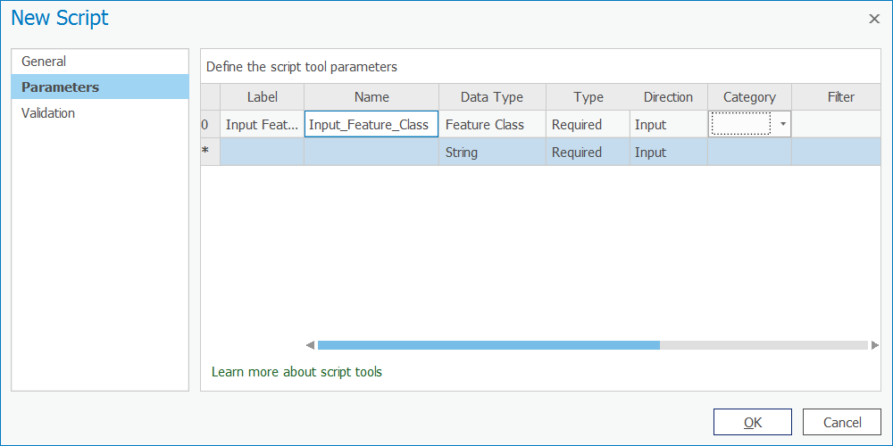 Figure 1.11 Choosing "Feature Class."
 - Just as you did in the previous steps, add a second parameter labeled Output Feature Class. The data type should again be Feature Class.
- For the Output Feature Class parameter, change the Direction property to Output.
- Add a third parameter named Buffer Distance. Choose Linear Unit as the data type. This data type will allow the user of the tool to select both the distance value and the units (for example, miles, kilometers, etc.).
- Set the Buffer Distance parameter's Default property to 5 Miles. (You may need to scroll to the right to see the Default column.) Your dialog should look like what you see below:
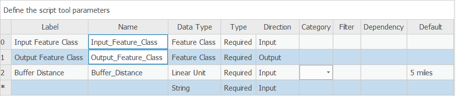 Figure 1.12 Setting the Default property to "5 Miles."
 - Click OK to finish creation of the new script tool and open it by double-clicking it.
- Try out your tool by buffering any feature class on your computer. Notice that once you supply the input feature class, an output feature class path is suggested for you. This is because you specifically set Output Feature Class as an output parameter. Also, when the tool is complete, examine the Details box (visible if you hover your mouse over the tool's "Completed successfully" message) for the custom message "All done!" that you added in your code.
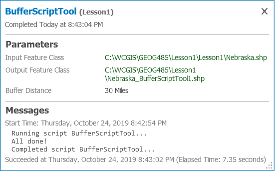 Figure 1.13 The tool is complete.
This is a very simple example, and obviously, you could just run the out-of-the-box Buffer tool with similar results. Normally, when you create a script tool, it will be backed with a script that runs a combination of tools and applies some logic that makes those tools uniquely useful.
There’s another benefit to this example, though. Notice the simplicity of our script tool dialog compared to the main Buffer tool:
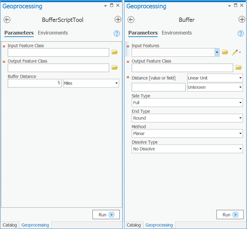
At some point, you may need to design a set of tools for beginning GIS users where only the most necessary parameters are exposed. You may also do this to enforce quality control if you know that some of the parameters must always be set to certain defaults, and you want to avoid the scenario where a beginning user (or a rogue user) might change the required values. A simple script tool is effective for simplifying the tool dialog in this way.
Lesson content developed by Jim Detwiler, Jan Wallgrun and James O’Brien
Adding Tool Validation Code
Now let’s expand on the user friendliness of the tool by using the validator methods to ensure that our cutoff value falls within the minimum and maximum values of our raster (otherwise performing the analysis is a waste of resources).
The purpose of the validation process is to allow us to have some customizable behavior depending on what values we have in our tool parameters. For example, we might want to make sure a value is within a range as in this case (although we could do that within our code as well), or we might want to offer a user different options if they provide a point feature class instead of a polygon feature class, or different options if they select a different type of field (e.g. a string vs. a numeric type).
The Esri help for Tool Validation(link is external) [86] gives a longer list of uses and also explains the difference between internal validation (what Desktop & Pro do for us already) and the validation that we are going to do here which works in concert with that internal validation.
You will notice in the help that Esri specifically tells us not to do what I’m doing in this example – running geoprocessing tools. The reason for this is they generally take a long time to run. In this case, however, we’re using a very simple tool which gets the minimum & maximum raster values and therefore executes very quickly. We wouldn’t want to run an intersection or a buffer operation for example in the ToolValidator, but for something very small and fast such as this value checking, I would argue that it’s ok to break Esri’s rule. You will probably also note that Esri hints that it’s ok to do this by using Describe to get the properties of a feature class and we’re not really doing anything different except we’re getting the properties of a raster.
So how do we do it? Go back to your tool (either in the Toolbox for your Project, Results, or the Recent Tools section of the Geoprocessing sidebar), right click and choose Properties and then Validation.
You will notice that we have a pre-written, Esri-provided class definition here. We will talk about how class definitions look in Python in Lesson 4 but the comments in this code should give you an idea of what the different parts are for. We’ll populate this template with the lines of code that we need. For now, it is sufficient to understand that different methods (initializeParameters(), updateParameters(), etc.) are defined that will be called by the script tool dialog to perform the operations described in the documentation strings following each line starting with def.
Take the code below and use it to overwrite what is in your ToolValidator:
import arcpy
class ToolValidator(object):
"""Class for validating a tool's parameter values and controlling
the behavior of the tool's dialog."""
def __init__(self):
"""Setup arcpy and the list of tool parameters."""
self.params = arcpy.GetParameterInfo()
def initializeParameters(self):
"""Refine the properties of a tool's parameters. This method is
called when the tool is opened."""
def updateParameters(self):
"""Modify the values and properties of parameters before internal
validation is performed. This method is called whenever a parameter
has been changed."""
def updateMessages(self):
"""Modify the messages created by internal validation for each tool
parameter. This method is called after internal validation."""
## Remove any existing messages
self.params[1].clearMessage()
if self.params[1].value is not None:
## Get the raster path/name from the first [0] parameter as text
inRaster1 = self.params[0].valueAsText
## calculate the minimum value of the raster and store in a variable
elevMINResult = arcpy.GetRasterProperties_management(inRaster1, "MINIMUM")
## calculate the maximum value of the raster and store in a variable
elevMAXResult = arcpy.GetRasterProperties_management(inRaster1, "MAXIMUM")
## convert those values to floating points
elevMin = float(elevMINResult.getOutput(0))
elevMax = float(elevMAXResult.getOutput(0))
## calculate a new cutoff value if the original wasn't suitable but only if the user hasn't specified a value.
if self.params[1].value < elevMin or self.params[1].value > elevMax:
cutoffValue = elevMin + ((elevMax-elevMin)/100*90)
self.params[1].value = cutoffValue
self.params[1].setWarningMessage("Cutoff Value was outside the range of ["+str(elevMin)+","+str(elevMax)+"] supplied raster so a 90% value was calculated")
Our logic here is to take the raster supplied by the user and determine the min and max values so that we can evaluate whether the cutoff value supplied by the user falls within that range. If that is not the case, we're going to do a simple mathematical calculation to find the value 90% of the way between the min and max values and suggest that as a default to the user (by putting it into the parameter). We’ll also display a warning message to the user telling them that the value has been adjusted and why their original value doesn’t work.
As you look over the code, you’ll see that all of the work is being done in the bottom function updateMessages(). This function is called after the updateParameters() and the internal arcpy validation code have been executed. It is mainly intended for modifying the warning or error messages produced by the internal validation code. The reason why we are putting all our validation code here is because we want to produce the warning message and there is no entirely simple way to do this if we already perform the validation and potentially automatic adjustment of the cutoff value in updateParameters() instead. Here is what happens in the updateMessages() function:
We start by cleaning up any previous messages self.params[1].clearMessages() (line 24). Then we check if the user has entered a value into the cutoffValue parameter (self.params[1]) on line 26. If they haven't, we don’t do anything (for efficiency). If the user has entered a value (i.e., the value is not None) then we get the raster name from the first parameter (self.params[0]) and we extract it as text (because we want the content to use as a path) on line 28. Then we’ll call the arcpy GetRasterProperties function twice, once to get the min value (line 30) and again to get the max value (on line 32) of the raster. We’ll then convert those values to floating point numbers (lines 34 & 35).
Once we’ve done that, we do a little bit of checking to see if the value the user supplied is within the range of the raster. If it is not, then we will do some simple math to calculate a value that falls 90% of the way into the range and then update the parameter (self.params[1].value) with the number we calculated (line 40 and 41). Finally, in line 42, we produce the warning message informing the users of the automatic value adjustment.
Now let’s test our Validator. Click OK and return to your script in the Toolbox, Results or Geoprocessing window. Run the script again. Insert the name of the input raster again. If you didn’t make any mistakes entering the code there won’t be a red X by the Input Raster. If you did make a mistake, an error message will be displayed there, showing you the usual arcpy / geoprocessing error message and the line of code that the error is occurring on. If you have to do any debugging, exit the script, return to the Toolbox, right click the script and go back to the Tool Validator and correct the error. Repeat as many times as necessary.
If there were no errors, we should test out our validation by putting a value into our Cutoff Value parameter that we know to be outside the range of our data. If you choose a value < 2798 or > 3884, you should see a yellow warning triangle appear that displays our error message, and you will also note that the value in Cutoff Value has been updated to our 90% value.
We can change the value to one we know works within the range (e.g. 3500), and now the tool should run.
Lesson content developed by Jan Wallgrun and James O’Brien
ArcGIS Pro Add-in Introduction
ESRI provides the ability to extend and customize the Pro application through the ArcGIS Pro SDK for .Net [87]. The SDK provides access to much of the Pro application framework to include creating custom ribbon menu’s and buttons, branded configurations, custom geoprocessing ‘add-ins’.
Since each ArcGIS Pro project’s folders, toolboxes, databases, etc.,. is compartmentalized to the project, the user needs to add the custom toolbox with the script tools from the favorites or set the toolbox to be added to new projects. This can get confusing for some users. One benefit of using the SDK and creating Add-ins for the custom geoprocessing tools is the way they are deployed to the user. The add-in is deployed through the addinx through the addin manager. It can be hosted on a network shared folder, installed locally, or hosted for download on the Organizations Portal and is loaded for every project. Instead of running script tool from a toolbox, the tool is loaded from clicking the button on the Ribbon Menu.
Another difference between the add-in and script tool that may be useful for some geoprocessing workflows is the ability to create dynamic interactivity into the add-in and work with features in the mapview. Script tools are linear and require the user input and settings before it is started. You can do some limited interactivity such as extent, selection, and loaded layers but Add-ins can provide the ability to work through the process dynamically. An example might be creating a tool that assists non-gis users the ability to edit attributes through a UI (User Interface) and code tailored to that dataset. You can perform CRUD operations on a table of data while providing the user with informational prompt messages that take user input.
To create the add-in, knowledge of the C# language and WPF (Windows Presentation Format) architecture is needed and is unfortunately beyond the scope of this course. Esri provides instructor led training courses as well as a lot of complete SDK samples (as visual studio projects), code snippets, and tutorials in their SDK documentation and Github repository.
PyQt (overview)
While it’s good and useful to understand how to write Python code to create a GUI directly, it’s obviously a very laborious and time consuming approach that requires writing a lot of code. So together with the advent of early GUI frameworks, people also started to look into more visual approaches in which the GUI of a new software application is clicked and dragged together from predefined building blocks. The typical approach is that first the GUI is created within the graphical GUI building tool and then the tool translates the graphical design into code of the respective programming language that is then included into the main code of the new software application.
Note that this too could be an 8 week course as well and due to time contraints, this is provided as an overview. If you are interested in exploring it more, please view the full topic in the full 10-week course content [89].
Creating GUIs with QT Designer 2.6.2
The GUI building tool for QT that we are going to use in this lesson is called QT Designer. QT Designer is included in the PyQT5 Python package and can be installed through ArcGIS Pro Python Package manager. The tool itself is platform and programming language independent. Instead of producing code from a particular programming language, it creates a .ui file with an xml description of the QT-based GUI. This .ui file can then be translated into Python code with the pyuic5 GUI compiler tool that also comes with PyQT5. There is also support for directly reading the .ui file from Python code in PyQT5 and then generating the GUI from its content, but we here demonstrate the approach of creating the Python code with pyui5 because it is faster and allows us to see and inspect the Python code for our application. In the following, we will take a quick look at how the QT Designer works.
You can install PyQt5 from the ArcGIS Pro package manager. The QT Designer executable will be in your ArcGIS Pro Python environment folder, either under "C:\Users\<username>\AppData\Local\ESRI\conda\envs\arcgispro-py3-clone\Library\bin\designer.exe" or under “C:\Program Files\ArcGIS\Pro\bin\Python\envs\arcgispro-py3\Library\bin\designer.exe”. It might be good idea to create a shortcut to this .exe file on your desktop for the duration of the course, allowing you to directly start the application. After starting, QT Designer will greet you as shown in the figure below:

QT Designer allows for creating so-called “forms” which can be the GUI for a dialog box, a main window, or just a simple QWidget. Each form is saved as a single .ui file. To create a new form, you pick one of the templates listed in the “New Form” dialog. Go ahead and double-click the “Main Window” template. As a result, you will now see an empty main window form in the central area of the QT Designer window.

Let’s quickly go through the main windows of QT Designer. On the left side, you see the “Widget Box” pane that lists all the widgets available including layout widgets and spacers. Adding a widget to the current form can be done by simply dragging the widget from the pane and dropping it somewhere on the form. Go ahead and place a few different widgets like push buttons, labels, and line edits somewhere on the main window form. When you do a right-click in an empty part of the central area of the main window form, you can pick “Lay out” in the context menu that pops up to set the layout that should be used to arrange the child widgets. Do this and pick “Lay out horizontally” which should result in all the widgets you added being arranged in a single row. See what happens if you instead change to a grid or vertical layout. You can change the layout of any widget that contains other widgets in this way.
On the right side of QT Designer, there are three different panes. The one at the top called “Object Inspector” shows you the hierarchy of all the widgets of the current form. This currently should show you that you have a QMainWindow widget with a QWidget for its central area, which in turn has several child widgets, namely the widgets you added to it. You can pretty much perform the same set of operations that are available when interacting with a widget in the form (like changing its layout) with the corresponding entry in the “Object Inspector” hierarchy. You can also drag and drop widgets onto entries in the hierarchy to add new child widgets to these entries, which can sometimes be easier than dropping them on widgets in the form, e.g., when the parent widget is rather small.
The “Object” column lists the object name for each widget in the hierarchy. This name is important because when turning a GUI form into Python code, the object name will become the name of the variable containing that widget. So if you need to access the widget from your main code, you need to know that name and it’s a good idea to give these widgets intuitive names. To change the object name to something that is easier to recognize and remember, you can double-click the name to edit it, or you can use “Change objectName” from the context menu when you right-click on the entry in the hierarchy or the widget itself.
Below the “Object Inspector” window is the “Property Editor”. This shows you all the properties of the currently selected widget and allows you to change them. The yellow area lists properties that all widgets have, while the green and blue areas below it (you may have to scroll down to see these) list special properties of that widget class. For instance, if you select a push button you added to your main window form, you will find a property called “text” in the green area. This property specifies the text that will be displayed on the button. Click on the “Value” column for that property, enter “Push me”, and see how the text displayed on the button in the main window form changes accordingly. Some properties can also be changed by double-clicking the widget in the form. For instance, you can also change the text property of a push button or label by double-clicking it.
If you double-click where it says “Type Here” at the top, you can add a menu to the menu bar of the main window. Give this a try and call the menu “File”.

The last pane on the right side has three tabs below it. “Resource browser” allows for managing additional resources, like files containing icons to be used as part of the GUI. “Action editor” allows for creating actions for your GUI. Remember that actions are for things that can be initiated via different GUI elements. If you click the “New” button at the top, a dialog for creating a new action opens up. You can just type in “test” for the “Text” property and then press “OK”. The new action will now appear as actionTest in the list of actions. You can drag it and drop it on the File menu you created to make this action an entry in that menu.

Finally, the “Signal/Slot Editor” tab allows for connecting signals of the widgets and actions created to slots of other widgets. We will mainly connect signals with event handler functions in our own Python code rather than in QT Designer, but if some widgets’ signals should be directly connected to slots of other widgets this can already be done here.
You now know the main components of QT Designer and a bit about how to place and arrange widgets in a form. We cannot teach QT Designer in detail here but we will show you an example of creating a larger GUI in QT Designer as part of the following first walkthrough of this lesson. If you want to learn more, there exist quite a few videos explaining different aspects of how to use QT Designer on the web. For now, here is a short video (12:21min) that we recommend checking out to see a few more basic examples of the interactions we briefly described above before moving on to the walkthrough.
Video: Qt Designer - PyQt with Python GUI Programming tutorial [90] by sentdex [91]
Once you have created the form(s) for the GUI of your program and saved them as .ui file(s), you can translate them into Python code with the help of the pyuic5 tool, e.g. by running a command like the following from the command line using the tool directly with Python :
"C:\Users\<username>\AppData\Local\ESRI\conda\envs\arcgispro-py3-clone\python.exe" –m PyQt5.uic.pyuic mainwindow.ui –o mainwindow.py
or
"C:\Program Files\ArcGIS\Pro\bin\Python\envs\arcgispro-py3\python.exe" –m PyQt5.uic.pyuic mainwindow.ui –o mainwindow.py
depending on where your default Python environment is located (don't forget to replace <username> with your actual user name in the first version and if you get an error with this command try typing it in, not copying/pasting). mainwindow.ui, here, is the name of the file produced with QT Designer, and what follows the -o is the name of the output file that should be produced with the Python version of the GUI. If you want, you can do this for your own .ui file now and have a quick look at the produced .py file and see whether or not you understand some of the things happening in it. We will demonstrate how to use the produced .py file to create the GUI from your Python code as part of the walkthrough in the next section.
Lesson content developed by Jan Wallgrun and James O’Brien
The QGIS Scripting Interface and Python API 4.5
Interacting with Layers Open in QGIS 4.5.1
Let us start this introduction by writing some code directly in the QGIS Python console and talking about how you can access the layers currently open in QGIS and add new layers to the currently open project. If you don’t have QGIS running at the moment, please start it up and open the Python console from the Plugins menu in the main menu bar.
When you open the Python console in QGIS, the Python qgis package and its submodules are automatically imported as well as other relevant modules including the main PyQt5 modules. In addition, a variable called iface is set up to provide an object of the class QgisInterface1 [92] to interact with the running QGIS environment. The code below shows how you can use that object to retrieve a list of the layers in the currently open map project and the currently active layer. Before you type in and run the code in the console, please add a few layers to an empty project including the TM_WORLD_BORDERS-0.3.shp shapefile (download here) [93]. We will recreate some of the steps from that section with QGIS here so that you also get a bit of a comparison between the two APIs (Application Programming Interfaces). The currently active layer is the one selected in the Layers window; please select the world borders layer by clicking on it before you execute the code.
layers = iface.mapCanvas().layers()
for layer in layers:
print(layer)
print(layer.name())
print(layer.id())
print('------')
# If you copy/paste the code - run the part above
# before you run the part below
# otherwise you'll get a syntax error.
activeLayer = iface.activeLayer()
print('active layer: ' + activeLayer.name())
Output (numbers will vary): ...TM_WORLD_BORDERS-0.3 TM_WORLD_BORDERS_0_3_2e5a7cd5_591a_4d45_a4aa_cbba2e639e75 ------ ... active layer: TM_WORLD_BORDERS-0.3
The layers() method of the QgsMapCanvas [94] object we get from calling iface.mapCanvas() returns the currently open layers as a list of objects of the different subclasses of QgsMapLayer [95]. Invoking the name() method of these layer objects gives us the name under which the layer is listed in the Layers window. layer.id() gives us the ID that QGIS has assigned to the layer which in contrast to the name is unique. The iface.activeLayer() method gives us the currently selected layer.
The type() function of a layer can be used to test the type of the layer:
if activeLayer.type() == QgsMapLayer.VectorLayer:
print('This is a vector layer!')
Depending on the type of the layer, there are other methods that we can call to get more information about the layer. For instance, for a vector layer [96] we can use wkbType() to get the geometry type of the layer:
if activeLayer.type() == QgsMapLayer.VectorLayer:
if activeLayer.wkbType() == QgsWkbTypes.MultiPolygon:
print('This layer contains multi-polygons!')
The output you get from the previous command should confirm that the active world borders layer contains multi-polygons, meaning features that can have multiple polygonal parts.
QGIS defines a function dir(…) that can be used to list the methods that can be invoked for a given object. Try out the following two applications of this function:
dir(iface) dir(activeLayer)
To add or remove a layer, we need to work with the QgsProject [97] object for the project currently open in QGIS. We retrieve it like this:
currentProject = QgsProject.instance() print(currentProject.fileName())
The output from the print statement in the second row will probably be the empty string unless you have saved the project. Feel free to do so and rerun the line and you should get the actual file name.
Here is how we can remove the active layer (or any other layer object) from the layer registry of the project (you may have to resize/refresh the map canvas afterwards for the layer to disappear there):
currentProject.removeMapLayer(activeLayer.id())
The following command shows how we can add the world borders shapefile again (or any other feature class we have on disk). Make sure you adapt the path based on where you have the shapefile stored. We first have to create the vector layer object providing the file name and optionally the name to be used for the layer. Then we add that layer object to the project via the addMapLayer(…) method:
layer = QgsVectorLayer(r'C:\489\TM_WORLD_BORDERS-0.3.shp', 'World borders') currentProject.addMapLayer(layer)
Lastly, here is an example that shows you how you can change the symbology of a layer from your code:
renderer = QgsGraduatedSymbolRenderer()
renderer.setClassAttribute('POP2005')
layer.setRenderer(renderer)
layer.renderer().updateClasses(layer, QgsGraduatedSymbolRenderer.Jenks, 5)
layer.renderer().updateColorRamp(QgsGradientColorRamp(Qt.white, Qt.red))
iface.layerTreeView().refreshLayerSymbology(layer.id())
iface.mapCanvas().refreshAllLayers()
Here we create an object of the QgsGraduatedSymbolRenderer class that we want to use to draw the country polygons from our layer using a graduated color approach based on the population attribute ‘POP2005’. The name of the field to use is set via the renderer’s setClassAttribute() method in line 2. Then we make the renderer object the renderer for our world borders layer in line 3. In the next two lines, we tell the renderer (now accessed via the layer method renderer()) to use a Jenks Natural Breaks classification with 5 classes and a gradient color ramp that interpolates between the colors white and red. Please note that the colors used as parameters here are predefined instances of the Qt5 class QColor. Changing the symbology does not automatically refresh the map canvas or layer list. Therefore, in the last two lines, we explicitly tell the running QGIS environment to refresh the symbology of the world borders layer in the Layers tree view (line 6) and to refresh the map canvas (line 7). The result should look similar to the figure below (with all other layers removed).

[1] The qgis Python module is a wrapper around the underlying C++ library. The documentation pages linked in this section are those of the C++ version but the names of classes and available functions and methods are the same.
Lesson content developed by Jan Wallgrun and James O’Brien
Accessing the Features of a Layer
Let’s keep working with the world borders layer open in QGIS for a bit, looking at how we can access the individual features in a layer and select features by attribute. The following piece of code shows you how we can loop through all the features with the help of the layer’s getFeatures() method:
for feature in layer.getFeatures():
print(feature)
print(feature.id())
print(feature['NAME'])
print('-----')
Output: <qgis._core.QgsFeature object at 0x...> 0 Antigua and Barbuda ----- <qgis._core.QgsFeature object at 0x...> 1 Algeria ----- <qgis._core.QgsFeature object at 0x...> 2 Azerbaijan ----- <qgis._core.QgsFeature object at 0x...> 3 Albania ----- ...
Features are represented as objects of the class QgsFeature(link is external) [98] in QGIS. So, for each iteration of the for-loop in the previous code example, variable feature will contain a QgsFeature object. Features are numbered with a unique ID that you can obtain by calling the method id() as we are doing in this example. Attributes like the NAME attribute of the world borders polygons can be accessed using the attribute name as the key as also demonstrated above.
Like in most GIS software, a layer can have an active selection. When the layer is open in QGIS, the selected features are highlighted. The layer method selectAll() allows for selecting all features in a layer and removeSelection() can be used to clear the selection. Give this a try by running the following two commands in the QGIS Python console and watch how all countries become selected and then deselected again.
layer.selectAll() layer.removeSelection()
The method selectByExpression() allows for selecting features based on their properties with a SQL query string that has the same format as in ArcGIS. Use the following command to select all features from the layer that have a value larger than 300,000 in the AREA column of the attribute table. The result should look as in the figure below.
layer.selectByExpression('"AREA" > 300000')

While there can only be one active selection for a layer, you can create as many subgroups of features from a layer as you want by calling getFeatures(…) with a parameter that is an object of the class QgsFeatureRequest [99] and that has been given a filter expression via its setFilterExpression(…) method. The filter expression can be again an SQL query string. The following code creates a subgroup that will only contain the polygon for Canada. When you run it, this will not change the active selection that you see for that layer in QGIS but variable selectionName now provides access to the subgroup with just that one polygon. We get that first (and only) polygon by calling the __next__() method of selectionName and then print out some information about this particular polygon feature.
selectionName = layer.getFeatures(QgsFeatureRequest().setFilterExpression('"NAME" = \'Canada\''))
feature = selectionName.__next__()
print(feature['NAME'] + "-" + str(feature.id()))
print(feature.geometry())
print(feature.geometry().asWkt())
Output: Canada – 23 <qgis._core.QgsGeometry object at 0x...> MultiPolygon (((-65.61361699999997654 43.42027300000000878,...)))
The first print statement in this example works in the same way as you have seen before to get the name attribute and id of the feature. The method geometry() gives us the geometric object for this feature as an instance of the QgsGeometry class [100] and calling the method asWkt() gives us a WKT string representation of the multi-polygon geometry. You can also use a for-loop to iterate through the features in a subgroup created in this way. The method rewind() can be used to reset the iterator to the beginning so that when you call __next__() again, it will again give you the first feature from the subgroup.
When you have the geometry object and know what type of geometry it is, you can use the methods asPoint(), asPolygon(), asPolyline(), asMultiPolygon(), etc. to get the geometry as a Python data structure, e.g. in the case of multi-polygons as a list of lists of lists with each inner list containing tuples of the point coordinates for one polygonal component.
print(feature.geometry().asMultiPolygon())
[[[(-65.6136, 43.4203), (-65.6197,43.4181), … ]]]
Here is another example to demonstrate that we can work with several different subgroups of features at the same time. This time we request all features from the layer that have a POP2005 value larger than 50,000,000.
selectionPopulation = layer.getFeatures(QgsFeatureRequest().setFilterExpression('"POP2005" > 50000000'))
If we ever want to use a subgroup like this to create the active selection for the layer from it, we can use the layer method selectByIds(…) for this. The method requires a list of feature IDs and will then change the active selection to these features. In the following example, we use a simple list comprehension to create the ID list from the subgroup in our variable selectionPopulation:
layer.selectByIds([f.id() for f in selectionPopulation])
When running this command you should notice that the selection of the features in QGIS changes to look like in the figure below.

Let’s save the currently selected features as a new file. We use the GeoPackage format (GPKG) for this, which is more modern than the shapefile format, but you can easily change the command below to produce a shapefile instead; simply change the file extension to “.shp” and replace “GPKG” with “ESRI Shapefile”. The function we will use for writing the layer to disk is called writeAsVectorFormat(…) and it is defined in the class QgsVectorFileWriter [101]. Please note that this function has been declared "deprecated", meaning it may be removed in future versions and it is recommended that you do not use it anymore. In versions up to QGIS 3.16 (the current LTR version that most likely you are using right now), you are supposed to use writeAsVectorFormatV2(...) instead; however, there have been issues reported with that function and it is already replaced by writeAsVectorFormatV3(...) in versions >3.16 of QGIS. Therefore, we have decided to stick with writeAsVectorFormat(…) while things are still in flux. The parameters we give to writeAsVectorFormat(…) are the layer we want to save, the name of the output file, the character encoding to use, the spatial reference to use (we simply use the one that our layer is in), the format (“GPKG”), and True for signaling that only the selected features should be saved in the new data set. Adapt the path for the output file as you see fit and then run the command:
QgsVectorFileWriter.writeAsVectorFormat(layer, r'C:\489\highPopulationCountries.gpkg', 'utf-8', layer.crs(),'GPKG', True)
If you add the new file produced by this command to your QGIS project, it should only contain the polygons for the countries we selected based on their population values.
For changing the attribute values of a feature, we need to work with the “data provider” object of the layer. We can access it via the layer’s dataProvider() method:
dataProvider = layer.dataProvider()
Let’s say we want to change the POP2005 value for Canada to 1 (don’t ask what happened!). For this, we also need the index of the POP2005 column which we can get by calling the data provider’s fieldNameIndex() method:
populationColumnIndex = dataProvider.fieldNameIndex('POP2005')
To change the attribute value we call the method changeAttributeValues(…) of the data provider object providing a dictionary as parameter that maps feature IDs to dictionaries which in turn map column indices to new values. The inner dictionary that maps column indices to values is defined in a separate variable newValueDictionary.
newValueDictionary = { populationColumnIndex : 1 }
dataProvider.changeAttributeValues( { feature.id(): newValueDictionary } )
In this simple example, the outer dictionary contains only a single key-value pair with the ID of the feature for Canada as key and another dictionary as value. The inner dictionary also only contains a single key-value pair consisting of the index of the population column and its new value 1. Both dictionaries can have multiple entries to simultaneously change multiple values of multiple features. After running this command, check out the attributes of Canada, either via the QGIS Identify tool or in the attribute table of the layer. You will see that the population value in the layer now has been changed to 1 (the same holds for the underlying shapefile). Let’s set the value back to what it was with the following command:
dataProvider.changeAttributeValues( { feature.id(): { populationColumnIndex : 32270507 } } )
Lesson content developed by Jan Wallgrun and James O’Brien
Creating Features and Geometric Operations
Let us switch from the Python console in QGIS to writing a standalone script that uses qgis. You can use your editor of choice to write the script and then execute the .py file from the OSGeo4W shell with all environment variables set correctly for a qgis and QT5 based program.
We are going to create buffers around the centroids of the countries within a rectangular (in terms of WGS 84 coordinates) area around southern Africa using the TM_WORLD_BORDERS data (download) [84]. We will produce two new vector GeoPackage files: a point based one with the centroids and a polygon based one for the buffers. Both data sets will only contain the country name as their only attribute.
We start by importing the modules we will need and creating a QApplication() (handled by qgis.core.QgsApplication) for our program that qgis can run in (even though the program does not involve any GUI).
Important note: When you later write you own qgis programs, make sure that you always "import qgis" first before using any other qgis related import statements such as "import qgis.core". The qgis package needs to be loaded and 'started' (handled by the underlying code with qgis) or other imports will most likely fail tend to fail without "import qgis" coming first.
import os, sys import qgis import qgis.core
To use qgis in our software, we have to initialize it and we need to tell it where the actual QGIS installation is located. To do this, we use the function getenv(…) of the os module to get the value of the environmental variable “QGIS_PREFIX_PATH” which will be correctly defined when we run the program from the OSGeo4W shell. Then we create an instance of the QgsApplication class and call its initQgis() method.
qgis_prefix = os.getenv("QGIS_PREFIX_PATH")
qgis.core.QgsApplication.setPrefixPath(qgis_prefix, True)
qgs = qgis.core.QgsApplication([], False)
qgs.initQgis()
Now we can implement the main functionality of our program. First, we load the world borders shapefile into a layer (you may have to adapt the path!).
layer = qgis.core.QgsVectorLayer(r'C:\489\TM_WORLD_BORDERS-0.3.shp')
Then we create the two new layers for the centroids and buffers. These layers will be created as new in-memory layers and later written to GeoPackage files. We provide three parameters to QgsVectorLayer(…): (1) a string that specifies the geometry type, coordinate system, and fields for the new layer; (2) a name for the layer; and (3) the string “memory” which tells the function that it should create a new layer in memory from scratch (rather than reading a data set from somewhere else as we did earlier).
centroidLayer = qgis.core.QgsVectorLayer("Point?crs=" + layer.crs().authid() + "&field=NAME:string(255)", "temporary_points", "memory")
bufferLayer = qgis.core.QgsVectorLayer("Polygon?crs=" + layer.crs().authid() + "&field=NAME:string(255)", "temporary_buffers", "memory")
The strings produced for the first parameters will look like this: “Point?crs=EPSG:4326&field=NAME:string(255)” and “Polygon?crs=EPSG:4326&field=NAME:string(255)”. Note how we are getting the EPSG string from the world border layer so that the new layers use the same coordinate system, and how an attribute field is described using the syntax “field=<name of the field>:<type of the field>". When you want your layer to have more fields, these have to be separated by additional & symbols like in a URL (Universal Resource Locators).
Next, we set up variables for the data providers of both layers that we will need to create new features for them. The new features will be collected in two lists, centroidFeatures and bufferFeatures.
centroidProvider = centroidLayer.dataProvider() bufferProvider = bufferLayer.dataProvider() centroidFeatures = [] bufferFeatures = []
Then, we create the polygon geometry for our selection area from a WKT string as in Section 3.9.1:
areaPolygon = qgis.core.QgsGeometry.fromWkt('POLYGON ( (6.3 -14, 52 -14, 52 -40, 6.3 -40, 6.3 -14) )')
In the main loop of our program, we go through all the features in the world borders layer, use the geometry method intersects(…) to test whether the country polygon intersects with the area polygon, and, if yes, create the centroid and buffer features for the two layers from the input feature.
for feature in layer.getFeatures():
if feature.geometry().intersects(areaPolygon):
centroid = qgis.core.QgsFeature()
centroid.setAttributes([feature['NAME']])
centroid.setGeometry(feature.geometry().centroid())
centroidFeatures.append(centroid)
buffer = qgis.core.QgsFeature()
buffer.setAttributes([feature['NAME']])
buffer.setGeometry(feature.geometry().centroid().buffer(2.0,100))
bufferFeatures.append(buffer)
Note how in both cases (centroids and buffers), we first create a new QgsFeature object, then use setAttributes(…) to set the NAME attribute to the name of the country, and then use setGeometry(…) to set the geometry of the new feature either to the centroid derived by calling the centroid() method or to the buffered centroid created by calling the buffer(…) method of the centroid point. As a last step, the new features are added to the respective lists. Finally, all features in the two lists are added to the layers after the for-loop has been completed. This happens with the following two commands:
centroidProvider.addFeatures(centroidFeatures) bufferProvider.addFeatures(bufferFeatures)
Lastly, we write the content of the two in-memory layers to GeoPackage files on disk. This works in the same way as in previous examples. Again, you might want to adapt the output paths.
qgis.core.QgsVectorFileWriter.writeAsVectorFormat(centroidLayer, r'C:\489\centroids.gpkg', "utf-8", layer.crs(), "GPKG") qgis.core.QgsVectorFileWriter.writeAsVectorFormat(bufferLayer, r'C:\489\buffers.gpkg', "utf-8", layer.crs(), "GPKG")
Since we are now done with using QGIS functionalities (and actually the entire program), we clean up by calling the exitQgis() method of the QgsApplication, freeing up resources that we don’t need anymore.
qgs.exitQgis()
If you run the program from the OSGeo4W shell and then open the two produced output files in QGIS, the result should look as shown in the image below.

Lesson content developed by Jan Wallgrun and James O’Brien
Working with raster data
OGR and GDAL exist as separate modules in the osgeo package together with some other modules such as OSR for dealing with different projections and some auxiliary modules. As with previous packages you will probably need to install gdal (which encapsulates all of them in its latest release) to access these packages. So typically, a Python project using GDAL would import the needed modules similar to this:
raster = gdal.Open(r'c:\489\L3\wc2.0_bio_10m_01.tif')
To open an existing raster file in GDAL, you would use the Open(...) function defined in the gdal module. The raster file we will use in the following examples contains world-wide bioclimatic data and will be used again in the lesson’s walkthrough. Download the raster file here [102].
raster.RasterCount
We now have a GDAL raster dataset in variable raster. Raster datasets are organized into bands. The following command shows that our raster only has a single band:
raster.RasterCount
Output: 1
To access one of the bands, we can use the GetRasterBand(...) method of a raster dataset and provide the number of the band as a parameter (counting from 1, not from 0!):
band = raster.GetRasterBand(1) # get first band of the raster
If your raster has multiple bands and you want to perform the same operations for each band, you would typically use a for-loop to go through the bands:
for i in range(1, raster.RasterCount + 1):
b = raster.GetRasterBand(i)
print(b.GetMetadata()) # or do something else with b
There are a number of methods to read different properties of a band in addition to GetMetadata() used in the previous example, such as GetNoDataValue(), GetMinimum(), GetMaximum(), andGetScale().
print(band.GetNoDataValue()) print(band.GetMinimum()) print(band.GetMaximum()) print(band.GetScale())
Output: -1.7e+308 -53.702073097229 33.260635217031 1.0
GDAL provides a number of operations that can be employed to create new files from bands. For instance, the gdal.Polygonize(...) function can be used to create a vector dataset from a raster band by forming polygons from adjacent cells that have the same value. To apply the function, we first create a new vector dataset and layer in it. Then we add a new field ‘DN’ to the layer for storing the raster values for each of the polygons created:
drv = ogr.GetDriverByName('ESRI Shapefile')
outfile = drv.CreateDataSource(r'c:\489\L3\polygonizedRaster.shp')
outlayer = outfile.CreateLayer('polygonized raster', srs = None )
newField = ogr.FieldDefn('DN', ogr.OFTReal)
outlayer.CreateField(newField)
Once the shapefile is prepared, we call Polygonize(...) and provide the band and the output layer as parameters plus a few additional parameters needed:
gdal.Polygonize(band, None, outlayer, 0, []) outfile = None
With the None for the second parameter we say that we don’t want to provide a mask for the operation. The 0 for the fourth parameter is the index of the field to which the raster values shall be written, so the index of the newly added ‘DN’ field in this case. The last parameter allows for passing additional options to the function but we do not make use of this, so we provide an empty list. The second line "outfile = None" is for closing the new shapefile and making sure that all data has been written to it. The result produced in the new shapefile rasterPolygonized.shp should look similar to the image below when looked at in a GIS and using a classified symbology based on the values in the ‘DN’ field.

Polygonize(...) is an example of a GDAL function that operates on an individual band. GDAL also provides functions for manipulating raster files directly, such as gdal.Translate(...) for converting a raster file into a new raster file. Translate(...) is very powerful with many parameters and can be used to clip, resample, and rescale the raster as well as convert the raster into a different file format. You will see an example of Translate(...) being applied in the lesson’s walkthrough. gdal.Warp(...) is another powerful function that can be used for reprojecting and mosaicking raster files.
While the functions mentioned above and similar functions available in GDAL cover many of the standard manipulation and conversion operations commonly used with raster data, there are cases where one directly wants to work with the values in the raster, e.g. by applying raster algebra operations. The approach to do this with GDAL is to first read the data of a band into a GDAL multi-dimensional array object with the ReadAsArray() method, then manipulate the values in the array, and finally write the new values back to the band with the WriteArray() method.
data = band.ReadAsArray() data
If you look at the output of this code, you will see that the array in variable data essentially contains the values of the raster cells organized into rows. We can now apply a simple mathematical expression to each of the cells, like this:
data = data * 0.1 data
The meaning of this expression is to create a new array by multiplying each cell value with 0.1. You should notice the change in the output from +308 to +307. The following expression can be used to change all values that are smaller than 0 to 0:
print(data.min()) data [ data < 0 ] = 0 print(data.min())
data.min() in the previous example is used to get the minimum value over all cells and show how this changes to 0 after executing the second line. Similarly to what you saw with pandas data frames in Section 3.8.6, an expression like data < 0 results in a Boolean array with True for only those cells for which the condition <0 is true. Then this Boolean array is used to select only specific cells from the array with data[...] and only these will be changed to 0. Now, to finally write the modified values back to a raster band, we can use the WriteArray(...) method. The following code shows how one can first create a copy of a raster with the same properties as the original raster file and then use the modified data to overwrite the band in this new copy:
drv = gdal.GetDriverByName('GTiff') # create driver for writing geotiff file
outRaster = drv.CreateCopy(r'c:\489\newRaster.tif', raster , 0 ) # create new copy of inut raster on disk
newBand = outRaster.GetRasterBand(1) # get the first (and only) band of the new copy
newBand.WriteArray(data) # write array data to this band
outRaster = None # write all changes to disk and close file
This approach will not change the original raster file on disk. Instead of writing the updated array to a band of a new file on disk, we can also work with an in-memory copy instead, e.g. to then use this modified band in other GDAL operations such as Polygonize(...) . An example of this approach will be shown in the walkthrough of this lesson. Here is how you would create the in-memory copy combining the driver creation and raster copying into a single line:
tmpRaster = gdal.GetDriverByName('MEM').CreateCopy('', raster, 0) # create in-memory copy
The approach of using raster algebra operations shown above can be used to perform many operations such as reclassification and normalization of a raster. More complex operations like neighborhood/zonal based operators can be implemented by looping through the array and adapting cell values based on the values of adjacent cells. In the lesson’s walkthrough you will get to see an example of how a simple reclassification can be realized using expressions similar to what you saw in this section.
While the GDAL Python package allows for realizing the most common vector and raster operations, it is probably fair to say that it is not the most easy-to-use software API. While the GDAL Python cookbook(link is external) [103] contains many application examples, it can sometimes take a lot of search on the web to figure out some of the details of how to apply a method or function correctly. Of course, GDAL has the main advantage of being completely free, available for pretty much all main operating systems and programming languages, and not tied to any other GIS or web platform. In contrast, the Esri ArcGIS API for Python discussed in the next section may be more modern, directly developed specifically for Python, and have more to offer in terms of visualization and high-level geoprocessing and analysis functions, but it is tied to Esri’s web platforms and some of the features require an organizational account to be used. These are aspects that need to be considered when making a choice on which API to use for a particular project. In addition, the functionality provided by both APIs only overlaps partially and, as a result, there are also merits in combining the APIs as we will do later on in the lesson’s walkthrough.
Lesson content developed by Jan Wallgrun and James O’Brien
Working with vector data
OGR and GDAL exist as separate modules in the osgeo package together with some other modules such as OSR for dealing with different projections and some auxiliary modules. As with previous packages you will probably need to install gdal (which encapsulates all of them in its latest release) to access these packages. So typically, a Python project using GDAL would import the needed modules similar to this:
from osgeo import gdal from osgeo import ogr from osgeo import osr
Let’s start with taking a closer look at the ogr module for working with vector data. The following code, for instance, illustrates how one would open an existing vector data set, in this case an Esri shapefile. OGR uses so-called drivers to access files in different formats, so the important thing to note is how we first obtain a driver object for ‘ESRI Shapefile’ with GetDriverByName(...) and then use that to open the shapefile with the Open(...) method of the driver object. The shapefile we are using [93] in this example is a file with polygons for all countries in the world (available here) [104] and we will use it again in the lesson’s walkthrough. When you download it, you may still have to adapt the path in the first line of the code below.
shapefile = r'C:\489\L3\TM_WORLD_BORDERS-0.3.shp'
drv =ogr.GetDriverByName('ESRI Shapefile')
dataSet = drv.Open(shapefile)
dataSet now provides access to the data in the shapefile as layers, in this case just a single layer, that can be accessed with the GetLayer(...) method. We then use the resulting layer object to get the definitions of the fields with GetLayerDefn(), loop through the fields with the help of GetFieldCount() and GetFieldDefn(), and then print out the field names with GetName():
layer = dataSet.GetLayer(0)
layerDefinition = layer.GetLayerDefn()
for i in range(layerDefinition.GetFieldCount()):
print(layerDefinition.GetFieldDefn(i).GetName())
Output: FIPS ISO2 ISO3 UN NAME ... LAT
If you want to loop through the features in a layer, e.g., to read or modify their attribute values, you can use a simple for-loop and the GetField(...) method of features. It’s important that, if you want to be able to iterate through the features another time, you have to call the ResetReading() method of the layer after the loop. The following loop prints out the values of the ‘NAME’ field for all features:
for feature in layer:
print(feature.GetField('NAME'))
layer.ResetReading()
Output: Antigua and Barbuda Algeria Azerbaijan Albania ....
We can extend the previous example to also access the geometry of the feature via the GetGeometryRef() method. Here we use this approach to get the centroid of each country polygon (method Centroid()) and then print it out in readable form with the help of the ExportToWkt() method. The output will be the same list of country names as before but this time, each followed by the coordinates of the respective centroid.
for feature in layer:
print(feature.GetField('NAME') + '–' + feature.GetGeometryRef().Centroid().ExportToWkt())
layer.ResetReading()
We can also filter vector layers by attribute and spatially. The following example uses SetAttributeFilter(...) to only get features with a population (field ‘POP2005’) larger than one hundred million.
layer.SetAttributeFilter('POP2005 > 100000000')
for feature in layer:
print(feature.GetField('NAME'))
layer.ResetReading()
Output: Brazil China India ...
We can remove the selection by calling SetAttributeFilter(...) with the empty string:
layer.SetAttributeFilter('')
The following example uses SetSpatialFilter(...) to only get countries overlapping a given polygonal area, in this case an area that covers the southern part of Africa. We first create the polygon via the CreateGeometryFromWkt(...) function that creates geometry objects from Well-Known Text (WKT) strings(link is external) [105]. Then we apply the filter and use a for-loop again to print the selected features:
wkt = 'POLYGON ( (6.3 -14, 52 -14, 52 -40, 6.3 -40, 6.3 -14))' # WKT polygon string for a rectangular area
geom = ogr.CreateGeometryFromWkt(wkt)
layer.SetSpatialFilter(geom)
for feature in layer:
print(feature.GetField('NAME'))
layer.ResetReading()
Output: Angola Madagascar Mozambique ... Zimbabwe
Access to all features and their geometries together with the geometric operations provided by GDAL allows for writing code that realizes geoprocessing operations and other analyses on one or several input files and for creating new output files with the results. To show one example, the following code takes our selection of countries from southern Africa and then creates 2 decimal degree buffers around the centroids of each country. The resulting buffers are written to a new shapefile called centroidbuffers.shp. We add two fields to the newly produced buffered centroids shapefile, one with the name of the country and one with the population, copying over the corresponding field values from the input country file. When you will later have to use GDAL in one of the parts of the lesson's homework assignment, you can use the same order of operations, just with different parameters and input values.
To achieve this task, we first create a spatial reference object for EPSG:4326 that will be needed to create the layer in the new shapefile. Then the shapefile is generated with the shapefile driver object we obtained earlier, and the CreateDataSource(...) method. A new layer inside this shapefile is created via CreateLayer(...) and by providing the spatial reference object as a parameter. We then create the two fields for storing the country names and population numbers with the function FieldDefn(...) and add them to the created layer with the CreateField(...) method using the field objects as parameters. When adding new fields, make sure that the name you provide is not longer than 8 characters or GDAL/OGR will automatically truncate the name. Finally, we need the field definitions of the layer available via GetLayerDefn() to be able to later add new features to the output shapefile. The result is stored in variable featureDefn.
sr = osr.SpatialReference() # create spatial reference object
sr.ImportFromEPSG(4326) # set it to EPSG:4326
outfile = drv.CreateDataSource(r'C:\489\L3\centroidbuffers.shp') # create new shapefile
outlayer = outfile.CreateLayer('centroidbuffers', geom_type=ogr.wkbPolygon, srs=sr) # create new layer in the shapefile
nameField = ogr.FieldDefn('Name', ogr.OFTString) # create new field of type string called Name to store the country names
outlayer.CreateField(nameField) # add this new field to the output layer
popField = ogr.FieldDefn('Population', ogr.OFTInteger) # create new field of type integer called Population to store the population numbers
outlayer.CreateField(popField) # add this new field to the output layer
featureDefn = outlayer.GetLayerDefn() # get field definitions
Now that we have prepared the new output shapefile and layer, we can loop through our selected features in the input layer in variable layer, get the geometry of each feature, produce a new geometry by taking its centroid and then calling the Buffer(...) method, and finally create a new feature from the resulting geometry within our output layer.
for feature in layer: # loop through selected features
ingeom = feature.GetGeometryRef() # get geometry of feature from the input layer
outgeom = ingeom.Centroid().Buffer(2.0) # buffer centroid of ingeom
outFeature = ogr.Feature(featureDefn) # create a new feature
outFeature.SetGeometry(outgeom) # set its geometry to outgeom
outFeature.SetField('Name', feature.GetField('NAME')) # set the feature's Name field to the NAME value of the input feature
outFeature.SetField('Population', feature.GetField('POP2005')) # set the feature's Population field to the POP2005 value of the input feature
outlayer.CreateFeature(outFeature) # finally add the new output feature to outlayer
outFeature = None
layer.ResetReading()
outfile = None # close output file
The final line “outfile = None” is needed because otherwise the file would remain open for further writing and we couldn’t inspect it in a different program. If you open the centroidbuffers.shp shapefile and the country borders shapefile in a GIS of your choice, the result should look similar to the image below. If you check out the attribute table, you should see the Name and Populations columns we created populated with values copied over from the input features.

Centroid() and Buffer() are just two examples of the many availabe methods for producing a new geometry in GDAL. In this lesson's homework assignment, you will instead have to use the ogr.CreateGeometryFromWkt(...) function that we used earlier in this section to create a clip polygon from a WKT string representation but, apart from that, the order of operations for creating the output feature will be the same. The GDAL/OGR cookbook(link is external) [106] contains many Python examples for working with vector data with GDAL, including how to create different kinds of geometries(link is external) [107] from different input formats, calculating envelopes, lengths and areas of a geometry(link is external) [108], and intersecting and combining geometries(link is external) [109]. We recommend that you take a bit of time to browse through these online examples to get a better idea of what is possible. Then we move on to have a look at raster manipulation with GDAL.
Lesson content developed by Jan Wallgrun and James O’Brien
(Geo)processing
QGIS has a toolbox system and visual workflow building component somewhat similar to ArcGIS and its Model Builder. It is called the QGIS processing framework [110] and comes in the form of a plugin called Processing that is installed by default. You can access it via the Processing menu in the main menu bar. All algorithms from the processing framework are available in Python via a QGIS module called processing. They can be combined to solve larger analysis tasks in Python and can also be used in combination with the other qgis methods discussed in the previous sections.
We can get a list of all processing algorithms currently registered with QGIS with the command QgsApplication.processingRegistry().algorithms(). Each processing object in the returned list has an identifying name that you can get via its id() method. The following command, which you can try out in the QGIS Python console, uses this approach to print the names of all algorithms that contain the word “clip”:
[x.id() for x in QgsApplication.processingRegistry().algorithms() if "clip" in x.id()]
Output: ['gdal:cliprasterbyextent', 'gdal:cliprasterbymasklayer','gdal:clipvectorbyextent', 'gdal:clipvectorbypolygon', 'native:clip', 'saga:clippointswithpolygons', 'saga:cliprasterwithpolygon', 'saga:polygonclipping']
As you can see, there are processing versions of algorithms coming from different sources, e.g. natively built into QGIS vs. algorithms based on GDAL (Geospatial Data Abstraction Library). The function algorithmHelp(…) allows you to get some documentation on an algorithm and its parameters. Try it out with the following command:
processing.algorithmHelp("native:clip")
To run a processing algorithm, you have to use the run(…) function and provide two parameters: the id of the algorithm and a dictionary that contains the parameters for the algorithm as key-value pairs. run(…) returns a dictionary with all output parameters of the algorithm. The following example illustrates how processing algorithms can be used to solve the task of clipping a points of interest shapefile to the area of El Salvador, reusing the two data sets from homework assignment 2 (Section 2.10). This example is intended to be run as a standalone program again and most of the code is required to set up the QGIS environment needed, including initializing the Processing environment.
The start of the script looks like in the example from the previous section:
import os,sys
import qgis
import qgis.core
qgis_prefix = os.getenv("QGIS_PREFIX_PATH")
qgis.core.QgsApplication.setPrefixPath(qgis_prefix, True
qgs = qgis.core.QgsApplication([], False)
qgs.initQgis()
After, creating the QGIS environment, we can now initialize the processing framework. To be able to import the processing module we have to make sure that the plugins folder is part of the system path; we do this directly from our code. After importing processing, we have to initialize the Processing environment and we also add the native QGIS algorithms to the processing algorithm registry.
# Be sure to change the path to point to where your plugins folder is located # it may not be the same as this one. sys.path.append(r"C:\OSGeo4W\apps\qgis-ltr\python\plugins") import processing from processing.core.Processing import Processing Processing.initialize() qgis.core.QgsApplication.processingRegistry().addProvider(qgis.analysis.QgsNativeAlgorithms())
Next, we create input variables for all files involved, including the output files we will produce, one with the selected country and one with only the POIs (Points of Interest) in that country. We also set up input variables for the name of the country and the field that contains the country names.
poiFile = r'C:\489\L2\assignment\OSMpoints.shp' countryFile = r'C:\489\L2\assignment\countries.shp' pointOutputFile = r'C:\489\L2\assignment\pointsInCountry.shp' countryOutputFile = r'C:\489\L2\assignment\singleCountry.shp' nameField = "NAME" countryName = "El Salvador"
Now comes the part in which we actually run algorithms from the processing framework. First, we use the qgis:extractbyattribute algorithm to create a new shapefile with only those features from the country data set that satisfy a particular attribute query. In the dictionary with the input parameters for the algorithm, we specify the name of the input file (“INPUT”), the name of the query field (“FIELD”), the comparison operator for the query (0 here stands for “equal”), and the value to which we are comparing (“VALUE”). Since the output will be written to a new shapefile, we do not really need the output dictionary that we get back from calling run(…) but the print statement shows how this dictionary in this case contains the name of the output file under the key “OUTPUT”.
output = processing.run("qgis:extractbyattribute", { "INPUT": countryFile, "FIELD": nameField, "OPERATOR": 0, "VALUE": countryName, "OUTPUT": countryOutputFile })
print(output['OUTPUT'])
To perform the clip operation with the new shapefile from the previous step, we use the “native:clip” algorithm. The input paramters are the input file (“INPUT”), the clip file (“OVERLAY”), and the output file (“OUTPUT”). Again, we are just printing out the content stored under the “OUTPUT” key in the returned dictionary. Finally, we exit the QGIS environment.
output = processing.run("native:clip", { "INPUT": poiFile, "OVERLAY": countryOutputFile, "OUTPUT": pointOutputFile })
print(output['OUTPUT'])
qgs.exitQgis()
Below is how the resulting two layers should look when shown in QGIS in combination with the original country layer.

In this section, we showed you how to perform common GIS operations with the QGIS Python API. Once again we have to say that we are only scratching the surface here; the API is much more complex and powerful, and there is hardly anything you cannot do with it. What we have shown you will be sufficient to understand the code from the two walkthroughs of this lesson, but, if you want more, below are some links to further examples. Keep in mind though that since QGIS 3 is not that old yet, some of the examples on the web have been written for QGIS 2.x. While many things still work in the same way in QGIS 3, you may run into situations in which an example will not work and needs to be adapted to be compatible with QGIS 3.
- PyQGIS Developer Cookbook [111]
- QGIS Tutorial and Tips (Section on Python Scripting (PyQGIS)) [112]
- How To in QGIS [113]
Lesson content developed by Jan Wallgrun and James O’Brien
Jupyter Notebook
As we already explained, the idea of a Jupyter Notebook is that it can contain code, the output produced by the code, and rich text that, like in a normal text document, can be styled and include images, tables, equations, etc. Jupyter Notebook is a client-server application meaning that the core Jupyter program can be installed and run locally on your own computer or on a remote server. In both cases, you communicate with it via your web browser to create, edit, and execute your notebooks. We cannot cover all the details here, so if you enjoy working with Jupyter and want to learn all it has to offer as well as all the little tricks that make life easier, the following resources may serve as good starting points:
- Jupyter Documentation [114]
- The Jupyter Notebook [115]
- 28 Jupyter Notebook tips, tricks, and shortcuts [116]
- Jupyter Notebook Tutorial: The Definitive Guide [117]
The history of Jupyter Notebook goes back to the year 2001 when Fernando Pérez started the development of IPython, a command shell for Python (and other languages) that provides interactive computing functionalites. In 2007, the IPython team started the development of a notebook system based on IPython for combining text, calculations, and visualizations, and a first version was released in 2011. In 2014, the notebook part was split off from IPython and became Project Jupyter, with IPython being the most common kernel (= program component for running the code in a notebook) for Jupyter but not the only one. There now exist kernels to provide programming language support for Jupyter notebooks for many common languages including Ruby, Perl, Java, C/C++, R, and Matlab.
To get a first impression of Jupyter Notebook have a look at Figure 3.2. The shown excerpt consists of two code cells with Python code (those with starting with “In [...]:“) and the output produced by running the code (“Out[...]:”), and of three different rich text cells before, after, and between the code cells with explanations of what is happening. The currently active cell is marked by the blue bar on the left and frame around it.

Before we continue to discuss what Jupyter Notebook has to offer, let us get it running on your computer so that you can directly try out the examples.
Lesson content developed by Jan Wallgrun and James O’Brien
Running Jupyter Notebook
Juypter Notebook is already installed with the installation of ArcGIS Pro and can be launched from the ArcGIS folder in the start menu, or through ArcGIS Pro UI by going to Insert > New Notebook. The ArcGIS Pro notebook will open in the main window pane and from there, you can start writing code.

For this lesson, we will work with the default Pro installation following the steps here, but it is important to know that you can install a stand alone Jupyter Notebook through Anaconda.
The following discussion is mainly for the external, standalone notebook environment if you started the application from the ArcGIS start menu. The web-based client application part of Jupyter will open up in your standard web browser showing you the so-called Dashboard, the interface for managing your notebooks, creating new ones, and also managing the kernels. Do not worry if Pro’s Jupyter Notebooks environment does not match the images- these were taken from the Anaconda version but the process is mostly the same for Pro.
When you start up Jupyter, two things will happen: The server component of the Jupyter application will start up in a Windows command line window showing log messages, e.g. that the server is running locally under the address http://localhost:8888/ [118].

Right now it will show you the content of the default Jupyter home folder, which is your user’s home folder, in a file browser-like interface (Figure 3.4 (b)).

The file tree view allows you to navigate to existing notebooks on your disk, to open them, and to create new ones. Notebook files will have the file extension .ipynb . Let us start by creating a new notebook file to try out the things shown in the next sections. Click the ‘New…’ button at the top right, then choose the ‘Python 3’ option. A new tab will open up in your browser showing an empty notebook page as in Figure 3.5.

Before we are going to explain how to edit and use the notebook page, please note that the page shows the title of the notebook above a menu bar and a toolbar that provide access to the main operations and settings. Right now, the notebook is still called ‘Untitled...’, so, as a last preparation step, let us rename the notebook by clicking on the title at the top and typing in ‘MyFirstJupyterNotebook’ as the new title and then clicking the ‘Rename’ button (Figure 3.6).

If you go back to the still open ‘Home’ tab with the file tree view in your browser, you can see your new notebook listed as MyFirstJupyterNotebook.ipynb and with a green ‘Running’ tag indicating that this notebook is currently open. You can also click on the ‘Running’ tab at the top to only see the currently opened notebooks (the ‘Clusters’ tab is not of interest for us at the moment). Since we created this notebook in the Juypter root folder, it will be located directly in your user’s home directory. However, you can move notebook files around in the Windows File Explorer if, for instance, you want the notebook to be in your Documents folder instead. To create a new notebook directly in a subfolder, you would first move to that folder in the file tree view before you click the ‘New…’ button.

We will now explain the basics of editing a Jupyter Notebook in the next section.
Portions of lesson content developed by Jan Wallgrun and James O’Brien
First Steps to Editing a Jupyter Notebook
A Jupyter notebook is always organized as a sequence of so called ‘cells’ with each cell either containing some code or rich text created using the Markdown notation approach (further explained in a moment). The notebook you created in the previous section currently consists of a single empty cell marked by a blue bar on the left that indicates that this is the currently active cell and that you are in ‘Command mode’. When you click into the corresponding text field to add or modify the content of the cell, the bar color will change to green indicating that you are now in ‘Edit mode’. Clicking anywhere outside of the text area of a cell will change back to ‘Command mode’.
Let us start with a simple example for which we need two cells, the first one with some heading and explaining text and the second one with some simple Python code. To add a second cell, you can simply click on the  symbol. The new cell will be added below the first one and become the new active cell shown by the blue bar (and frame around the cell’s content). In the ‘Insert’ menu at the top, you will also find the option to add a new cell above the currently active one. Both adding a cell above and below the current one can also be done by using the keyboard shortcuts ‘A’ and ‘B’ while in ‘Command mode’. To get an overview on the different keyboard shortcuts, you can use Help -> Keyboard Shortcuts in the menu at the top.
Both cells that we have in our notebook now start with “In [ ]:” in front of the text field for the actual cell content. This indicates that these are ‘Code’ cells, so the content will be interpreted by Jupyter as executable code. To change the type of the first cell to Markdown, select that cell by clicking on it, then change the type from ‘Code’ to ‘Markdown’ in the dropdown menu
in the toolbar at the top. When you do this, the “In [ ]:” will disappear and your notebook should look similar to Figure 3.8 below. The type of a cell can also be changed by using the keyboard shortcuts ‘Y’ for ‘Code’ and ‘M’ for ‘Markdown’ when in ‘Command mode’.

Let us start by putting some Python code into the second(!) cell of our notebook. Click on the text field of the second cell so that the bar on the left turns green and you have a blinking cursor at the beginning of the text field. Then enter the following Python code:
from bs4 import BeautifulSoup import requests documentURL = 'https://www.e-education.psu.edu/geog489/l1.html' html = requests.get(documentURL).text soup = BeautifulSoup(html, 'html.parser') print(soup.get_text())
This brief code example is similar to what you already saw in Lesson 2. It uses the requests Python package to read in the content of an html page from the URL that is provided in the documentURL variable. Then the package BeautifulSoup4 (bs4) is used for parsing the content of the file and we simply use it to print out the plain text content with all tags and other elements removed by invoking its get_text() method in the last line.
While Jupyter by default is configured to periodically autosave the notebook, this would be a good point to explicitly save the notebook with the newly added content. You can do this by clicking the disk
symbol or simply pressing ‘S’ while in ‘Command mode’. The time of the last save will be shown at the top of the document, right next to the notebook name. You can always revert back to the last previously saved version (also referred to as a ‘Checkpoint’ in Jupyter) using File -> Revert to Checkpoint. Undo with CTRL-Z works as expected for the content of a cell while in ‘Edit mode’; however, you cannot use it to undo changes made to the structure of the notebook such as moving cells around. A deleted cell can be recovered by pressing ‘Z’ while in ‘Command mode’ though.
Now that we have a cell with some Python code in our notebook, it is time to execute the code and show the output it produces in the notebook. For this you simply have to click the run
symbol button or press ‘SHIFT+Enter’ while in ‘Command mode’. This will execute the currently active cell, place the produced output below the cell, and activate the next cell in the notebook. If there is no next cell (like in our example so far), a new cell will be created. While the code of the cell is being executed, a * will appear within the squared brackets of the “In [ ]:”. Once the execution has terminated, the * will be replaced by a number that always increases by one with each cell execution. This allows for keeping track of the order in which the cells in the notebook have been executed.
Figure 3.9 below shows how things should look after you executed the code cell. The output produced by the print statement is shown below the code in a text field with a vertical scrollbar. We will later see that Jupyter provides the means to display other output than just text, such as images or even interactive maps.

In addition to running just a single cell, there are also options for running all cells in the notebook from beginning to end (Cell -> Run All) or for running all cells from the currently activated one until the end of the notebook (Cell -> Run All Below). The produced output is saved as part of the notebook file, so it will be immediately available when you open the notebook again. You can remove the output for the currently active cell by using Cell -> Current Outputs -> Clear, or of all cells via Cell -> All Output -> Clear.
Let us now put in some heading and information text into the first cell using the Markdown notation. Markdown(link is external) is a notation and corresponding conversion tool that allows you to create formatted HTML without having to fiddle with tags and with far less typing required. You see examples of how it works by going Help -> Markdown in the menu bar and then clicking the “Basic writing and formatting syntax” link on the web page that opens up. This page here(link is external) also provides a very brief overview on the markdown notation. If you browse through the examples, you will see that a first level heading can be produced by starting the line with a hashmark symbol (#). To make some text appear in italics, you can delimit it by * symbols (e.g., *text*), and to make it appear in bold, you would use **text** . A simple bullet point list can be produced by a sequence of lines that start with a – or a *.
Let us say we just want to provide a title and some bullet point list of what is happening in this code example. Click on the text field of the first cell and then type in:
# Simple example of reading a web page and converting it to plain text How the code works: * package **requests** is used to load web page from URL given in variable *documentURL* * package **BeautifulSoup4 (bs4)** is used to parse content of loaded web page * the call of *soup.get_text()* in the last line provides the content of page as plain text
While typing this in, you will notice that Jupyter already interprets the styling information we are providing with the different notations, e.g. by using a larger blue font for the heading, by using bold font for the text appearing within the **…**, etc. However, to really turn the content into styled text, you will need to ‘run the cell’ (SHIFT+Enter) like you did with the code cell. As a result, you should get the nicely formatted text shown in Figure 3.10 below that depicts our entire first Jupyter notebook with text cell, code cell, and output. If you want to see the Markdown code and edit it again, you will have to double-click the text field or press ‘Enter’ to switch to ‘Edit mode’.

If you have not worked with Markdown styling before, we highly recommend that you take a moment to further explore the different styling options from the “Basic writing and formatting syntax” web page. Either use the first cell of our notebook to try out the different notations or create a new Markdown cell at the bottom of the notebook for experimenting.
This little example only covered the main Jupyter operations needed to create a first Jupyter notebook and run the code in it. The ‘Edit’ menu contains many operations that will be useful when creating more complex notebooks, such as deleting, copying, and moving of cells, splitting and merging functionality, etc. For most of these operations, there also exist keyboard shortcuts. If you find yourself in a situation in which you cannot figure out how to use any of these operations, please feel free to ask on the forums.
Lesson content developed by Jan Wallgrun and James O’Brien
Magic Commands
Jupyter provides a number of so-called magic commands that can be used in code cells to simplify common tasks. Magic commands are interpreted by Jupyter and, for instance, transformed into Python code before the content is passed on to the kernel for execution. This happens behind the scenes, so you will always only see the magic command in your notebook. Magic commands start with a single % symbol if they are line-oriented meaning they should be applied to the remaining content of the line, and with %% if they are cell-oriented meaning they should be applied to the rest of the cell. As a first example, you can use the magic command %lsmagic to list the available magic commands (Figure 3.11). To get the output you have to execute the cell as with any other code cell.

The %load_ext magic command can be used for loading IPython extension which can add new magic commands. The following command loads the IPython rpy2 extension. If that code gives you a long list of errors then the rpy2 package is not installed and you will need to go back to Section 3.2 and follow the instructions there.
We recently had cases where loading rpy2 failed on some systems due to the R_HOME environment variable not being set correctly. We therefore added the first line below which you will have to adapt to point to the lib\R folder in your AC Python environment.
import os, rpy2 os.environ['R_HOME'] = r'C:\Users\username\anaconda3\envs\AC37\lib\R' # workaround for R.dll issue occurring on some systems %load_ext rpy2.ipython
Using a ? symbol in front of a magic command will open a subwindow with the documentation of that command at the bottom of the browser window. Give it a try by executing the command ?%R in a cell. %R is a magic command from the rpy2 extension that we just loaded and the documentation will tell you that this command can be used to execute some line of R code that follows the %R and optionally pass variable values between the Python and R environments. We will use this command several times in the lesson’s walkthrough to bridge between Python and R. Keep in mind that it is just an abbreviation that will be replaced with a bunch of Python statements by Jupyter. If you would want the same code to work as a stand-alone Python script outside of Jupyter, you would have to replace the magic command by these Python statements yourself. You can also use the ? prefix to show the documentation of Python elements such as classes and functions, for instance by writing
?BeautifulSoup
or
?soup.get_text()
Give it a try and see if you understand what the documentation is telling you.
Lesson content developed by Jan Wallgrun and James O’Brien
Widgets
Jupyter notebooks can also include interactive elements, referred to as widgets as in Lesson 2, like buttons, text input fields, sliders, and other GUI elements, as well as visualizations, plots, and animations. Figure 3.12 shows an example that places three button widgets and then simply prints out which button has been pressed when you click on them. The ipywidgets and IPython.display packages imported at the beginning are the main packages required to place the widgets in the notebook. We then define a function that will be invoked whenever one of the buttons is clicked. It simply prints out the description attribute of the button (b.description). In the for-loop we create the three buttons and register the onButtonClick function as the on_click event handler function for all of them.
from ipywidgets import widgets
from IPython.display import display
def onButtonClick(b):
print("Button " + b.description + " has been clicked")
for i in range(1,4):
button = widgets.Button(description=str(i))
display(button)
button.on_click(onButtonClick)
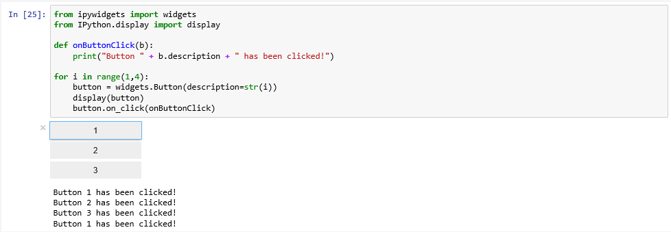
Note- the following might not apply to Notebooks in Pro, but it is good information to know if and when using the stand alone Jupyter Notebook session. Doing this outside of Pro’s Package Manager might corrupt your environment so be sur to perform this on a dedicated env clone.
If you get an error with this code "Failed to display Jupyter Widget of type Button" that means the widgets are probably not installed which we can potentially fix in our Anaconda prompt:
conda install -n base -c conda-forge widgetsnbextension conda install -n AC37 -c conda-forge ipywidgets
After installing the packages, exit your Jupyter notebook and restart it and try to re-run your code. It is possible you will receive the error again as the widget tries to run before the Javascript library that runs the widgets has opened. In that case try to select your code, wait a few more seconds and then click Run.
If you are still getting an error, it is likely that your packages did not install properly (or in a way that Jupyter/Anaconda could find them). The fix for this is to close Jupyter Notebook, return to Anaconda Navigator, click Environments (on the left), choose your environment and then search for "ipy", you may need to either change the "Installed" dropdown to "Not Installed" if they are missing or perhaps they should be updated (by clicking on the upward point arrow or the blue text).

It is easy to imagine how this example could be extended to provide some choices on how the next analysis step in a longer Data Science project should be performed. Similarly, a slider or text input field could be used to allow the notebook user to change the values of important input variables.
Lesson content developed by Jan Wallgrun and James O’Brien
Autocompletion, Restarting the Kernel, and other useful things
Let’s close this brief introduction to Jupyter with a few more things that are good to know when starting to write longer and more complex notebooks. Like normal development environments, Juypter has an autocomplete feature that helps with the code writing and can save a lot of typing: while editing code in a code cell, you can press the TAB key and Jupyter will either automatically complement the name or keyword you are writing or provide you with a dropdown list of choices that you can pick from. For instance, type in soup.ge and then press TAB and you get the list of options, as shown in Figure 3.13 including the get_text() function that we used in our code.

Another useful keyboard command to remember is SHIFT+TAB. When you place the cursor on a variable name or function call and press this key combination, a window will open up showing helpful information like the type of the variable and its current content or the parameters of the function as in Figure 3.14. This is of great help if you are unsure about the different parameters of a function, their order or names. Try out what you get when you use this key combination for different parts of the code in this notebook.

As in all programming, it may occasionally happen that something goes completely wrong and the execution of the code in a cell won’t terminate in the expected time or not at all. If that happens, the first thing to try is to use the “Interrupt Kernel” button located to the right of the “Execute cell” button. This should stop the execution of the current cell and you can then modify the code and try to run the cell again. However, sometimes even that won’t help because the kernel has become unresponsive. In that case, the only thing you can do is restart the kernel using the “Restart Kernel” button to the right of the “Interrupt Kernel” button. Unfortunately, that means that you will have to start the execution of the code in your notebook from the beginning because all imports and variable assignments will be lost after the restart.
Once you have finished your notebook, you may want to publish or share it. There are many options by wich to do so. In the File menu, there exists the “Download as…” option for obtaining versions of your notebook in different formats. The .ipynb format, as we mentioned, is the native format in which Jupyter saves the notebooks. If you make the .ipynb file available to someone who has access to Juypter, that person can open the notebook and run it or modify the content. The .py option allows for exporting content as a Python script, so that the code can be run outside of Jupyter. If you want a version of your notebook that others can read even without access to Jupyter, there are several options like exporting the notebook as HTML, as Latex, or as PDF. Some of these options require additional software tools to be installed on your computer and there are some limitations. For instance, if you export your notebook as HTML to add it to your personal web page, interactive widgets such as the interactive web map will not be included.
To close this section, we want to again refer to the links we provided at the beginning of this section if you want to keep reading about Jupyter and learn tricks that we weren't able to cover in this brief introduction.
Lesson content developed by Jan Wallgrun and James O’Brien
Practice Exercises
The goal of this exercise is to practice creating GUIs a little bit more. Your task is to implement a rudimentary calculator application for just addition and subtraction that should look like the image below:

The buttons 0… 9 are for entering the digits into the line input field at the top. The buttons + and - are for selecting the next mathematical operation and performing the previously selected one. The = button is for performing the previously selected operation and printing out the result, and the “Clear” button is for resetting everything and setting the content of the central line edit widget to 0. At the top of the calculator we have a combo box that will list all intermediate results and, on selection of one of the entries, will place that number in the line edit widget to realize a simple memory function.
Here is what you will have to do:
- Create the GUI for the calculator with QT Designer using the “Widget” template. This calculator app is very simple so we will use QWidget for the main window, not QMainWindow. Make sure you use intuitive object names for the child widgets you add to the form. (See Sections 2.6.2 and 2.7.2)
- Compile the .ui file created in QT Designer into a .py file (Sections 2.6.2 and 2.7.2).
- Set up a main script file for this project and put in the code to start the application and set up the main QWidget with the help of the .py file created in step 2 (Sections 2.6.1 and 2.7.3).
Hint 1: To produce the layout shown in the figure above, the horizontal and vertical size policies for the 10 digit buttons have been set to “Expanding” in QT Designer to make them fill up the available space in both dimensions. Furthermore, the font size for the line edit widget has been increased to 20 and the horizontal alignment has been set to “AlignRight”.
This is the main part we want you to practice with this exercise. You should now be able to run the program and have the GUI show up as in the image above but without anything happening when you click the buttons. If you want, you can continue and actually implement the functionality of the calculator yourself following the steps below, or just look at the solution code showing you how this can be done.
- Set up three global variables: intermediateResult for storing the most recent intermediate result (initialized to zero); lastOperation for storing the last mathematical operation picked (initialized to None); and numberEntered for keeping track of whether or not there have already been digits entered for a new number after the last time the +, -, = or Clear buttons have been pressed (initialized to False).
- Implement the event handler functions for the buttons 0 … 9 and connect them to the corresponding signals. When one of these buttons is pressed, the digit should either be appended to the text in the line edit widget or, if its content is “0” or numberEntered is still False, replace its content. Since what needs to happen here is the same for all the buttons, just using different numbers, it is highly recommended that you define an auxiliary function that takes the number as a parameter and is called from the different event handler functions for the buttons.
- Implement an auxiliary function that takes care of the evaluation of the previously picked operation when, e.g., the = button is clicked. If lastOperation contains an operation (so is not None), a new intermediate result needs to be calculated by applying this operation to the current intermediate result and the number in the line edit widget. The new result should appear in the line edit widget. If lastOperation is None, then intermediateResult needs to be set to the current text content of the line input widget. Create the event handler function for the = button and connect it to this auxiliary function.
- Implement and connect the event handler functions for the buttons + and - . These need to call the auxiliary function from the previous step and then set lastOperation to a string value representing the new operation that was just picked, either "+" or "-".
- Implement and connect the event handler for the “Clear” button. Clicking it means that the global variables need be re-initialized as in step 4 and the text content of the line edit widget needs to be set back to “0”.
- Implement the combo box functionality: whenever a calculation is performed by the auxiliary function from step 6, you now also need to add the result to the item list of the memory combo box. Furthermore, you need to implement and connect the event handler for when a different value from the combo box is picked and make this the new text content of the line edit field. The signal of the combo box you need to connect to for this is called “activated”.
Practice Exercise solution
The image below shows the hierarchy of widgets created in QT Designer and the names chosen. You can also download the .ui file and the compiled .py version here [119] and open the .ui file in QT Designer to compare it to your own version. Note that we are using a vertical layout as the main layout, a horizontal layout within that layout for the +, -, =, and Clear button, and a grid layout within the vertical layout for the digit buttons.

The following code can be used to set up the GUI and run the application but without yet implementing the actual calculator functionality. You can run the code and main window with the GUI you created will show up.
import sys from PyQt5.QtWidgets import QApplication, QWidget import calculator_gui # create application and gui app = QApplication(sys.argv) mainWindow = QWidget() # create an instance of QWidget for the main window ui = calculator_gui.Ui_Form() # create an instance of the GUI class from calculator_gui.py ui.setupUi(mainWindow) # create the GUI for the main window # run app mainWindow.show() sys.exit(app.exec_())
The main .py file for the full calculator can be downloaded here [120]. Function digitClicked(…) is the auxiliary function from step 5, called by the ten event handler functions digitPBClicked(…) defined later in the code. Function evaluateResult() is the auxiliary function from step 6. Function operatorClicked(…) is called from the two event handler functions plusPBClicked() and minusPBClicked(), just with different strings representing the mathematical operation. There are plenty of comments in the code, so it should be possible to follow along and understand what is happening rather easily.
Lesson 4 Assignment
In this homework assignment, we want you to create a script tool or Jupyter Notebook (using Pro’s base environment).
You can use a previous lesson assignment’s script, or you can create a new one that is pertinent to your work or interest. If you choose to do the later, include a sample dataset that can be used to test your script tool or Jupyter Notebook and include in your write-up the necessary steps taken for the script tool or Notebook to work.
Write-up
Produce a 400-word write-up on how the assignment went for you; reflect on and briefly discuss the issues and challenges you encountered and what you learned from the assignment.
Deliverable
Submit a single .zip file to the corresponding drop box on Canvas; the zip file should contain:
- Your script file
- Your 400-word write-up