Lesson 4: GUI Development
We made it to the final week of this course! That deserves congratulations and a pat on the back! In this lesson, we will look at creating software applications to give our scripts and code a means to be used outside of the IDE or command line. This lesson covers ESRI’s script tool, introduces the ArcGIS for .Net SDK (which is beyond the scope of this course and would take another 8 weeks to dive into), Python's GUI (Graphic User Interface) development PyQT, Open source QGIS, and lastly Jupyter Notebooks.
Special note- The QGIS and OSGEO environment can be temperamental and while QGIS is topic covered by this lesson, setting it up can often take a week or longer. I suggest reading over the PyQt / QGIS content and just be aware of its syntax and implementation. You can also explore the full topic here [1] and get a complete context for QGIS. I would encourage you to try it if you have the time.
All good things must come to an end, so let's get started!
Overview and Checklist
In this final lesson we will look at creating software applications to give our scripts a means to be used outside of the IDE or command line. This lesson covers ESRI’s script tool, introduces the ArcGIS for .Net SDK (which is beyond the scope of this course and would take another 8 weeks to dive into), Pythons GUI (Graphic User Interface) development PyQT, Open source QGIS, and Jupyter Notebook
Detailed content for this lesson was drastically reduced to keep it manageable and I would encourage you to reference the full 489 course if you are interested in any of the technologies covered. We will wrap up the course with the final assignment that involves you converted one of your previous assignment scripts to a script tool or Jupyter Notebook. The script you choose to convert will be up to you and you will indicate which one you choose in the Lesson 4 assignment discussion. Feel free to post any questions you may have to the forum and please help each other out. The more exposure you get to code, the better you will be at coding.
With that, the end is in sight and if you have any questions that were not covered so far, please feel free to ask!
Learning Outcomes
By the end of this lesson, you should be able to:
- Operations on data lists
- Use regex to perform data extraction.
- Identify the main python packages used for spatial data science.
- Perform data manipulation using Pandas.
Lesson Roadmap
| Step | Activity | Access/Directions |
|---|---|---|
| 1 | Engage with Lesson 4 Content | Begin with 4.1 Making a script tool |
| 2 | Programming Assignment and Reflection | Submit your code for the programming assignment and 400 words write-up with reflections |
| 3 | Quiz 4 | Complete the Lesson 4 Quiz |
| 4 | Questions/Comments | Remember to visit Canvas to post/answer any questions or comments pertaining to Lesson 4 |
Downloads
The following is a list of datasets that you will be prompted to download through the course of the lesson. They are divided into two sections: Datasets that you will need for the assignments and Datasets used for the content and examples in the lesson.
Required:
- None for lesson!
Suggested:
- TM_WORLD_BORDERS [2]
Assignment
In this homework assignment, we want you to create a script tool or Jupyter Notebook (using Pro’s base environment).
You can use a previous lesson assignment’s script, or you can create a new one that is pertinent to your work or interest. If you choose to do the later, include a sample dataset that can be used to test your script tool or Jupyter Notebook and include in your write-up the necessary steps taken for the script tool or Notebook to work.
Write-up
Produce a 400-word write-up on how the assignment went for you; reflect on and briefly discuss the issues and challenges you encountered and what you learned from the assignment.
Deliverable
Submit a single .zip file to the corresponding drop box on Canvas; the zip file should contain:
- Your script file
- Your 400-word write-up
Questions?
If you have any questions, please send a message through Canvas. We will check daily to respond. If your question is one that is relevant to the entire class, we may respond to the entire class rather than individually.
Making A Script Tool
User input variables that you retrieve through GetParameterAsText() make your script very easy to convert into a tool in ArcGIS. A few people know how to alter Python code, a few more can run a Python script and supply user input variables, but almost all ArcGIS users know how to run a tool. To finish off this lesson, we’ll take the previous script and make it into a tool that can easily be run in ArcGIS.
Before you begin this exercise, I strongly recommend that you scan the ArcGIS help topic Adding a script tool [3]. You likely will not understand all the parts of this topic yet, but it will give you some familiarity with script tools that will be helpful during the exercise.
Sample code for this section is below:
# This script runs the Buffer tool. The user supplies the input
#  and output paths, and the buffer distance.

import arcpy
arcpy.env.overwriteOutput = True

try:
     # Get the input parameters for the Buffer tool
     inPath = arcpy.GetParameterAsText(0)
     outPath = arcpy.GetParameterAsText(1)
     bufferDistance = arcpy.GetParameterAsText(2)

     # Run the Buffer tool
     arcpy.Buffer_analysis(inPath, outPath, bufferDistance)

     # Report a success message
     arcpy.AddMessage("All done!")

except Exception as ex:
     # Report an error messages
     arcpy.AddError(f"Could not complete the buffer {ex}")

     # Report any error messages that the Buffer tool might have generated
     arcpy.AddMessage(arcpy.GetMessages())
Follow these steps to make a script tool:
- Copy the code above into a new PyScripter script and save it as buffer_user_input.py.
- Open an ArcGIS Pro project and display the Catalog window.
- Expand the nodes Toolboxes > Default.tbx or .atbx. Your toolbox may be named differently, such as using the name of the project. For simplicity, we will refer to it as 'Default' for this lesson.
- Right-click on the Default.tbx and click New > Script.
- Fill in the Name and Label properties for your Script tool as shown below, depending on your version of ArcGIS Pro: The first image below shows the interface and the information you have to enter under General in this and the next step if you have a version earlier than version 2.9. The other two images show the interface and information that needs to be entered in this and the next step under General and under Execution if you have version 2.9 (or higher).
 Figure 1.10a Entering information for your script tool if you have a version < 2.9.
 Figure 1.10b Entering information for your script tool if you have a version ≥ 2.9: General tab.
 Figure 1.10c Entering information for your script tool if you have a version ≥ 2.9: Execution tab.
 - For version <2.9, click the folder icon for Script File on the General tab and browse to your buffer_user_input.py file. For version 2.9 (or higher), do the same on the Execution tab; the code from the script file will be shown in the window below.
- All versions: On the left side of the dialog, click on Parameters. You will now enter the parameters needed for this tool to do its job, namely inPath, outPath, and bufferMiles. You will specify the parameters in the same order, except you can give the parameters names that are easier to understand.
- Working in the first row of the table, enter Input Feature Class in the Label column, then Tab out of that cell. Note that the Name column is automatically filled in with the same text, except that the spaces are replaced by spaces.
- Next, click in the Data Type column and choose Feature Class from the subsequent dialog. Here is one of the huge advantages of making a script tool. Instead of accepting any string as input (which could contain an error), your tool will now enforce the requirement that a feature class be used as input. ArcGIS will help you by confirming that the value entered is a path to a valid feature class. It will even supply the users of your tool with a browse button, so they can browse to the feature class.
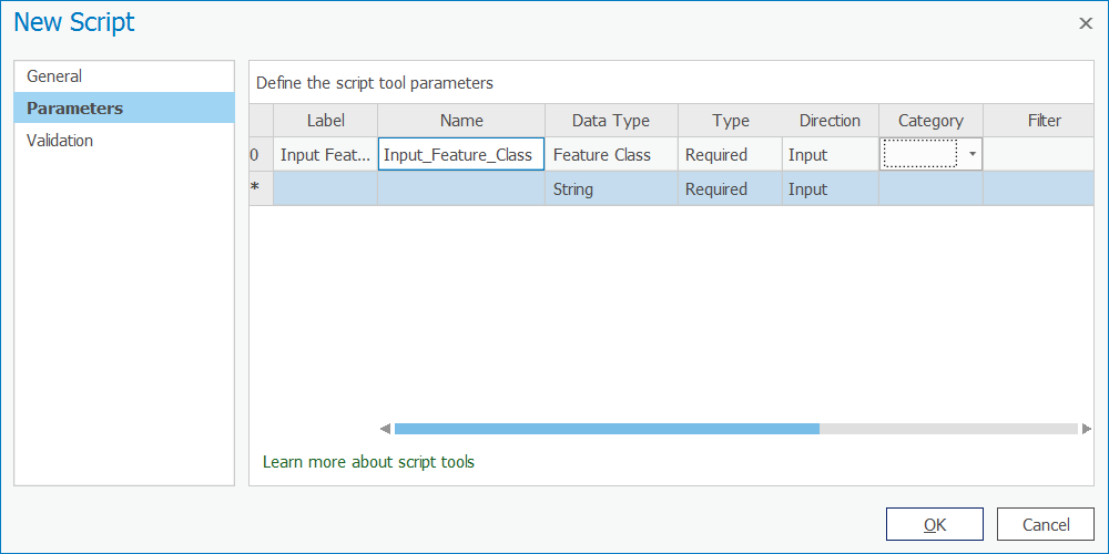 Figure 1.11 Choosing "Feature Class."
 - Just as you did in the previous steps, add a second parameter labeled Output Feature Class. The data type should again be Feature Class.
- For the Output Feature Class parameter, change the Direction property to Output.
- Add a third parameter named Buffer Distance. Choose Linear Unit as the data type. This data type will allow the user of the tool to select both the distance value and the units (for example, miles, kilometers, etc.).
- Set the Buffer Distance parameter's Default property to 5 Miles. (You may need to scroll to the right to see the Default column.) Your dialog should look like what you see below:
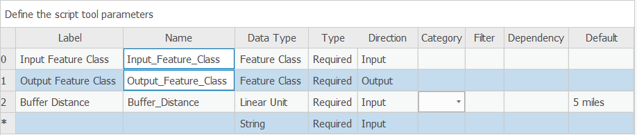 Figure 1.12 Setting the Default property to "5 Miles."
 - Click OK to finish creation of the new script tool and open it by double-clicking it.
- Try out your tool by buffering any feature class on your computer. Notice that once you supply the input feature class, an output feature class path is suggested for you. This is because you specifically set Output Feature Class as an output parameter. Also, when the tool is complete, examine the Details box (visible if you hover your mouse over the tool's "Completed successfully" message) for the custom message "All done!" that you added in your code.
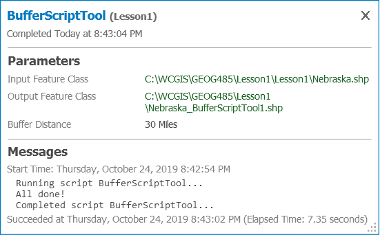 Figure 1.13 The tool is complete.
This is a very simple example, and obviously, you could just run the out-of-the-box Buffer tool with similar results. Normally, when you create a script tool, it will be backed with a script that runs a combination of tools and applies some logic that makes those tools uniquely useful.
There’s another benefit to this example, though. Notice the simplicity of our script tool dialog compared to the main Buffer tool:
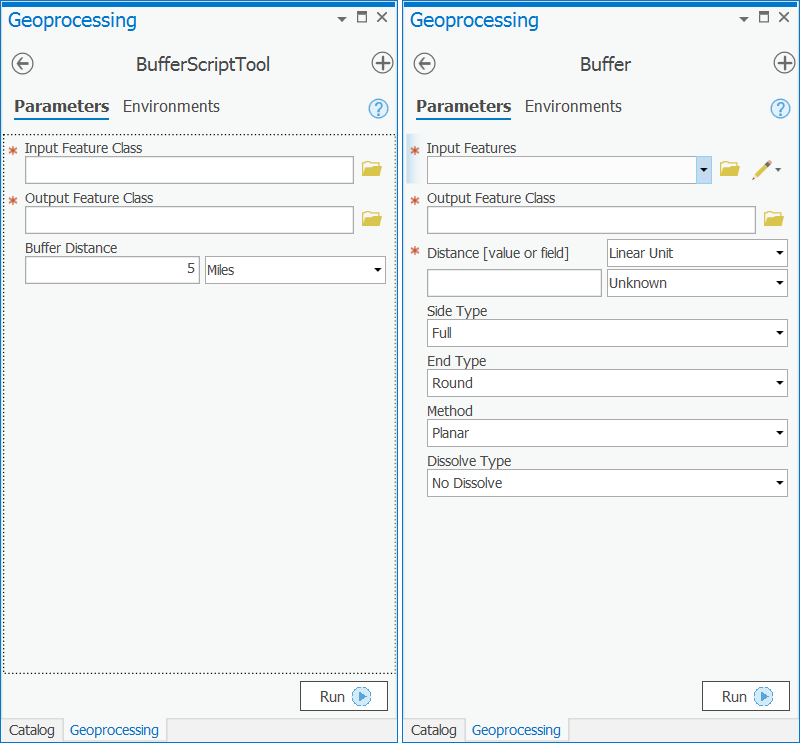
At some point, you may need to design a set of tools for beginning GIS users where only the most necessary parameters are exposed. You may also do this to enforce quality control if you know that some of the parameters must always be set to certain defaults, and you want to avoid the scenario where a beginning user (or a rogue user) might change the required values. A simple script tool is effective for simplifying the tool dialog in this way.
Lesson content developed by Jim Detwiler, Jan Wallgrun and James O’Brien
Adding Tool Validation Code
Now let’s expand on the user friendliness of the tool by using the validator methods to ensure that our cutoff value falls within the minimum and maximum values of our raster (otherwise performing the analysis is a waste of resources).
The purpose of the validation process is to allow us to have some customizable behavior depending on what values we have in our tool parameters. For example, we might want to make sure a value is within a range as in this case (although we could do that within our code as well), or we might want to offer a user different options if they provide a point feature class instead of a polygon feature class, or different options if they select a different type of field (e.g. a string vs. a numeric type).
The Esri help for Tool Validation(link is external) [4] gives a longer list of uses and also explains the difference between internal validation (what Desktop & Pro do for us already) and the validation that we are going to do here which works in concert with that internal validation.
You will notice in the help that Esri specifically tells us not to do what I’m doing in this example – running geoprocessing tools. The reason for this is they generally take a long time to run. In this case, however, we’re using a very simple tool which gets the minimum & maximum raster values and therefore executes very quickly. We wouldn’t want to run an intersection or a buffer operation for example in the ToolValidator, but for something very small and fast such as this value checking, I would argue that it’s ok to break Esri’s rule. You will probably also note that Esri hints that it’s ok to do this by using Describe to get the properties of a feature class and we’re not really doing anything different except we’re getting the properties of a raster.
So how do we do it? Go back to your tool (either in the Toolbox for your Project, Results, or the Recent Tools section of the Geoprocessing sidebar), right click and choose Properties and then Validation.
You will notice that we have a pre-written, Esri-provided class definition here. We will talk about how class definitions look in Python in Lesson 4 but the comments in this code should give you an idea of what the different parts are for. We’ll populate this template with the lines of code that we need. For now, it is sufficient to understand that different methods (initializeParameters(), updateParameters(), etc.) are defined that will be called by the script tool dialog to perform the operations described in the documentation strings following each line starting with def.
Take the code below and use it to overwrite what is in your ToolValidator:
import arcpy
class ToolValidator(object):
"""Class for validating a tool's parameter values and controlling
the behavior of the tool's dialog."""
def __init__(self):
"""Setup arcpy and the list of tool parameters."""
self.params = arcpy.GetParameterInfo()
def initializeParameters(self):
"""Refine the properties of a tool's parameters. This method is
called when the tool is opened."""
def updateParameters(self):
"""Modify the values and properties of parameters before internal
validation is performed. This method is called whenever a parameter
has been changed."""
def updateMessages(self):
"""Modify the messages created by internal validation for each tool
parameter. This method is called after internal validation."""
## Remove any existing messages
self.params[1].clearMessage()
if self.params[1].value is not None:
## Get the raster path/name from the first [0] parameter as text
inRaster1 = self.params[0].valueAsText
## calculate the minimum value of the raster and store in a variable
elevMINResult = arcpy.GetRasterProperties_management(inRaster1, "MINIMUM")
## calculate the maximum value of the raster and store in a variable
elevMAXResult = arcpy.GetRasterProperties_management(inRaster1, "MAXIMUM")
## convert those values to floating points
elevMin = float(elevMINResult.getOutput(0))
elevMax = float(elevMAXResult.getOutput(0))
## calculate a new cutoff value if the original wasn't suitable but only if the user hasn't specified a value.
if self.params[1].value < elevMin or self.params[1].value > elevMax:
cutoffValue = elevMin + ((elevMax-elevMin)/100*90)
self.params[1].value = cutoffValue
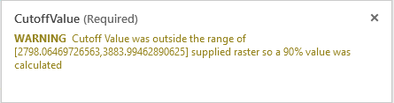
self.params[1].setWarningMessage("Cutoff Value was outside the range of ["+str(elevMin)+","+str(elevMax)+"] supplied raster so a 90% value was calculated")
Our logic here is to take the raster supplied by the user and determine the min and max values so that we can evaluate whether the cutoff value supplied by the user falls within that range. If that is not the case, we're going to do a simple mathematical calculation to find the value 90% of the way between the min and max values and suggest that as a default to the user (by putting it into the parameter). We’ll also display a warning message to the user telling them that the value has been adjusted and why their original value doesn’t work.
As you look over the code, you’ll see that all of the work is being done in the bottom function updateMessages(). This function is called after the updateParameters() and the internal arcpy validation code have been executed. It is mainly intended for modifying the warning or error messages produced by the internal validation code. The reason why we are putting all our validation code here is because we want to produce the warning message and there is no entirely simple way to do this if we already perform the validation and potentially automatic adjustment of the cutoff value in updateParameters() instead. Here is what happens in the updateMessages() function:
We start by cleaning up any previous messages self.params[1].clearMessages() (line 24). Then we check if the user has entered a value into the cutoffValue parameter (self.params[1]) on line 26. If they haven't, we don’t do anything (for efficiency). If the user has entered a value (i.e., the value is not None) then we get the raster name from the first parameter (self.params[0]) and we extract it as text (because we want the content to use as a path) on line 28. Then we’ll call the arcpy GetRasterProperties function twice, once to get the min value (line 30) and again to get the max value (on line 32) of the raster. We’ll then convert those values to floating point numbers (lines 34 & 35).
Once we’ve done that, we do a little bit of checking to see if the value the user supplied is within the range of the raster. If it is not, then we will do some simple math to calculate a value that falls 90% of the way into the range and then update the parameter (self.params[1].value) with the number we calculated (line 40 and 41). Finally, in line 42, we produce the warning message informing the users of the automatic value adjustment.
Now let’s test our Validator. Click OK and return to your script in the Toolbox, Results or Geoprocessing window. Run the script again. Insert the name of the input raster again. If you didn’t make any mistakes entering the code there won’t be a red X by the Input Raster. If you did make a mistake, an error message will be displayed there, showing you the usual arcpy / geoprocessing error message and the line of code that the error is occurring on. If you have to do any debugging, exit the script, return to the Toolbox, right click the script and go back to the Tool Validator and correct the error. Repeat as many times as necessary.
If there were no errors, we should test out our validation by putting a value into our Cutoff Value parameter that we know to be outside the range of our data. If you choose a value < 2798 or > 3884, you should see a yellow warning triangle appear that displays our error message, and you will also note that the value in Cutoff Value has been updated to our 90% value.
We can change the value to one we know works within the range (e.g. 3500), and now the tool should run.
Lesson content developed by Jan Wallgrun and James O’Brien
ArcGIS Pro Add-in Introduction
ESRI provides the ability to extend and customize the Pro application through the ArcGIS Pro SDK for .Net [5]. The SDK provides access to much of the Pro application framework to include creating custom ribbon menu’s and buttons, branded configurations, custom geoprocessing ‘add-ins’.
Since each ArcGIS Pro project’s folders, toolboxes, databases, etc.,. is compartmentalized to the project, the user needs to add the custom toolbox with the script tools from the favorites or set the toolbox to be added to new projects. This can get confusing for some users. One benefit of using the SDK and creating Add-ins for the custom geoprocessing tools is the way they are deployed to the user. The add-in is deployed through the addinx through the addin manager. It can be hosted on a network shared folder, installed locally, or hosted for download on the Organizations Portal and is loaded for every project. Instead of running script tool from a toolbox, the tool is loaded from clicking the button on the Ribbon Menu.
Another difference between the add-in and script tool that may be useful for some geoprocessing workflows is the ability to create dynamic interactivity into the add-in and work with features in the mapview. Script tools are linear and require the user input and settings before it is started. You can do some limited interactivity such as extent, selection, and loaded layers but Add-ins can provide the ability to work through the process dynamically. An example might be creating a tool that assists non-gis users the ability to edit attributes through a UI (User Interface) and code tailored to that dataset. You can perform CRUD operations on a table of data while providing the user with informational prompt messages that take user input.
To create the add-in, knowledge of the C# language and WPF (Windows Presentation Format) architecture is needed and is unfortunately beyond the scope of this course. Esri provides instructor led training courses as well as a lot of complete SDK samples (as visual studio projects), code snippets, and tutorials in their SDK documentation and Github repository.
PyQt (overview)
While it’s good and useful to understand how to write Python code to create a GUI directly, it’s obviously a very laborious and time consuming approach that requires writing a lot of code. So together with the advent of early GUI frameworks, people also started to look into more visual approaches in which the GUI of a new software application is clicked and dragged together from predefined building blocks. The typical approach is that first the GUI is created within the graphical GUI building tool and then the tool translates the graphical design into code of the respective programming language that is then included into the main code of the new software application.
Note that this too could be an 8 week course as well and due to time contraints, this is provided as an overview. If you are interested in exploring it more, please view the full topic in the full 10-week course content [7].
Creating GUIs with QT Designer 2.6.2
The GUI building tool for QT that we are going to use in this lesson is called QT Designer. QT Designer is included in the PyQT5 Python package and can be installed through ArcGIS Pro Python Package manager. The tool itself is platform and programming language independent. Instead of producing code from a particular programming language, it creates a .ui file with an xml description of the QT-based GUI. This .ui file can then be translated into Python code with the pyuic5 GUI compiler tool that also comes with PyQT5. There is also support for directly reading the .ui file from Python code in PyQT5 and then generating the GUI from its content, but we here demonstrate the approach of creating the Python code with pyui5 because it is faster and allows us to see and inspect the Python code for our application. In the following, we will take a quick look at how the QT Designer works.
You can install PyQt5 from the ArcGIS Pro package manager. The QT Designer executable will be in your ArcGIS Pro Python environment folder, either under "C:\Users\<username>\AppData\Local\ESRI\conda\envs\arcgispro-py3-clone\Library\bin\designer.exe" or under “C:\Program Files\ArcGIS\Pro\bin\Python\envs\arcgispro-py3\Library\bin\designer.exe”. It might be good idea to create a shortcut to this .exe file on your desktop for the duration of the course, allowing you to directly start the application. After starting, QT Designer will greet you as shown in the figure below:

QT Designer allows for creating so-called “forms” which can be the GUI for a dialog box, a main window, or just a simple QWidget. Each form is saved as a single .ui file. To create a new form, you pick one of the templates listed in the “New Form” dialog. Go ahead and double-click the “Main Window” template. As a result, you will now see an empty main window form in the central area of the QT Designer window.

Let’s quickly go through the main windows of QT Designer. On the left side, you see the “Widget Box” pane that lists all the widgets available including layout widgets and spacers. Adding a widget to the current form can be done by simply dragging the widget from the pane and dropping it somewhere on the form. Go ahead and place a few different widgets like push buttons, labels, and line edits somewhere on the main window form. When you do a right-click in an empty part of the central area of the main window form, you can pick “Lay out” in the context menu that pops up to set the layout that should be used to arrange the child widgets. Do this and pick “Lay out horizontally” which should result in all the widgets you added being arranged in a single row. See what happens if you instead change to a grid or vertical layout. You can change the layout of any widget that contains other widgets in this way.
On the right side of QT Designer, there are three different panes. The one at the top called “Object Inspector” shows you the hierarchy of all the widgets of the current form. This currently should show you that you have a QMainWindow widget with a QWidget for its central area, which in turn has several child widgets, namely the widgets you added to it. You can pretty much perform the same set of operations that are available when interacting with a widget in the form (like changing its layout) with the corresponding entry in the “Object Inspector” hierarchy. You can also drag and drop widgets onto entries in the hierarchy to add new child widgets to these entries, which can sometimes be easier than dropping them on widgets in the form, e.g., when the parent widget is rather small.
The “Object” column lists the object name for each widget in the hierarchy. This name is important because when turning a GUI form into Python code, the object name will become the name of the variable containing that widget. So if you need to access the widget from your main code, you need to know that name and it’s a good idea to give these widgets intuitive names. To change the object name to something that is easier to recognize and remember, you can double-click the name to edit it, or you can use “Change objectName” from the context menu when you right-click on the entry in the hierarchy or the widget itself.
Below the “Object Inspector” window is the “Property Editor”. This shows you all the properties of the currently selected widget and allows you to change them. The yellow area lists properties that all widgets have, while the green and blue areas below it (you may have to scroll down to see these) list special properties of that widget class. For instance, if you select a push button you added to your main window form, you will find a property called “text” in the green area. This property specifies the text that will be displayed on the button. Click on the “Value” column for that property, enter “Push me”, and see how the text displayed on the button in the main window form changes accordingly. Some properties can also be changed by double-clicking the widget in the form. For instance, you can also change the text property of a push button or label by double-clicking it.
If you double-click where it says “Type Here” at the top, you can add a menu to the menu bar of the main window. Give this a try and call the menu “File”.

The last pane on the right side has three tabs below it. “Resource browser” allows for managing additional resources, like files containing icons to be used as part of the GUI. “Action editor” allows for creating actions for your GUI. Remember that actions are for things that can be initiated via different GUI elements. If you click the “New” button at the top, a dialog for creating a new action opens up. You can just type in “test” for the “Text” property and then press “OK”. The new action will now appear as actionTest in the list of actions. You can drag it and drop it on the File menu you created to make this action an entry in that menu.

Finally, the “Signal/Slot Editor” tab allows for connecting signals of the widgets and actions created to slots of other widgets. We will mainly connect signals with event handler functions in our own Python code rather than in QT Designer, but if some widgets’ signals should be directly connected to slots of other widgets this can already be done here.
You now know the main components of QT Designer and a bit about how to place and arrange widgets in a form. We cannot teach QT Designer in detail here but we will show you an example of creating a larger GUI in QT Designer as part of the following first walkthrough of this lesson. If you want to learn more, there exist quite a few videos explaining different aspects of how to use QT Designer on the web. For now, here is a short video (12:21min) that we recommend checking out to see a few more basic examples of the interactions we briefly described above before moving on to the walkthrough.
Video: Qt Designer - PyQt with Python GUI Programming tutorial [8] by sentdex [9]
Once you have created the form(s) for the GUI of your program and saved them as .ui file(s), you can translate them into Python code with the help of the pyuic5 tool, e.g. by running a command like the following from the command line using the tool directly with Python :
"C:\Users\<username>\AppData\Local\ESRI\conda\envs\arcgispro-py3-clone\python.exe" –m PyQt5.uic.pyuic mainwindow.ui –o mainwindow.py
or
"C:\Program Files\ArcGIS\Pro\bin\Python\envs\arcgispro-py3\python.exe" –m PyQt5.uic.pyuic mainwindow.ui –o mainwindow.py
depending on where your default Python environment is located (don't forget to replace <username> with your actual user name in the first version and if you get an error with this command try typing it in, not copying/pasting). mainwindow.ui, here, is the name of the file produced with QT Designer, and what follows the -o is the name of the output file that should be produced with the Python version of the GUI. If you want, you can do this for your own .ui file now and have a quick look at the produced .py file and see whether or not you understand some of the things happening in it. We will demonstrate how to use the produced .py file to create the GUI from your Python code as part of the walkthrough in the next section.
Lesson content developed by Jan Wallgrun and James O’Brien
The QGIS Scripting Interface and Python API 4.5
Interacting with Layers Open in QGIS 4.5.1
Let us start this introduction by writing some code directly in the QGIS Python console and talking about how you can access the layers currently open in QGIS and add new layers to the currently open project. If you don’t have QGIS running at the moment, please start it up and open the Python console from the Plugins menu in the main menu bar.
When you open the Python console in QGIS, the Python qgis package and its submodules are automatically imported as well as other relevant modules including the main PyQt5 modules. In addition, a variable called iface is set up to provide an object of the class QgisInterface1 [10] to interact with the running QGIS environment. The code below shows how you can use that object to retrieve a list of the layers in the currently open map project and the currently active layer. Before you type in and run the code in the console, please add a few layers to an empty project including the TM_WORLD_BORDERS-0.3.shp shapefile (download here) [11]. We will recreate some of the steps from that section with QGIS here so that you also get a bit of a comparison between the two APIs (Application Programming Interfaces). The currently active layer is the one selected in the Layers window; please select the world borders layer by clicking on it before you execute the code.
layers = iface.mapCanvas().layers()
for layer in layers:
    print(layer)
    print(layer.name())
    print(layer.id())
    print('------')
# If you copy/paste the code - run the part above
# before you run the part below
# otherwise you'll get a syntax error.
activeLayer = iface.activeLayer()
print('active layer: ' + activeLayer.name())
Output (numbers will vary): ...TM_WORLD_BORDERS-0.3 TM_WORLD_BORDERS_0_3_2e5a7cd5_591a_4d45_a4aa_cbba2e639e75 ------ ... active layer: TM_WORLD_BORDERS-0.3
The layers() method of the QgsMapCanvas [12] object we get from calling iface.mapCanvas() returns the currently open layers as a list of objects of the different subclasses of QgsMapLayer [13]. Invoking the name() method of these layer objects gives us the name under which the layer is listed in the Layers window. layer.id() gives us the ID that QGIS has assigned to the layer which in contrast to the name is unique. The iface.activeLayer() method gives us the currently selected layer.
The type() function of a layer can be used to test the type of the layer:
if activeLayer.type() == QgsMapLayer.VectorLayer:
    print('This is a vector layer!')
Depending on the type of the layer, there are other methods that we can call to get more information about the layer. For instance, for a vector layer [14] we can use wkbType() to get the geometry type of the layer:
if activeLayer.type() == QgsMapLayer.VectorLayer:
    if activeLayer.wkbType() == QgsWkbTypes.MultiPolygon:
        print('This layer contains multi-polygons!')
The output you get from the previous command should confirm that the active world borders layer contains multi-polygons, meaning features that can have multiple polygonal parts.
QGIS defines a function dir(…) that can be used to list the methods that can be invoked for a given object. Try out the following two applications of this function:
dir(iface)
dir(activeLayer)
To add or remove a layer, we need to work with the QgsProject [15] object for the project currently open in QGIS. We retrieve it like this:
currentProject = QgsProject.instance()
print(currentProject.fileName())
The output from the print statement in the second row will probably be the empty string unless you have saved the project. Feel free to do so and rerun the line and you should get the actual file name.
Here is how we can remove the active layer (or any other layer object) from the layer registry of the project (you may have to resize/refresh the map canvas afterwards for the layer to disappear there):
currentProject.removeMapLayer(activeLayer.id())
The following command shows how we can add the world borders shapefile again (or any other feature class we have on disk). Make sure you adapt the path based on where you have the shapefile stored. We first have to create the vector layer object providing the file name and optionally the name to be used for the layer. Then we add that layer object to the project via the addMapLayer(…) method:
layer = QgsVectorLayer(r'C:\489\TM_WORLD_BORDERS-0.3.shp', 'World borders')
currentProject.addMapLayer(layer)
Lastly, here is an example that shows you how you can change the symbology of a layer from your code:
renderer = QgsGraduatedSymbolRenderer()
renderer.setClassAttribute('POP2005')
layer.setRenderer(renderer)
layer.renderer().updateClasses(layer, QgsGraduatedSymbolRenderer.Jenks, 5)
layer.renderer().updateColorRamp(QgsGradientColorRamp(Qt.white, Qt.red))
iface.layerTreeView().refreshLayerSymbology(layer.id())
iface.mapCanvas().refreshAllLayers()
Here we create an object of the QgsGraduatedSymbolRenderer class that we want to use to draw the country polygons from our layer using a graduated color approach based on the population attribute ‘POP2005’. The name of the field to use is set via the renderer’s setClassAttribute() method in line 2. Then we make the renderer object the renderer for our world borders layer in line 3. In the next two lines, we tell the renderer (now accessed via the layer method renderer()) to use a Jenks Natural Breaks classification with 5 classes and a gradient color ramp that interpolates between the colors white and red. Please note that the colors used as parameters here are predefined instances of the Qt5 class QColor. Changing the symbology does not automatically refresh the map canvas or layer list. Therefore, in the last two lines, we explicitly tell the running QGIS environment to refresh the symbology of the world borders layer in the Layers tree view (line 6) and to refresh the map canvas (line 7). The result should look similar to the figure below (with all other layers removed).

[1] The qgis Python module is a wrapper around the underlying C++ library. The documentation pages linked in this section are those of the C++ version but the names of classes and available functions and methods are the same.
Lesson content developed by Jan Wallgrun and James O’Brien
Accessing the Features of a Layer
Let’s keep working with the world borders layer open in QGIS for a bit, looking at how we can access the individual features in a layer and select features by attribute. The following piece of code shows you how we can loop through all the features with the help of the layer’s getFeatures() method:
for feature in layer.getFeatures():
    print(feature)
    print(feature.id())
    print(feature['NAME'])
    print('-----')
Output:
<qgis._core.QgsFeature object at 0x...>
0
Antigua and Barbuda
-----
<qgis._core.QgsFeature object at 0x...>
1
Algeria
-----
<qgis._core.QgsFeature object at 0x...>
2
Azerbaijan
-----
<qgis._core.QgsFeature object at 0x...>
3
Albania
-----
...
Features are represented as objects of the class QgsFeature(link is external) [16] in QGIS. So, for each iteration of the for-loop in the previous code example, variable feature will contain a QgsFeature object. Features are numbered with a unique ID that you can obtain by calling the method id() as we are doing in this example. Attributes like the NAME attribute of the world borders polygons can be accessed using the attribute name as the key as also demonstrated above.
Like in most GIS software, a layer can have an active selection. When the layer is open in QGIS, the selected features are highlighted. The layer method selectAll() allows for selecting all features in a layer and removeSelection() can be used to clear the selection. Give this a try by running the following two commands in the QGIS Python console and watch how all countries become selected and then deselected again.
layer.selectAll()
layer.removeSelection()
The method selectByExpression() allows for selecting features based on their properties with a SQL query string that has the same format as in ArcGIS. Use the following command to select all features from the layer that have a value larger than 300,000 in the AREA column of the attribute table. The result should look as in the figure below.
layer.selectByExpression('"AREA" > 300000')

While there can only be one active selection for a layer, you can create as many subgroups of features from a layer as you want by calling getFeatures(…) with a parameter that is an object of the class QgsFeatureRequest [17] and that has been given a filter expression via its setFilterExpression(…) method. The filter expression can be again an SQL query string. The following code creates a subgroup that will only contain the polygon for Canada. When you run it, this will not change the active selection that you see for that layer in QGIS but variable selectionName now provides access to the subgroup with just that one polygon. We get that first (and only) polygon by calling the __next__() method of selectionName and then print out some information about this particular polygon feature.
selectionName = layer.getFeatures(QgsFeatureRequest().setFilterExpression('"NAME" = \'Canada\''))
feature = selectionName.__next__()
print(feature['NAME'] + "-" + str(feature.id()))
print(feature.geometry())
print(feature.geometry().asWkt())
Output:
Canada – 23
<qgis._core.QgsGeometry object at 0x...>
MultiPolygon (((-65.61361699999997654 43.42027300000000878,...)))
The first print statement in this example works in the same way as you have seen before to get the name attribute and id of the feature. The method geometry() gives us the geometric object for this feature as an instance of the QgsGeometry class [18] and calling the method asWkt() gives us a WKT string representation of the multi-polygon geometry. You can also use a for-loop to iterate through the features in a subgroup created in this way. The method rewind() can be used to reset the iterator to the beginning so that when you call __next__() again, it will again give you the first feature from the subgroup.
When you have the geometry object and know what type of geometry it is, you can use the methods asPoint(), asPolygon(), asPolyline(), asMultiPolygon(), etc. to get the geometry as a Python data structure, e.g. in the case of multi-polygons as a list of lists of lists with each inner list containing tuples of the point coordinates for one polygonal component.
print(feature.geometry().asMultiPolygon())
[[[(-65.6136, 43.4203), (-65.6197,43.4181), … ]]]
Here is another example to demonstrate that we can work with several different subgroups of features at the same time. This time we request all features from the layer that have a POP2005 value larger than 50,000,000.
selectionPopulation = layer.getFeatures(QgsFeatureRequest().setFilterExpression('"POP2005" > 50000000'))
If we ever want to use a subgroup like this to create the active selection for the layer from it, we can use the layer method selectByIds(…) for this. The method requires a list of feature IDs and will then change the active selection to these features. In the following example, we use a simple list comprehension to create the ID list from the subgroup in our variable selectionPopulation:
layer.selectByIds([f.id() for f in selectionPopulation])
When running this command you should notice that the selection of the features in QGIS changes to look like in the figure below.

Let’s save the currently selected features as a new file. We use the GeoPackage format (GPKG) for this, which is more modern than the shapefile format, but you can easily change the command below to produce a shapefile instead; simply change the file extension to “.shp” and replace “GPKG” with “ESRI Shapefile”. The function we will use for writing the layer to disk is called writeAsVectorFormat(…) and it is defined in the class QgsVectorFileWriter [19]. Please note that this function has been declared "deprecated", meaning it may be removed in future versions and it is recommended that you do not use it anymore. In versions up to QGIS 3.16 (the current LTR version that most likely you are using right now), you are supposed to use writeAsVectorFormatV2(...) instead; however, there have been issues reported with that function and it is already replaced by writeAsVectorFormatV3(...) in versions >3.16 of QGIS. Therefore, we have decided to stick with writeAsVectorFormat(…) while things are still in flux. The parameters we give to writeAsVectorFormat(…) are the layer we want to save, the name of the output file, the character encoding to use, the spatial reference to use (we simply use the one that our layer is in), the format (“GPKG”), and True for signaling that only the selected features should be saved in the new data set. Adapt the path for the output file as you see fit and then run the command:
QgsVectorFileWriter.writeAsVectorFormat(layer, r'C:\489\highPopulationCountries.gpkg', 'utf-8', layer.crs(),'GPKG', True)
If you add the new file produced by this command to your QGIS project, it should only contain the polygons for the countries we selected based on their population values.
For changing the attribute values of a feature, we need to work with the “data provider” object of the layer. We can access it via the layer’s dataProvider() method:
dataProvider = layer.dataProvider()
Let’s say we want to change the POP2005 value for Canada to 1 (don’t ask what happened!). For this, we also need the index of the POP2005 column which we can get by calling the data provider’s fieldNameIndex() method:
populationColumnIndex = dataProvider.fieldNameIndex('POP2005')
To change the attribute value we call the method changeAttributeValues(…) of the data provider object providing a dictionary as parameter that maps feature IDs to dictionaries which in turn map column indices to new values. The inner dictionary that maps column indices to values is defined in a separate variable newValueDictionary.
newValueDictionary = { populationColumnIndex : 1 }
dataProvider.changeAttributeValues( { feature.id(): newValueDictionary } )
In this simple example, the outer dictionary contains only a single key-value pair with the ID of the feature for Canada as key and another dictionary as value. The inner dictionary also only contains a single key-value pair consisting of the index of the population column and its new value 1. Both dictionaries can have multiple entries to simultaneously change multiple values of multiple features. After running this command, check out the attributes of Canada, either via the QGIS Identify tool or in the attribute table of the layer. You will see that the population value in the layer now has been changed to 1 (the same holds for the underlying shapefile). Let’s set the value back to what it was with the following command:
dataProvider.changeAttributeValues( { feature.id(): { populationColumnIndex : 32270507 } } )
Lesson content developed by Jan Wallgrun and James O’Brien
Creating Features and Geometric Operations
Let us switch from the Python console in QGIS to writing a standalone script that uses qgis. You can use your editor of choice to write the script and then execute the .py file from the OSGeo4W shell with all environment variables set correctly for a qgis and QT5 based program.
We are going to create buffers around the centroids of the countries within a rectangular (in terms of WGS 84 coordinates) area around southern Africa using the TM_WORLD_BORDERS data (download) [2]. We will produce two new vector GeoPackage files: a point based one with the centroids and a polygon based one for the buffers. Both data sets will only contain the country name as their only attribute.
We start by importing the modules we will need and creating a QApplication() (handled by qgis.core.QgsApplication) for our program that qgis can run in (even though the program does not involve any GUI).
Important note: When you later write you own qgis programs, make sure that you always "import qgis" first before using any other qgis related import statements such as "import qgis.core". The qgis package needs to be loaded and 'started' (handled by the underlying code with qgis) or other imports will most likely fail tend to fail without "import qgis" coming first.
import os, sys
import qgis
import qgis.core
To use qgis in our software, we have to initialize it and we need to tell it where the actual QGIS installation is located. To do this, we use the function getenv(…) of the os module to get the value of the environmental variable “QGIS_PREFIX_PATH” which will be correctly defined when we run the program from the OSGeo4W shell. Then we create an instance of the QgsApplication class and call its initQgis() method.
qgis_prefix = os.getenv("QGIS_PREFIX_PATH")
qgis.core.QgsApplication.setPrefixPath(qgis_prefix, True)
qgs = qgis.core.QgsApplication([], False)
qgs.initQgis()
Now we can implement the main functionality of our program. First, we load the world borders shapefile into a layer (you may have to adapt the path!).
layer = qgis.core.QgsVectorLayer(r'C:\489\TM_WORLD_BORDERS-0.3.shp')
Then we create the two new layers for the centroids and buffers. These layers will be created as new in-memory layers and later written to GeoPackage files. We provide three parameters to QgsVectorLayer(…): (1) a string that specifies the geometry type, coordinate system, and fields for the new layer; (2) a name for the layer; and (3) the string “memory” which tells the function that it should create a new layer in memory from scratch (rather than reading a data set from somewhere else as we did earlier).
centroidLayer = qgis.core.QgsVectorLayer("Point?crs=" + layer.crs().authid() + "&field=NAME:string(255)", "temporary_points", "memory")
bufferLayer = qgis.core.QgsVectorLayer("Polygon?crs=" + layer.crs().authid() + "&field=NAME:string(255)", "temporary_buffers", "memory")
The strings produced for the first parameters will look like this: “Point?crs=EPSG:4326&field=NAME:string(255)” and “Polygon?crs=EPSG:4326&field=NAME:string(255)”. Note how we are getting the EPSG string from the world border layer so that the new layers use the same coordinate system, and how an attribute field is described using the syntax “field=<name of the field>:<type of the field>". When you want your layer to have more fields, these have to be separated by additional & symbols like in a URL (Universal Resource Locators).
Next, we set up variables for the data providers of both layers that we will need to create new features for them. The new features will be collected in two lists, centroidFeatures and bufferFeatures.
centroidProvider = centroidLayer.dataProvider()
bufferProvider = bufferLayer.dataProvider()
centroidFeatures = []
bufferFeatures = []
Then, we create the polygon geometry for our selection area from a WKT string as in Section 3.9.1:
areaPolygon = qgis.core.QgsGeometry.fromWkt('POLYGON ( (6.3 -14, 52 -14, 52 -40, 6.3 -40, 6.3 -14) )')
In the main loop of our program, we go through all the features in the world borders layer, use the geometry method intersects(…) to test whether the country polygon intersects with the area polygon, and, if yes, create the centroid and buffer features for the two layers from the input feature.
for feature in layer.getFeatures():
    if feature.geometry().intersects(areaPolygon):
	    centroid = qgis.core.QgsFeature()
	    centroid.setAttributes([feature['NAME']])
	    centroid.setGeometry(feature.geometry().centroid())
	    centroidFeatures.append(centroid)

	    buffer = qgis.core.QgsFeature()
	    buffer.setAttributes([feature['NAME']])
	    buffer.setGeometry(feature.geometry().centroid().buffer(2.0,100))
        bufferFeatures.append(buffer)
Note how in both cases (centroids and buffers), we first create a new QgsFeature object, then use setAttributes(…) to set the NAME attribute to the name of the country, and then use setGeometry(…) to set the geometry of the new feature either to the centroid derived by calling the centroid() method or to the buffered centroid created by calling the buffer(…) method of the centroid point. As a last step, the new features are added to the respective lists. Finally, all features in the two lists are added to the layers after the for-loop has been completed. This happens with the following two commands:
centroidProvider.addFeatures(centroidFeatures)
bufferProvider.addFeatures(bufferFeatures)
Lastly, we write the content of the two in-memory layers to GeoPackage files on disk. This works in the same way as in previous examples. Again, you might want to adapt the output paths.
qgis.core.QgsVectorFileWriter.writeAsVectorFormat(centroidLayer, r'C:\489\centroids.gpkg', "utf-8", layer.crs(), "GPKG")
qgis.core.QgsVectorFileWriter.writeAsVectorFormat(bufferLayer, r'C:\489\buffers.gpkg', "utf-8", layer.crs(), "GPKG")
Since we are now done with using QGIS functionalities (and actually the entire program), we clean up by calling the exitQgis() method of the QgsApplication, freeing up resources that we don’t need anymore.
qgs.exitQgis()
If you run the program from the OSGeo4W shell and then open the two produced output files in QGIS, the result should look as shown in the image below.

Lesson content developed by Jan Wallgrun and James O’Brien
Working with raster data
OGR and GDAL exist as separate modules in the osgeo package together with some other modules such as OSR for dealing with different projections and some auxiliary modules. As with previous packages you will probably need to install gdal (which encapsulates all of them in its latest release) to access these packages. So typically, a Python project using GDAL would import the needed modules similar to this:
raster = gdal.Open(r'c:\489\L3\wc2.0_bio_10m_01.tif')
To open an existing raster file in GDAL, you would use the Open(...) function defined in the gdal module. The raster file we will use in the following examples contains world-wide bioclimatic data and will be used again in the lesson’s walkthrough. Download the raster file here [20].
raster.RasterCount
We now have a GDAL raster dataset in variable raster. Raster datasets are organized into bands. The following command shows that our raster only has a single band:
raster.RasterCount
Output:
1
To access one of the bands, we can use the GetRasterBand(...) method of a raster dataset and provide the number of the band as a parameter (counting from 1, not from 0!):
band = raster.GetRasterBand(1) # get first band of the raster
If your raster has multiple bands and you want to perform the same operations for each band, you would typically use a for-loop to go through the bands:
for i in range(1, raster.RasterCount + 1):
    b = raster.GetRasterBand(i)
    print(b.GetMetadata())      # or do something else with b
There are a number of methods to read different properties of a band in addition to GetMetadata() used in the previous example, such as GetNoDataValue(), GetMinimum(), GetMaximum(), andGetScale().
print(band.GetNoDataValue())
print(band.GetMinimum())
print(band.GetMaximum())
print(band.GetScale())
Output:
-1.7e+308
-53.702073097229
33.260635217031
1.0
GDAL provides a number of operations that can be employed to create new files from bands. For instance, the gdal.Polygonize(...) function can be used to create a vector dataset from a raster band by forming polygons from adjacent cells that have the same value. To apply the function, we first create a new vector dataset and layer in it. Then we add a new field ‘DN’ to the layer for storing the raster values for each of the polygons created:
drv = ogr.GetDriverByName('ESRI Shapefile')
outfile = drv.CreateDataSource(r'c:\489\L3\polygonizedRaster.shp')
outlayer = outfile.CreateLayer('polygonized raster', srs = None )
newField = ogr.FieldDefn('DN', ogr.OFTReal)
outlayer.CreateField(newField)
Once the shapefile is prepared, we call Polygonize(...) and provide the band and the output layer as parameters plus a few additional parameters needed:
gdal.Polygonize(band, None, outlayer, 0, [])
outfile = None
With the None for the second parameter we say that we don’t want to provide a mask for the operation. The 0 for the fourth parameter is the index of the field to which the raster values shall be written, so the index of the newly added ‘DN’ field in this case. The last parameter allows for passing additional options to the function but we do not make use of this, so we provide an empty list. The second line "outfile = None" is for closing the new shapefile and making sure that all data has been written to it. The result produced in the new shapefile rasterPolygonized.shp should look similar to the image below when looked at in a GIS and using a classified symbology based on the values in the ‘DN’ field.

Polygonize(...) is an example of a GDAL function that operates on an individual band. GDAL also provides functions for manipulating raster files directly, such as gdal.Translate(...) for converting a raster file into a new raster file. Translate(...) is very powerful with many parameters and can be used to clip, resample, and rescale the raster as well as convert the raster into a different file format. You will see an example of Translate(...) being applied in the lesson’s walkthrough. gdal.Warp(...) is another powerful function that can be used for reprojecting and mosaicking raster files.
While the functions mentioned above and similar functions available in GDAL cover many of the standard manipulation and conversion operations commonly used with raster data, there are cases where one directly wants to work with the values in the raster, e.g. by applying raster algebra operations. The approach to do this with GDAL is to first read the data of a band into a GDAL multi-dimensional array object with the ReadAsArray() method, then manipulate the values in the array, and finally write the new values back to the band with the WriteArray() method.
data = band.ReadAsArray()
data
If you look at the output of this code, you will see that the array in variable data essentially contains the values of the raster cells organized into rows. We can now apply a simple mathematical expression to each of the cells, like this:
data = data * 0.1
data
The meaning of this expression is to create a new array by multiplying each cell value with 0.1. You should notice the change in the output from +308 to +307. The following expression can be used to change all values that are smaller than 0 to 0:
print(data.min())
data [ data < 0 ] = 0
print(data.min())
data.min() in the previous example is used to get the minimum value over all cells and show how this changes to 0 after executing the second line. Similarly to what you saw with pandas data frames in Section 3.8.6, an expression like data < 0 results in a Boolean array with True for only those cells for which the condition <0 is true. Then this Boolean array is used to select only specific cells from the array with data[...] and only these will be changed to 0. Now, to finally write the modified values back to a raster band, we can use the WriteArray(...) method. The following code shows how one can first create a copy of a raster with the same properties as the original raster file and then use the modified data to overwrite the band in this new copy:
drv = gdal.GetDriverByName('GTiff')     # create driver for writing geotiff file
outRaster = drv.CreateCopy(r'c:\489\newRaster.tif', raster , 0 )   # create new copy of inut raster on disk
newBand = outRaster.GetRasterBand(1)                               # get the first (and only) band of the new copy
newBand.WriteArray(data)                                           # write array data to this band
outRaster = None                                                   # write all changes to disk and close file
This approach will not change the original raster file on disk. Instead of writing the updated array to a band of a new file on disk, we can also work with an in-memory copy instead, e.g. to then use this modified band in other GDAL operations such as Polygonize(...) . An example of this approach will be shown in the walkthrough of this lesson. Here is how you would create the in-memory copy combining the driver creation and raster copying into a single line:
tmpRaster = gdal.GetDriverByName('MEM').CreateCopy('', raster, 0) # create in-memory copy
The approach of using raster algebra operations shown above can be used to perform many operations such as reclassification and normalization of a raster. More complex operations like neighborhood/zonal based operators can be implemented by looping through the array and adapting cell values based on the values of adjacent cells. In the lesson’s walkthrough you will get to see an example of how a simple reclassification can be realized using expressions similar to what you saw in this section.
While the GDAL Python package allows for realizing the most common vector and raster operations, it is probably fair to say that it is not the most easy-to-use software API. While the GDAL Python cookbook(link is external) [21] contains many application examples, it can sometimes take a lot of search on the web to figure out some of the details of how to apply a method or function correctly. Of course, GDAL has the main advantage of being completely free, available for pretty much all main operating systems and programming languages, and not tied to any other GIS or web platform. In contrast, the Esri ArcGIS API for Python discussed in the next section may be more modern, directly developed specifically for Python, and have more to offer in terms of visualization and high-level geoprocessing and analysis functions, but it is tied to Esri’s web platforms and some of the features require an organizational account to be used. These are aspects that need to be considered when making a choice on which API to use for a particular project. In addition, the functionality provided by both APIs only overlaps partially and, as a result, there are also merits in combining the APIs as we will do later on in the lesson’s walkthrough.
Lesson content developed by Jan Wallgrun and James O’Brien
Working with vector data
OGR and GDAL exist as separate modules in the osgeo package together with some other modules such as OSR for dealing with different projections and some auxiliary modules. As with previous packages you will probably need to install gdal (which encapsulates all of them in its latest release) to access these packages. So typically, a Python project using GDAL would import the needed modules similar to this:
from osgeo import gdal
from osgeo import ogr
from osgeo import osr
Let’s start with taking a closer look at the ogr module for working with vector data. The following code, for instance, illustrates how one would open an existing vector data set, in this case an Esri shapefile. OGR uses so-called drivers to access files in different formats, so the important thing to note is how we first obtain a driver object for ‘ESRI Shapefile’ with GetDriverByName(...) and then use that to open the shapefile with the Open(...) method of the driver object. The shapefile we are using [11] in this example is a file with polygons for all countries in the world (available here) [22] and we will use it again in the lesson’s walkthrough. When you download it, you may still have to adapt the path in the first line of the code below.
shapefile = r'C:\489\L3\TM_WORLD_BORDERS-0.3.shp'
drv =ogr.GetDriverByName('ESRI Shapefile')
dataSet = drv.Open(shapefile)
dataSet now provides access to the data in the shapefile as layers, in this case just a single layer, that can be accessed with the GetLayer(...) method. We then use the resulting layer object to get the definitions of the fields with GetLayerDefn(), loop through the fields with the help of GetFieldCount() and GetFieldDefn(), and then print out the field names with GetName():
layer = dataSet.GetLayer(0)
layerDefinition = layer.GetLayerDefn()
for i in range(layerDefinition.GetFieldCount()):
    print(layerDefinition.GetFieldDefn(i).GetName())
Output:
FIPS
ISO2
ISO3
UN
NAME
...
LAT
If you want to loop through the features in a layer, e.g., to read or modify their attribute values, you can use a simple for-loop and the GetField(...) method of features. It’s important that, if you want to be able to iterate through the features another time, you have to call the ResetReading() method of the layer after the loop. The following loop prints out the values of the ‘NAME’ field for all features:
for feature in layer:
    print(feature.GetField('NAME'))
layer.ResetReading()
Output:
Antigua and Barbuda
Algeria
Azerbaijan
Albania
....
We can extend the previous example to also access the geometry of the feature via the GetGeometryRef() method. Here we use this approach to get the centroid of each country polygon (method Centroid()) and then print it out in readable form with the help of the ExportToWkt() method. The output will be the same list of country names as before but this time, each followed by the coordinates of the respective centroid.
for feature in layer:
    print(feature.GetField('NAME') + '–' + feature.GetGeometryRef().Centroid().ExportToWkt())
layer.ResetReading()
We can also filter vector layers by attribute and spatially. The following example uses SetAttributeFilter(...) to only get features with a population (field ‘POP2005’) larger than one hundred million.
layer.SetAttributeFilter('POP2005 > 100000000')
for feature in layer:
    print(feature.GetField('NAME'))
layer.ResetReading()
Output:
Brazil
China
India
...
We can remove the selection by calling SetAttributeFilter(...) with the empty string:
layer.SetAttributeFilter('')
The following example uses SetSpatialFilter(...) to only get countries overlapping a given polygonal area, in this case an area that covers the southern part of Africa. We first create the polygon via the CreateGeometryFromWkt(...) function that creates geometry objects from Well-Known Text (WKT) strings(link is external) [23]. Then we apply the filter and use a for-loop again to print the selected features:
wkt = 'POLYGON ( (6.3 -14, 52 -14, 52 -40, 6.3 -40, 6.3 -14))'  # WKT polygon string for a rectangular area
geom = ogr.CreateGeometryFromWkt(wkt)
layer.SetSpatialFilter(geom)
for feature in layer:
    print(feature.GetField('NAME'))
layer.ResetReading()
Output:
Angola
Madagascar
Mozambique
...
Zimbabwe
Access to all features and their geometries together with the geometric operations provided by GDAL allows for writing code that realizes geoprocessing operations and other analyses on one or several input files and for creating new output files with the results. To show one example, the following code takes our selection of countries from southern Africa and then creates 2 decimal degree buffers around the centroids of each country. The resulting buffers are written to a new shapefile called centroidbuffers.shp. We add two fields to the newly produced buffered centroids shapefile, one with the name of the country and one with the population, copying over the corresponding field values from the input country file. When you will later have to use GDAL in one of the parts of the lesson's homework assignment, you can use the same order of operations, just with different parameters and input values.
To achieve this task, we first create a spatial reference object for EPSG:4326 that will be needed to create the layer in the new shapefile. Then the shapefile is generated with the shapefile driver object we obtained earlier, and the CreateDataSource(...) method. A new layer inside this shapefile is created via CreateLayer(...) and by providing the spatial reference object as a parameter. We then create the two fields for storing the country names and population numbers with the function FieldDefn(...) and add them to the created layer with the CreateField(...) method using the field objects as parameters. When adding new fields, make sure that the name you provide is not longer than 8 characters or GDAL/OGR will automatically truncate the name. Finally, we need the field definitions of the layer available via GetLayerDefn() to be able to later add new features to the output shapefile. The result is stored in variable featureDefn.
sr = osr.SpatialReference()   # create spatial reference object
sr.ImportFromEPSG(4326)       # set it to EPSG:4326
outfile = drv.CreateDataSource(r'C:\489\L3\centroidbuffers.shp') # create new shapefile
outlayer = outfile.CreateLayer('centroidbuffers', geom_type=ogr.wkbPolygon, srs=sr)  # create new layer in the shapefile

nameField = ogr.FieldDefn('Name', ogr.OFTString)        # create new field of type string called Name to store the country names
outlayer.CreateField(nameField)                         # add this new field to the output layer
popField = ogr.FieldDefn('Population', ogr.OFTInteger) # create new field of type integer called Population to store the population numbers
outlayer.CreateField(popField)                         # add this new field to the output layer

featureDefn = outlayer.GetLayerDefn()  # get field definitions
Now that we have prepared the new output shapefile and layer, we can loop through our selected features in the input layer in variable layer, get the geometry of each feature, produce a new geometry by taking its centroid and then calling the Buffer(...) method, and finally create a new feature from the resulting geometry within our output layer.
for feature in layer:                                              # loop through selected features
    ingeom = feature.GetGeometryRef()                              # get geometry of feature from the input layer
    outgeom = ingeom.Centroid().Buffer(2.0)                        # buffer centroid of ingeom

    outFeature = ogr.Feature(featureDefn)                          # create a new feature
    outFeature.SetGeometry(outgeom)                                # set its geometry to outgeom
    outFeature.SetField('Name', feature.GetField('NAME'))          # set the feature's Name field to the NAME value of the input feature
    outFeature.SetField('Population', feature.GetField('POP2005')) # set the feature's Population field to the POP2005 value of the input feature
    outlayer.CreateFeature(outFeature)                             # finally add the new output feature to outlayer
    outFeature = None

layer.ResetReading()
outfile = None         # close output file
The final line “outfile = None” is needed because otherwise the file would remain open for further writing and we couldn’t inspect it in a different program. If you open the centroidbuffers.shp shapefile and the country borders shapefile in a GIS of your choice, the result should look similar to the image below. If you check out the attribute table, you should see the Name and Populations columns we created populated with values copied over from the input features.

Centroid() and Buffer() are just two examples of the many availabe methods for producing a new geometry in GDAL. In this lesson's homework assignment, you will instead have to use the ogr.CreateGeometryFromWkt(...) function that we used earlier in this section to create a clip polygon from a WKT string representation but, apart from that, the order of operations for creating the output feature will be the same. The GDAL/OGR cookbook(link is external) [24] contains many Python examples for working with vector data with GDAL, including how to create different kinds of geometries(link is external) [25] from different input formats, calculating envelopes, lengths and areas of a geometry(link is external) [26], and intersecting and combining geometries(link is external) [27]. We recommend that you take a bit of time to browse through these online examples to get a better idea of what is possible. Then we move on to have a look at raster manipulation with GDAL.
Lesson content developed by Jan Wallgrun and James O’Brien
(Geo)processing
QGIS has a toolbox system and visual workflow building component somewhat similar to ArcGIS and its Model Builder. It is called the QGIS processing framework [28] and comes in the form of a plugin called Processing that is installed by default. You can access it via the Processing menu in the main menu bar. All algorithms from the processing framework are available in Python via a QGIS module called processing. They can be combined to solve larger analysis tasks in Python and can also be used in combination with the other qgis methods discussed in the previous sections.
We can get a list of all processing algorithms currently registered with QGIS with the command QgsApplication.processingRegistry().algorithms(). Each processing object in the returned list has an identifying name that you can get via its id() method. The following command, which you can try out in the QGIS Python console, uses this approach to print the names of all algorithms that contain the word “clip”:
[x.id() for x in QgsApplication.processingRegistry().algorithms() if "clip" in x.id()]
Output:
['gdal:cliprasterbyextent', 'gdal:cliprasterbymasklayer','gdal:clipvectorbyextent', 'gdal:clipvectorbypolygon', 'native:clip', 'saga:clippointswithpolygons', 'saga:cliprasterwithpolygon', 'saga:polygonclipping']
As you can see, there are processing versions of algorithms coming from different sources, e.g. natively built into QGIS vs. algorithms based on GDAL (Geospatial Data Abstraction Library). The function algorithmHelp(…) allows you to get some documentation on an algorithm and its parameters. Try it out with the following command:
processing.algorithmHelp("native:clip")
To run a processing algorithm, you have to use the run(…) function and provide two parameters: the id of the algorithm and a dictionary that contains the parameters for the algorithm as key-value pairs. run(…) returns a dictionary with all output parameters of the algorithm. The following example illustrates how processing algorithms can be used to solve the task of clipping a points of interest shapefile to the area of El Salvador, reusing the two data sets from homework assignment 2 (Section 2.10). This example is intended to be run as a standalone program again and most of the code is required to set up the QGIS environment needed, including initializing the Processing environment.
The start of the script looks like in the example from the previous section:
import os,sys
import qgis
import qgis.core
qgis_prefix = os.getenv("QGIS_PREFIX_PATH")
qgis.core.QgsApplication.setPrefixPath(qgis_prefix, True
qgs = qgis.core.QgsApplication([], False)
qgs.initQgis()
After, creating the QGIS environment, we can now initialize the processing framework. To be able to import the processing module we have to make sure that the plugins folder is part of the system path; we do this directly from our code. After importing processing, we have to initialize the Processing environment and we also add the native QGIS algorithms to the processing algorithm registry.
# Be sure to change the path to point to where your plugins folder is located
# it may not be the same as this one.
sys.path.append(r"C:\OSGeo4W\apps\qgis-ltr\python\plugins")
import processing
from processing.core.Processing import Processing
Processing.initialize()
qgis.core.QgsApplication.processingRegistry().addProvider(qgis.analysis.QgsNativeAlgorithms())
Next, we create input variables for all files involved, including the output files we will produce, one with the selected country and one with only the POIs (Points of Interest) in that country. We also set up input variables for the name of the country and the field that contains the country names.
poiFile = r'C:\489\L2\assignment\OSMpoints.shp'
countryFile = r'C:\489\L2\assignment\countries.shp'
pointOutputFile = r'C:\489\L2\assignment\pointsInCountry.shp'
countryOutputFile = r'C:\489\L2\assignment\singleCountry.shp'

nameField = "NAME"
countryName = "El Salvador"
Now comes the part in which we actually run algorithms from the processing framework. First, we use the qgis:extractbyattribute algorithm to create a new shapefile with only those features from the country data set that satisfy a particular attribute query. In the dictionary with the input parameters for the algorithm, we specify the name of the input file (“INPUT”), the name of the query field (“FIELD”), the comparison operator for the query (0 here stands for “equal”), and the value to which we are comparing (“VALUE”). Since the output will be written to a new shapefile, we do not really need the output dictionary that we get back from calling run(…) but the print statement shows how this dictionary in this case contains the name of the output file under the key “OUTPUT”.
output = processing.run("qgis:extractbyattribute", { "INPUT": countryFile, "FIELD": nameField, "OPERATOR": 0, "VALUE": countryName, "OUTPUT": countryOutputFile  })
print(output['OUTPUT'])
To perform the clip operation with the new shapefile from the previous step, we use the “native:clip” algorithm. The input paramters are the input file (“INPUT”), the clip file (“OVERLAY”), and the output file (“OUTPUT”). Again, we are just printing out the content stored under the “OUTPUT” key in the returned dictionary. Finally, we exit the QGIS environment.
output = processing.run("native:clip", { "INPUT": poiFile, "OVERLAY": countryOutputFile, "OUTPUT": pointOutputFile })
print(output['OUTPUT'])
qgs.exitQgis()
Below is how the resulting two layers should look when shown in QGIS in combination with the original country layer.

In this section, we showed you how to perform common GIS operations with the QGIS Python API. Once again we have to say that we are only scratching the surface here; the API is much more complex and powerful, and there is hardly anything you cannot do with it. What we have shown you will be sufficient to understand the code from the two walkthroughs of this lesson, but, if you want more, below are some links to further examples. Keep in mind though that since QGIS 3 is not that old yet, some of the examples on the web have been written for QGIS 2.x. While many things still work in the same way in QGIS 3, you may run into situations in which an example will not work and needs to be adapted to be compatible with QGIS 3.
- PyQGIS Developer Cookbook [29]
- QGIS Tutorial and Tips (Section on Python Scripting (PyQGIS)) [30]
- How To in QGIS [31]
Lesson content developed by Jan Wallgrun and James O’Brien
Jupyter Notebook
As we already explained, the idea of a Jupyter Notebook is that it can contain code, the output produced by the code, and rich text that, like in a normal text document, can be styled and include images, tables, equations, etc. Jupyter Notebook is a client-server application meaning that the core Jupyter program can be installed and run locally on your own computer or on a remote server. In both cases, you communicate with it via your web browser to create, edit, and execute your notebooks. We cannot cover all the details here, so if you enjoy working with Jupyter and want to learn all it has to offer as well as all the little tricks that make life easier, the following resources may serve as good starting points:
- Jupyter Documentation [32]
- The Jupyter Notebook [33]
- 28 Jupyter Notebook tips, tricks, and shortcuts [34]
- Jupyter Notebook Tutorial: The Definitive Guide [35]
The history of Jupyter Notebook goes back to the year 2001 when Fernando Pérez started the development of IPython, a command shell for Python (and other languages) that provides interactive computing functionalites. In 2007, the IPython team started the development of a notebook system based on IPython for combining text, calculations, and visualizations, and a first version was released in 2011. In 2014, the notebook part was split off from IPython and became Project Jupyter, with IPython being the most common kernel (= program component for running the code in a notebook) for Jupyter but not the only one. There now exist kernels to provide programming language support for Jupyter notebooks for many common languages including Ruby, Perl, Java, C/C++, R, and Matlab.
To get a first impression of Jupyter Notebook have a look at Figure 3.2. The shown excerpt consists of two code cells with Python code (those with starting with “In [...]:“) and the output produced by running the code (“Out[...]:”), and of three different rich text cells before, after, and between the code cells with explanations of what is happening. The currently active cell is marked by the blue bar on the left and frame around it.

Before we continue to discuss what Jupyter Notebook has to offer, let us get it running on your computer so that you can directly try out the examples.
Lesson content developed by Jan Wallgrun and James O’Brien
Running Jupyter Notebook
Juypter Notebook is already installed with the installation of ArcGIS Pro and can be launched from the ArcGIS folder in the start menu, or through ArcGIS Pro UI by going to Insert > New Notebook. The ArcGIS Pro notebook will open in the main window pane and from there, you can start writing code.

For this lesson, we will work with the default Pro installation following the steps here, but it is important to know that you can install a stand alone Jupyter Notebook through Anaconda.
The following discussion is mainly for the external, standalone notebook environment if you started the application from the ArcGIS start menu. The web-based client application part of Jupyter will open up in your standard web browser showing you the so-called Dashboard, the interface for managing your notebooks, creating new ones, and also managing the kernels. Do not worry if Pro’s Jupyter Notebooks environment does not match the images- these were taken from the Anaconda version but the process is mostly the same for Pro.
When you start up Jupyter, two things will happen: The server component of the Jupyter application will start up in a Windows command line window showing log messages, e.g. that the server is running locally under the address http://localhost:8888/ [36].

Right now it will show you the content of the default Jupyter home folder, which is your user’s home folder, in a file browser-like interface (Figure 3.4 (b)).

The file tree view allows you to navigate to existing notebooks on your disk, to open them, and to create new ones. Notebook files will have the file extension .ipynb . Let us start by creating a new notebook file to try out the things shown in the next sections. Click the ‘New…’ button at the top right, then choose the ‘Python 3’ option. A new tab will open up in your browser showing an empty notebook page as in Figure 3.5.

Before we are going to explain how to edit and use the notebook page, please note that the page shows the title of the notebook above a menu bar and a toolbar that provide access to the main operations and settings. Right now, the notebook is still called ‘Untitled...’, so, as a last preparation step, let us rename the notebook by clicking on the title at the top and typing in ‘MyFirstJupyterNotebook’ as the new title and then clicking the ‘Rename’ button (Figure 3.6).

If you go back to the still open ‘Home’ tab with the file tree view in your browser, you can see your new notebook listed as MyFirstJupyterNotebook.ipynb and with a green ‘Running’ tag indicating that this notebook is currently open. You can also click on the ‘Running’ tab at the top to only see the currently opened notebooks (the ‘Clusters’ tab is not of interest for us at the moment). Since we created this notebook in the Juypter root folder, it will be located directly in your user’s home directory. However, you can move notebook files around in the Windows File Explorer if, for instance, you want the notebook to be in your Documents folder instead. To create a new notebook directly in a subfolder, you would first move to that folder in the file tree view before you click the ‘New…’ button.

We will now explain the basics of editing a Jupyter Notebook in the next section.
Portions of lesson content developed by Jan Wallgrun and James O’Brien
First Steps to Editing a Jupyter Notebook
A Jupyter notebook is always organized as a sequence of so called ‘cells’ with each cell either containing some code or rich text created using the Markdown notation approach (further explained in a moment). The notebook you created in the previous section currently consists of a single empty cell marked by a blue bar on the left that indicates that this is the currently active cell and that you are in ‘Command mode’. When you click into the corresponding text field to add or modify the content of the cell, the bar color will change to green indicating that you are now in ‘Edit mode’. Clicking anywhere outside of the text area of a cell will change back to ‘Command mode’.
Let us start with a simple example for which we need two cells, the first one with some heading and explaining text and the second one with some simple Python code. To add a second cell, you can simply click on the  symbol. The new cell will be added below the first one and become the new active cell shown by the blue bar (and frame around the cell’s content). In the ‘Insert’ menu at the top, you will also find the option to add a new cell above the currently active one. Both adding a cell above and below the current one can also be done by using the keyboard shortcuts ‘A’ and ‘B’ while in ‘Command mode’. To get an overview on the different keyboard shortcuts, you can use Help -> Keyboard Shortcuts in the menu at the top.
Both cells that we have in our notebook now start with “In [ ]:” in front of the text field for the actual cell content. This indicates that these are ‘Code’ cells, so the content will be interpreted by Jupyter as executable code. To change the type of the first cell to Markdown, select that cell by clicking on it, then change the type from ‘Code’ to ‘Markdown’ in the dropdown menu
in the toolbar at the top. When you do this, the “In [ ]:” will disappear and your notebook should look similar to Figure 3.8 below. The type of a cell can also be changed by using the keyboard shortcuts ‘Y’ for ‘Code’ and ‘M’ for ‘Markdown’ when in ‘Command mode’.

Let us start by putting some Python code into the second(!) cell of our notebook. Click on the text field of the second cell so that the bar on the left turns green and you have a blinking cursor at the beginning of the text field. Then enter the following Python code:
from bs4 import BeautifulSoup
import requests

documentURL = 'https://www.e-education.psu.edu/geog489/l1.html'

html = requests.get(documentURL).text
soup = BeautifulSoup(html, 'html.parser')

print(soup.get_text())
This brief code example is similar to what you already saw in Lesson 2. It uses the requests Python package to read in the content of an html page from the URL that is provided in the documentURL variable. Then the package BeautifulSoup4 (bs4) is used for parsing the content of the file and we simply use it to print out the plain text content with all tags and other elements removed by invoking its get_text() method in the last line.
While Jupyter by default is configured to periodically autosave the notebook, this would be a good point to explicitly save the notebook with the newly added content. You can do this by clicking the disk
symbol or simply pressing ‘S’ while in ‘Command mode’. The time of the last save will be shown at the top of the document, right next to the notebook name. You can always revert back to the last previously saved version (also referred to as a ‘Checkpoint’ in Jupyter) using File -> Revert to Checkpoint. Undo with CTRL-Z works as expected for the content of a cell while in ‘Edit mode’; however, you cannot use it to undo changes made to the structure of the notebook such as moving cells around. A deleted cell can be recovered by pressing ‘Z’ while in ‘Command mode’ though.
Now that we have a cell with some Python code in our notebook, it is time to execute the code and show the output it produces in the notebook. For this you simply have to click the run
symbol button or press ‘SHIFT+Enter’ while in ‘Command mode’. This will execute the currently active cell, place the produced output below the cell, and activate the next cell in the notebook. If there is no next cell (like in our example so far), a new cell will be created. While the code of the cell is being executed, a * will appear within the squared brackets of the “In [ ]:”. Once the execution has terminated, the * will be replaced by a number that always increases by one with each cell execution. This allows for keeping track of the order in which the cells in the notebook have been executed.
Figure 3.9 below shows how things should look after you executed the code cell. The output produced by the print statement is shown below the code in a text field with a vertical scrollbar. We will later see that Jupyter provides the means to display other output than just text, such as images or even interactive maps.

In addition to running just a single cell, there are also options for running all cells in the notebook from beginning to end (Cell -> Run All) or for running all cells from the currently activated one until the end of the notebook (Cell -> Run All Below). The produced output is saved as part of the notebook file, so it will be immediately available when you open the notebook again. You can remove the output for the currently active cell by using Cell -> Current Outputs -> Clear, or of all cells via Cell -> All Output -> Clear.
Let us now put in some heading and information text into the first cell using the Markdown notation. Markdown(link is external) is a notation and corresponding conversion tool that allows you to create formatted HTML without having to fiddle with tags and with far less typing required. You see examples of how it works by going Help -> Markdown in the menu bar and then clicking the “Basic writing and formatting syntax” link on the web page that opens up. This page here(link is external) also provides a very brief overview on the markdown notation. If you browse through the examples, you will see that a first level heading can be produced by starting the line with a hashmark symbol (#). To make some text appear in italics, you can delimit it by * symbols (e.g., *text*), and to make it appear in bold, you would use **text** . A simple bullet point list can be produced by a sequence of lines that start with a – or a *.
Let us say we just want to provide a title and some bullet point list of what is happening in this code example. Click on the text field of the first cell and then type in:
# Simple example of reading a web page and converting it to plain text
How the code works: * package **requests** is used to load web page from URL given in variable *documentURL*
	* package **BeautifulSoup4 (bs4)** is used to parse content of loaded web page
	* the call of *soup.get_text()* in the last line provides the content of page as plain text
While typing this in, you will notice that Jupyter already interprets the styling information we are providing with the different notations, e.g. by using a larger blue font for the heading, by using bold font for the text appearing within the **…**, etc. However, to really turn the content into styled text, you will need to ‘run the cell’ (SHIFT+Enter) like you did with the code cell. As a result, you should get the nicely formatted text shown in Figure 3.10 below that depicts our entire first Jupyter notebook with text cell, code cell, and output. If you want to see the Markdown code and edit it again, you will have to double-click the text field or press ‘Enter’ to switch to ‘Edit mode’.

If you have not worked with Markdown styling before, we highly recommend that you take a moment to further explore the different styling options from the “Basic writing and formatting syntax” web page. Either use the first cell of our notebook to try out the different notations or create a new Markdown cell at the bottom of the notebook for experimenting.
This little example only covered the main Jupyter operations needed to create a first Jupyter notebook and run the code in it. The ‘Edit’ menu contains many operations that will be useful when creating more complex notebooks, such as deleting, copying, and moving of cells, splitting and merging functionality, etc. For most of these operations, there also exist keyboard shortcuts. If you find yourself in a situation in which you cannot figure out how to use any of these operations, please feel free to ask on the forums.
Lesson content developed by Jan Wallgrun and James O’Brien
Magic Commands
Jupyter provides a number of so-called magic commands that can be used in code cells to simplify common tasks. Magic commands are interpreted by Jupyter and, for instance, transformed into Python code before the content is passed on to the kernel for execution. This happens behind the scenes, so you will always only see the magic command in your notebook. Magic commands start with a single % symbol if they are line-oriented meaning they should be applied to the remaining content of the line, and with %% if they are cell-oriented meaning they should be applied to the rest of the cell. As a first example, you can use the magic command %lsmagic to list the available magic commands (Figure 3.11). To get the output you have to execute the cell as with any other code cell.

The %load_ext magic command can be used for loading IPython extension which can add new magic commands. The following command loads the IPython rpy2 extension. If that code gives you a long list of errors then the rpy2 package is not installed and you will need to go back to Section 3.2 and follow the instructions there.
We recently had cases where loading rpy2 failed on some systems due to the R_HOME environment variable not being set correctly. We therefore added the first line below which you will have to adapt to point to the lib\R folder in your AC Python environment.
import os, rpy2
os.environ['R_HOME'] = r'C:\Users\username\anaconda3\envs\AC37\lib\R' # workaround for R.dll issue occurring on some systems
%load_ext rpy2.ipython
Using a ? symbol in front of a magic command will open a subwindow with the documentation of that command at the bottom of the browser window. Give it a try by executing the command ?%R in a cell. %R is a magic command from the rpy2 extension that we just loaded and the documentation will tell you that this command can be used to execute some line of R code that follows the %R and optionally pass variable values between the Python and R environments. We will use this command several times in the lesson’s walkthrough to bridge between Python and R. Keep in mind that it is just an abbreviation that will be replaced with a bunch of Python statements by Jupyter. If you would want the same code to work as a stand-alone Python script outside of Jupyter, you would have to replace the magic command by these Python statements yourself. You can also use the ? prefix to show the documentation of Python elements such as classes and functions, for instance by writing
?BeautifulSoup
or
?soup.get_text()
Give it a try and see if you understand what the documentation is telling you.
Lesson content developed by Jan Wallgrun and James O’Brien
Widgets
Jupyter notebooks can also include interactive elements, referred to as widgets as in Lesson 2, like buttons, text input fields, sliders, and other GUI elements, as well as visualizations, plots, and animations. Figure 3.12 shows an example that places three button widgets and then simply prints out which button has been pressed when you click on them. The ipywidgets and IPython.display packages imported at the beginning are the main packages required to place the widgets in the notebook. We then define a function that will be invoked whenever one of the buttons is clicked. It simply prints out the description attribute of the button (b.description). In the for-loop we create the three buttons and register the onButtonClick function as the on_click event handler function for all of them.
from ipywidgets import widgets
from IPython.display import display

def onButtonClick(b):
    print("Button " + b.description + " has been clicked")
	for i in range(1,4):
        button = widgets.Button(description=str(i))

display(button)
button.on_click(onButtonClick)
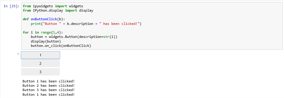
Note- the following might not apply to Notebooks in Pro, but it is good information to know if and when using the stand alone Jupyter Notebook session. Doing this outside of Pro’s Package Manager might corrupt your environment so be sur to perform this on a dedicated env clone.
If you get an error with this code "Failed to display Jupyter Widget of type Button" that means the widgets are probably not installed which we can potentially fix in our Anaconda prompt:
conda install -n base -c conda-forge widgetsnbextension
conda install -n AC37 -c conda-forge ipywidgets
After installing the packages, exit your Jupyter notebook and restart it and try to re-run your code. It is possible you will receive the error again as the widget tries to run before the Javascript library that runs the widgets has opened. In that case try to select your code, wait a few more seconds and then click Run.
If you are still getting an error, it is likely that your packages did not install properly (or in a way that Jupyter/Anaconda could find them). The fix for this is to close Jupyter Notebook, return to Anaconda Navigator, click Environments (on the left), choose your environment and then search for "ipy", you may need to either change the "Installed" dropdown to "Not Installed" if they are missing or perhaps they should be updated (by clicking on the upward point arrow or the blue text).

It is easy to imagine how this example could be extended to provide some choices on how the next analysis step in a longer Data Science project should be performed. Similarly, a slider or text input field could be used to allow the notebook user to change the values of important input variables.
Lesson content developed by Jan Wallgrun and James O’Brien
Autocompletion, Restarting the Kernel, and other useful things
Let’s close this brief introduction to Jupyter with a few more things that are good to know when starting to write longer and more complex notebooks. Like normal development environments, Juypter has an autocomplete feature that helps with the code writing and can save a lot of typing: while editing code in a code cell, you can press the TAB key and Jupyter will either automatically complement the name or keyword you are writing or provide you with a dropdown list of choices that you can pick from. For instance, type in soup.ge and then press TAB and you get the list of options, as shown in Figure 3.13 including the get_text() function that we used in our code.

Another useful keyboard command to remember is SHIFT+TAB. When you place the cursor on a variable name or function call and press this key combination, a window will open up showing helpful information like the type of the variable and its current content or the parameters of the function as in Figure 3.14. This is of great help if you are unsure about the different parameters of a function, their order or names. Try out what you get when you use this key combination for different parts of the code in this notebook.

As in all programming, it may occasionally happen that something goes completely wrong and the execution of the code in a cell won’t terminate in the expected time or not at all. If that happens, the first thing to try is to use the “Interrupt Kernel” button located to the right of the “Execute cell” button. This should stop the execution of the current cell and you can then modify the code and try to run the cell again. However, sometimes even that won’t help because the kernel has become unresponsive. In that case, the only thing you can do is restart the kernel using the “Restart Kernel” button to the right of the “Interrupt Kernel” button. Unfortunately, that means that you will have to start the execution of the code in your notebook from the beginning because all imports and variable assignments will be lost after the restart.
Once you have finished your notebook, you may want to publish or share it. There are many options by wich to do so. In the File menu, there exists the “Download as…” option for obtaining versions of your notebook in different formats. The .ipynb format, as we mentioned, is the native format in which Jupyter saves the notebooks. If you make the .ipynb file available to someone who has access to Juypter, that person can open the notebook and run it or modify the content. The .py option allows for exporting content as a Python script, so that the code can be run outside of Jupyter. If you want a version of your notebook that others can read even without access to Jupyter, there are several options like exporting the notebook as HTML, as Latex, or as PDF. Some of these options require additional software tools to be installed on your computer and there are some limitations. For instance, if you export your notebook as HTML to add it to your personal web page, interactive widgets such as the interactive web map will not be included.
To close this section, we want to again refer to the links we provided at the beginning of this section if you want to keep reading about Jupyter and learn tricks that we weren't able to cover in this brief introduction.
Lesson content developed by Jan Wallgrun and James O’Brien
Practice Exercises
The goal of this exercise is to practice creating GUIs a little bit more. Your task is to implement a rudimentary calculator application for just addition and subtraction that should look like the image below:

The buttons 0… 9 are for entering the digits into the line input field at the top. The buttons + and - are for selecting the next mathematical operation and performing the previously selected one. The = button is for performing the previously selected operation and printing out the result, and the “Clear” button is for resetting everything and setting the content of the central line edit widget to 0. At the top of the calculator we have a combo box that will list all intermediate results and, on selection of one of the entries, will place that number in the line edit widget to realize a simple memory function.
Here is what you will have to do:
- Create the GUI for the calculator with QT Designer using the “Widget” template. This calculator app is very simple so we will use QWidget for the main window, not QMainWindow. Make sure you use intuitive object names for the child widgets you add to the form. (See Sections 2.6.2 and 2.7.2)
- Compile the .ui file created in QT Designer into a .py file (Sections 2.6.2 and 2.7.2).
- Set up a main script file for this project and put in the code to start the application and set up the main QWidget with the help of the .py file created in step 2 (Sections 2.6.1 and 2.7.3).
Hint 1: To produce the layout shown in the figure above, the horizontal and vertical size policies for the 10 digit buttons have been set to “Expanding” in QT Designer to make them fill up the available space in both dimensions. Furthermore, the font size for the line edit widget has been increased to 20 and the horizontal alignment has been set to “AlignRight”.
This is the main part we want you to practice with this exercise. You should now be able to run the program and have the GUI show up as in the image above but without anything happening when you click the buttons. If you want, you can continue and actually implement the functionality of the calculator yourself following the steps below, or just look at the solution code showing you how this can be done.
- Set up three global variables: intermediateResult for storing the most recent intermediate result (initialized to zero); lastOperation for storing the last mathematical operation picked (initialized to None); and numberEntered for keeping track of whether or not there have already been digits entered for a new number after the last time the +, -, = or Clear buttons have been pressed (initialized to False).
- Implement the event handler functions for the buttons 0 … 9 and connect them to the corresponding signals. When one of these buttons is pressed, the digit should either be appended to the text in the line edit widget or, if its content is “0” or numberEntered is still False, replace its content. Since what needs to happen here is the same for all the buttons, just using different numbers, it is highly recommended that you define an auxiliary function that takes the number as a parameter and is called from the different event handler functions for the buttons.
- Implement an auxiliary function that takes care of the evaluation of the previously picked operation when, e.g., the = button is clicked. If lastOperation contains an operation (so is not None), a new intermediate result needs to be calculated by applying this operation to the current intermediate result and the number in the line edit widget. The new result should appear in the line edit widget. If lastOperation is None, then intermediateResult needs to be set to the current text content of the line input widget. Create the event handler function for the = button and connect it to this auxiliary function.
- Implement and connect the event handler functions for the buttons + and - . These need to call the auxiliary function from the previous step and then set lastOperation to a string value representing the new operation that was just picked, either "+" or "-".
- Implement and connect the event handler for the “Clear” button. Clicking it means that the global variables need be re-initialized as in step 4 and the text content of the line edit widget needs to be set back to “0”.
- Implement the combo box functionality: whenever a calculation is performed by the auxiliary function from step 6, you now also need to add the result to the item list of the memory combo box. Furthermore, you need to implement and connect the event handler for when a different value from the combo box is picked and make this the new text content of the line edit field. The signal of the combo box you need to connect to for this is called “activated”.
Practice Exercise solution
The image below shows the hierarchy of widgets created in QT Designer and the names chosen. You can also download the .ui file and the compiled .py version here [37] and open the .ui file in QT Designer to compare it to your own version. Note that we are using a vertical layout as the main layout, a horizontal layout within that layout for the +, -, =, and Clear button, and a grid layout within the vertical layout for the digit buttons.

The following code can be used to set up the GUI and run the application but without yet implementing the actual calculator functionality. You can run the code and main window with the GUI you created will show up.
import sys
from PyQt5.QtWidgets import QApplication, QWidget
import calculator_gui
# create application and gui
app = QApplication(sys.argv)
mainWindow = QWidget()        # create an instance of QWidget for the main window
ui = calculator_gui.Ui_Form() # create an instance of the GUI class from calculator_gui.py
ui.setupUi(mainWindow)        # create the GUI for the main window
# run app

mainWindow.show()
sys.exit(app.exec_())
The main .py file for the full calculator can be downloaded here [38]. Function digitClicked(…) is the auxiliary function from step 5, called by the ten event handler functions digitPBClicked(…) defined later in the code. Function evaluateResult() is the auxiliary function from step 6. Function operatorClicked(…) is called from the two event handler functions plusPBClicked() and minusPBClicked(), just with different strings representing the mathematical operation. There are plenty of comments in the code, so it should be possible to follow along and understand what is happening rather easily.
Lesson 4 Assignment
In this homework assignment, we want you to create a script tool or Jupyter Notebook (using Pro’s base environment).
You can use a previous lesson assignment’s script, or you can create a new one that is pertinent to your work or interest. If you choose to do the later, include a sample dataset that can be used to test your script tool or Jupyter Notebook and include in your write-up the necessary steps taken for the script tool or Notebook to work.
Write-up
Produce a 400-word write-up on how the assignment went for you; reflect on and briefly discuss the issues and challenges you encountered and what you learned from the assignment.
Deliverable
Submit a single .zip file to the corresponding drop box on Canvas; the zip file should contain:
- Your script file
- Your 400-word write-up