Lesson 3: Reservoir Engineering: Rock and Fluid Properties
3.0: Lesson Overview
You will have two weeks to complete Lesson 3.
Lesson 3 is very extensive, and you will have two weeks to read through the lesson and complete the associated assignments. Please use your time wisely and don't let yourself fall behind; you will need the extra week to work your way effectively through the material.
Please refer to the Calendar in Canvas for specific time frames and due dates.
Overview
Petroleum engineers working in the upstream sector of the oil and gas industry must perform their analyses on the known properties of the reservoirs and reservoir fluids associated with the oil and gas fields they are tasked to manage. The properties that these petroleum professionals are most likely to use during their careers are:
- Rock properties
- Fluid properties
- Oil properties
- Gas properties
- Water properties
- Rock-Fluid interaction properties
These data are required for most routine calculations and are typically obtained with field or laboratory measurements. In cases where these data are unavailable due to time or cost constraints, industry accepted correlations are available for generating missing data. For detailed analyses, measured data are preferred; however, data from correlations serve a vital role of generating data for quick, low cost analyses. In this lesson, we will discuss the data used in petroleum engineering analyses. We will discuss what data are available, how the data are used in the field, how the data are measured in the field or laboratory, and what correlations are available to supplement missing data.
Learning Objectives
By the end of this lesson you should be able to:
- identify the units used in the oil and gas industry;
- list the data used by petroleum engineers on a daily basis during their careers;
- list the sources (field, laboratory, or derived from correlations) of these data;
- explain the basics of the field and laboratory procedures used to obtain these data;
- list and discuss the assumptions behind the field and laboratory measurements;
- calculate required data from raw laboratory or field measurements;
- calculate required data from industry standard correlations;
- describe the relationships and dependencies of the data;
- integrate rock, fluid, and rock-fluid interaction data to perform basic analyses, such as storage and flow rate calculations; and
- discuss the concept of fluid saturations and how these saturations impact storage and production of oil and gas.
Lesson 3 Checklist
| To Read | Read the Lesson 3 online material | Click the Oilfield Measures and Units link below to continue reading the Lesson 3 material |
|---|---|---|
| To Do | Lesson 3 Problem Set | Submit your solutions to the Lesson 3 Problem Set assignment in Canvas |
Please refer to the Calendar in Canvas for specific time frames and due dates.
Questions?
If you have questions, please feel free to post them to the Course Q&A Discussion Board in Canvas. While you are there, feel free to post your own responses if you, too, are able to help a classmate.
3.1: Oilfield Measures and Units
The domestic United States oil and natural gas industry uses a very specific set of measures and units that were common at the dawn of the industry and, at least in the U.S., have been retained and expanded upon over the years. These units are often called Oilfield Units. In the international oil and gas industry, the metric system or the related S.I. (Systeme Internationale) system are used. In this course, we will use the U.S. domestic, oilfield units.
The standard measure of volume in the U.S. oil and gas industry is the Barrel (bbl) for liquids and the cubic foot (ft3) for gases. The barrel is defined as 42 U.S. gallons. That is:
You have probably noticed that the unit for barrel, “bbl,” has two “b’s”, while the word for barrel only has one. One story relating the origin of the unit “bbl” and the measure of 42 U.S. gallons follows[2]:
In the early 1860s, when oil production began, there was no standard container for oil, so oil and petroleum products were stored and transported in barrels of all different shapes and sizes (beer barrels, fish barrels, molasses barrels, turpentine barrels, etc.). By the early 1870s, the 42-gallon barrel had been adopted as the standard for oil trade. This was 2 gallons per barrel more than the 40-gallon standard used by many other industries at the time. The extra 2 gallons was to allow for evaporation and leaking during transport [sic] (most barrels were made of wood). Standard Oil began manufacturing 42 gallon barrels that were blue to be used for transporting petroleum. The use of a blue barrel, abbreviated "bbl," guaranteed a buyer that this was a 42-gallon barrel.
In August of 1866, independent American oil producers met in Titusville, PA and agreed that the 42 gallon barrel would be the industry standard in the U.S.A. [3]
Because of the slightly compressible nature of liquids and the compressible nature of gases, the volume of a given mass of liquid or gas at one set of pressure and temperature conditions will not equal the same volume at a different set of pressure and temperature conditions. To provide a common measure of volume, we can specify the volume of a given mass measured at a reference pressure and temperature.
For liquids, the Upstream Oil Industry uses the pressure and temperature at Stock Tank Conditions as the reference conditions for discussing standardized volumes. The stock tank is the last vessel used in the field separation of crude oil and natural gas prior to the transport to other field processing plants (local oil or gas plants) or export to a distant refinery. The Stock Tank Pressure and Stock Tank Temperature make up a field dependent set of conditions which are determined by the pressure and temperature that maximizes the volume of the produced oil. In other words, a crude oil with a specific composition is produced from a reservoir and the field Separator and Stock Tank conditions are adjusted to maximize the volumetric yield of the crude oil. The pressure and temperature conditions that maximize the crude oil volume from one reservoir will be different from the pressure and temperature conditions that maximize the crude oil volume from another reservoir due to the difference in the crude oil compositions. Thus, the stock tank pressure and stock tank temperature in one oilfield may be different from the stock tank pressure and stock tank temperature in another oilfield. Representative stock tank conditions may be on the order of 100 psi and 75°F. Figure 3.02 shows a typical, three-stage, gas-oil Separation Train.
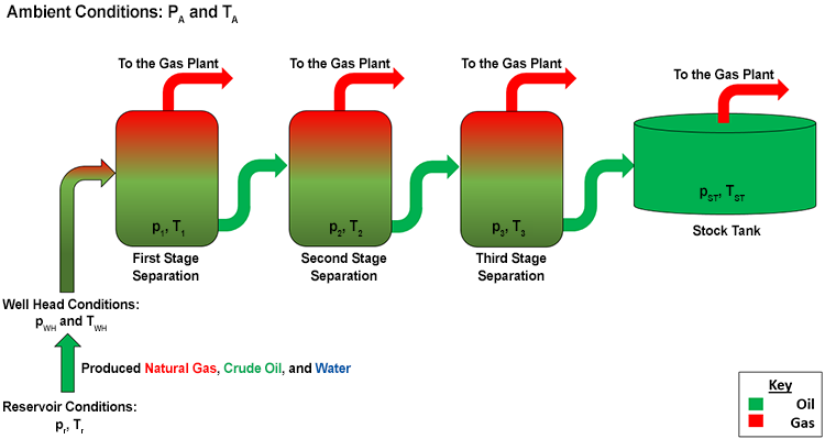
In this figure, the stock tank pressure and temperature, pST and TST, are the field-specific reference pressure and temperature used in all reservoir engineering calculations for crude oil and produced water. When referring to liquid volumes at stock tank conditions, we use the units of Stock Tank Barrels (STB).
For gases, we use Standard Conditions, pSC and TSC, as the reference conditions for volumetric reservoir engineering calculations. Standard conditions are defined by different governments, scientific agencies, industries, or in some instances, specific legal contracts. The Society of Petroleum Engineers (SPE) defines these conditions as pSC = 14.696 psi (101.325 kPa) and 59°F (15°C). Informally, many engineers use pSC = 14.7 psi and 60°F. The appropriate set of standard conditions to be used in engineering calculations will often be dictated by the company and the location where the engineer works. When referring to the gas volumes at standard conditions, we use the units of Standard Cubic Foot (SCF).
For volumetric rate calculations, the U.S. oil and gas industry uses the symbol “q” for the volume of oil or gas produced (or transported) over a 24-hour period. Thus, we have:
- qo = STB/day for oil (at stock tank conditions)
- qw = STB/day for water (at stock tank conditions)
- qg = SCF/day for gas (at standard conditions)
When we consider volumes at a field scale, we often need to use units greater than the stock tank barrel, STB, or the standard cubic foot, SCF. For this, the oil industry uses the uppercase letter “M.” This stands for thousands of STB or SCF. For example, the unit of MSTB refers to thousands of STBs, and the unit of MSCF refers to thousands of SCF. Likewise, the unit of MMSTB refers to millions of STBs, and the unit of MMSCF refers to millions of SCF.
| 1 MMSTB | = 1,000 MSTB | = 1,000,000 STB |
| 1 MMbbl | = 1,000 Mbbl | = 1,000,000 bbl |
| 1 MMSCF | = 1,000 MSCF | = 1,000,000 SCF |
| 1 MM ft3 | = 1,000 M ft3 | = 1,000,000 ft3 |
| 1 MMSTB/day | = 1,000 MSTB/day | = 1,000,000 STB/day |
| 1 MMSCF/day | = 1,000 MSCF/day | = 1,000,000 SCF/day |
[2] Source: Seeking Alphaα - Where Does That 2nd 'B' in the Abbreviation for Crude Barrels (BBL) Come From? [1]
[3]Source: American Oil & Gas Historical Society - History of the 42-Gallon Oil Barrel [2]
3.2: Reservoir Rock Properties
The reservoir rock properties that are of most interest to development geologists and reservoir engineers (amongst others) are Porosity, Compressibility, and Permeability. Porosity is a rock property that defines the fraction of the rock volume that is occupied by the pore volume. Compressibility is the rock property that governs the relative change in the pore volume when pressure is either increased or decreased. Finally, permeability is the rock property that is a measure of the ease (or difficulty) with which liquids or gases can flow through a porous medium.
Rock Porosity
As previously mentioned, porosity, ϕ, is the fraction of the Bulk Rock Volume, , that is occupied by the Pore Volume, . Mathematically, it is defined as:
The bulk volume, Vb, can also be defined as the sum of the volumes of the two constituents of the rock, pore volume and Grain Volume, Vg. That is:
From these two expressions, we can develop several equivalent definitions for porosity:
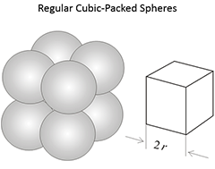
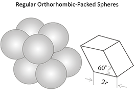
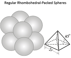
Figure 3.03 (below) shows the porosities for three different idealized grain packings. In this figure, the rock grains are the spheres and the pore volume is the space between the spheres. Note that the porosities of these three systems are independent on the radii of the grains. In a real rock, the grains would be angular (if quartz grains in sandstones) and some of the void space might be filled with smaller grains, mineral cementation, and clays.
 |
|
 |
|
 |
At this point, we must distinguish between two types of porosity in rock: Total Porosity, , and Effective Porosity, . Real reservoir rock is comprised of connected pores and isolated pores. As the name implies, connected pores are pores which are connected to other pores and are capable of transmitting fluids. Isolated pores are pores, or groups of pores, which do not connect to other pores or form dead-end pathways. These isolated pores are incapable of transmitting fluids. Total porosity is defined as the total pore space (connected plus isolated pores) divided by the bulk volume, while effective porosity is the connected pore volume divided by the bulk volume.
Reservoir engineers are concerned with how fluids are stored and flow in the reservoir. Consequently, reservoir engineers are more concerned with effective porosity,
The porosity is of primary concern to geologists and reservoir engineers because it is a direct measurement of the ability of a reservoir rock to store fluids. There are two ways that oil and gas professionals can obtain measurements of porosity through laboratory measurement and through the use of Well Logs.
3.2.1: Porosity from Laboratory Measurements
One method in which porosity is determined is by laboratory measurements of Core Samples brought to the surface during drilling. Measurement of porosity in the laboratory is part of Routine Core Analysis, sometimes referred to as PKS Analysis (porosity, permeability, and saturation analysis).
Core samples are rock samples that are cut from the reservoir formation using specialized Coring Bits. The extraction of core samples is a very complicated process and requires a lot of planning. When cutting a core, all phases of the coring process must be considered to ensure that the porosity is not altered prior to its delivery to the laboratory. These phases include core cutting, core handling, core preservation, core transport, core sampling, and core testing. Typically, a Formation Evaluation Specialist takes the lead role in designing the core program while working with a development geologist, a reservoir engineer, and a drilling engineer.
After retrieving representative core samples and delivering them to the laboratory, there are several methods that can be used to determine porosity. As shown in Equations 3.01 through 3.03, to determine porosity, we need to determine two of the three volumes, , , or . Once these are determined, then the porosity and the third volume are known.
Bulk Volume, , Determination
Bulk volume can be determined by one of two methods, physical measurement and displacement. The use of physical measurements is only applicable to core samples with regular geometric shapes. As the name implies, physical measurement involves the measurement of the dimensions of the core sample (typically a cylindrical core plug) and calculating the volume from standard volumetric formulae.
Displacement methods involve the immersion of the core sample in mercury inside of a pycnometer or graduated cylinder. Mercury is used in displacement methods to prevent invasion into the pore space. The bulk volume of the sample is the apparent volume change of the mercury in the pycnometer or graduated cylinder. Alternative, Archimedes’ Principle can be used to determine the bulk volume of the core sample from the apparent weight change due to buoyancy when fully immersed.
Grain Volume, , Determination
The most direct method for determining grain volume is to measure the weight of a dried sample and to divide by the density of the rock matrix. Unfortunately, the rock densities are often not accurately known.
A second method, similar to the immersion method for bulk volume determination, can be used for grain volume determination. In this method, a core sample is crushed and the resulting rock grains are placed into a pycnometer or graduated cylinder along with a known volume of liquid. The volume of the rock grains can then be determined from the apparent volume change of the liquid (the Russell Method) after immersion or the apparent weight change (the Melcher-Nutting Method) of the immersed sample due to buoyancy using Archimedes’ Principle.
Unfortunately, the disadvantage of this method is that it is destructive. Once the sample is pulverized, it cannot be used for further testing. Since we have crushed the core sample to its constituent rock grains, the porosity determined from the immersion of these grains is the total porosity, .
A third method is the Boyle’s Law Method. As the name implies, it uses Boyle’s Law for the grain volume determination:
In this method, the core sample is placed into one chamber of an experimental apparatus containing two chambers of known volume connected by a closed valve. An inert gas (helium or nitrogen) is introduced into the chambers at different, but known, pressures. At this point, the total number of moles, nT, in the apparatus can be determined from:
For isothermal conditions, this reduces to Boyle’s Law:
The valve between the chambers is opened and the pressure is allowed to stabilize to the final pressure, pf, and is recorded. If we assume that the core sample was placed into Chamber 1, then we have:
Example 3.01
Given the following data:
- Weight of the crushed core sample in air:
- Weight of the crushed core sample in water:
- Density of water:
Use Archimedes’ Principle to calculate the grain volume of the sample.
SOLUTION:
The weight of the displaced water is simply the apparent change in weight of the sample due to buoyancy:
The volume of the rock grains then becomes the volume of the displaced water:
Solving for :
The advantages of this method are that it is non-destructive and can be very accurate. The disadvantage of this method is that for low permeability core samples, it may take a long time for the pressures to stabilize. Since the gases can only enter or leave the connected pores, the porosity obtained from the Boyle’s Law Method is the effective porosity, .
Pore Volume, , Determination
Early methods used for pore volume determination, such as the Washburn-Bunting Method, used mercury injection into the pore spaces of the core sample. In these Mercury Injection Methods, high pressure mercury was injected into the core sample and the volume of mercury entering the core was measured. These methods had several drawbacks, including the destructive nature of the test and the compression of any gases in the core sample retaining a residual volume, resulting in measurement inaccuracies.
Example 3.02
Given the data:
When the valve between Chamber 1 and Chamber 2 is opened, the pressure is found to stabilize at . What is the grain volume of the core sample?
SOLUTION:
From Equation 3.10, we have:
A second method, the Resaturation Method, uses a clean dry core sample and resaturates it with a fluid of known density. The change in weight of the sample can then be used to determine the pore volume, Vp, of the sample
Since the fluid can only enter or leave the connected pores, the porosity obtained from the resaturation method is the effective porosity, .
A third method for the determination of the pore volume is the Summation of Fluids Method. In this method, a core sample in its native state (not cleaned or dried) is halved. In one of the halves, mercury injection is used to estimate the gas volume, while the second half is used in the retorting (distillation) process to determine the oil and water volumes. The pore volume is then set equal to the sum of the fluid volumes. The advantage of this method is that the Phase Saturations (fraction of the pore space occupied by each phase – oil, gas, and water) can be determined simultaneously with the porosity. The disadvantages of the method are the destructive nature of the test and the assumption that both halves of the core sample contain similar fluid volumes.
Again, in the summation of fluids method, fluids can only enter or leave the connected pores. Consequently, the porosity obtained from this method is the effective porosity, .
Example 3.03
Given the following data:
- Weight of the clean dried core sample in air:
- Weight of the core sample saturated with water:
- Density of water:
What is the pore volume of the core sample?
SOLUTION:
The weight of the water saturating the sample is:
The pore volume of the core sample then becomes the volume of the water saturating the core:
| Method | Porosity Type | Advantages | Disadvantages |
|---|---|---|---|
| Grain Determination by Immersion | Total Porosity, |
|
|
| Grain Determination by Boyles Law | Effective Porosity, |
|
|
| Washburn-Bunting (Mercury Injection) | Effective Porosity, |
|
|
| Resaturation | Effective Porosity, |
|
|
| Summation of Fluids | Effective Porosity, |
|
|
3.2.2: Porosity from Well Logs
The most common method of determining porosity is with Well Logs. Well logs are tools sent down the wellbore during the drilling process which measure different reservoir properties of interest to geologists and engineers. Due to the expense of obtaining core samples, typically only a few wells are cored. The wells that do get cored are usually wells early in the life of the reservoir (appraisal wells) and key wells throughout the reservoir. On the other hand, well logs are routinely run in wells, if only to identify the depths of the productive intervals. The three open-hole logs used to evaluate porosity are:
- The sonic log
- The density log
- The neutron log
While none of these logs measures porosity directly, the porosity can be calculated based on theoretical or empirical considerations. The measurements obtained from these logs are not only dependent on the porosity but are also dependent on other rock properties such as:
- Lithology (rock type: sandstone, limestone, shale, etc.)
- The fluids occupying the pore spaces
- The wellbore environment (type of drilling fluid, hole size)
- The geometry of the pores
Since many variables may impact the log readings, corrections need to be applied to the log interpretations and the three logs are typically evaluated together to determine the best estimate of the porosity of rock formations. The log evaluations are also calibrated against core porosity in wells where both core and logs are available.
The Sonic Log measures the acoustic transit time, Δt, of a compressional sound wave traveling through the porous formation. The logging tool consists of one or more transmitters and a series of receivers. The transmitters act as sources of the acoustic signals which are detected by the receivers. The time required for the signal to travel through one foot of the rock formation is the acoustic transit time, Δt. The acoustic travel time, then, is the reciprocal of the sonic velocity through the formation. The units of Δt are micro-seconds/ft (μsec/ft) or millionths of a second per foot.
There are several ways to interpret the sonic log measurements. One of the most common interpretation formulae is the Wyllie Time-Average Equation:
Where:
- ϕsl is the porosity from the sonic log (log measurement) , fraction
- Δtsl is value of the acoustic transit time measured by the sonic log, μsec/ft
- Δtma is value of the acoustic transit time of the rock matrix measured in the laboratory, μsec/ft
- Δtf is value of the acoustic transit time saturating fluid measured in the laboratory, μsec/ft
The presence of hydrocarbons in the reservoir rock results in an over prediction of porosity measured by the sonic log and some corrections may be required. These corrections take the form:
or,
Table 3.03 has typical values of the acoustic transit time for different reservoir formations and commonly encountered reservoir fluids.
| Heading1 | Δtma (μsec/ft) Range |
Δtma (μsec/ft) Commonly Used |
Δtf (μsec/ft) Range |
Δtf (μsec/ft) Commonly Used |
|---|---|---|---|---|
| Sandstone | 55.5 – 51.0 | 55.5 or 51.0 | — | — |
| Limestone | 47.8 – 43.5 | 47.5 | — | — |
| Dolomite | 43.5 | 43.5 | — | — |
| Anhydrite | 50.0 | 50.0 | — | — |
| Salt Formation | 66.7 | 67.0 | — | — |
| Fresh Water Based Drilling Fluid |
— | — | 189.0 | 189.0 |
| Salt Water Based Drilling Fluid |
— | — | 185.0 | 185.0 |
| Gas | — | — | 920.0 | 920.0 |
| Oil | — | — | 230.0 | 230.0 |
| Casing (Iron) | — | — | 57.0 | 57.0 |
Other empirically based equations exit for sonic log interpretation. One form of an alternative equation is:
In this equation, the value of C is in the range of 0.625 to 0.700 and is determined by calibrating the equation to known porosity, such as, to core data when a well is both cored and logged. In Equation 3.12 and Equation 3.13, ϕsonic is the final interpreted porosity from the sonic log.
The Density Log measures the electron density ρe, of the formation (the electron density is the number of electrons per unit volume). The density logging tool emits gamma rays from a chemical source which interact with the electrons of elements in the formation. Detectors in the tool count the returning gamma rays. These returning gamma rays are related to the election density of the elements in the formation.
The electron density is proportional to the bulk density, ρb, of the formation (the bulk density is the density of the fluid-filled rock in grams per unit volume). For a molecular substance, this proportionality is:
Where:
- is the electron density of the formation, electrons/cc
- is the bulk density of the formation, gm/cc
- ΣZ is the sum of the atomic numbers making up the molecule, electrons/molecule
- MW is the molecular weight, gm/molecule
Table 3.04 contains the term in the parenthesis for common substances related to oil and gas production.
| Compound | Chemical Formula |
Actual Density, (gm/cc) |
(electrons/gm) |
Electron Density, (electrons/cc) |
Log Reading, Apparent (gm/cc) |
|---|---|---|---|---|---|
| Quartz | SiO2 | 2.654 | 0.9985 | 2.650 | 2.648 |
| Calcite | CaCO3 | 2.710 | 0.9991 | 2.708 | 2.710 |
| Dolomite | CaCO3MgCO3 | 2.870 | 0.9977 | 2.863 | 2.876 |
| Anhydrite | CaSO4 | 2.960 | 0.9990 | 2.957 | 2.977 |
| Sylvite | KCl | 1.984 | 0.9657 | 1.916 | 1.863 |
| Halite | NaCl | 2.165 | 0.9581 | 2.074 | 2.032 |
| Gypsum | CaSO42H2O | 2.320 | 1.0222 | 2.372 | 2.351 |
| Anthracite Coal | --- | 1.400 - 1.800 | 1.0200 | 1.442 – 1.852 | 1.355 – 1.796 |
| Bituminous Coal | --- | 1.200 - 1.500 | 1.0600 | 1.227 – 1.590 | 1.173 – 1.514 |
| Fresh Water | H2O | 1.000 | 1.1101 | 1.110 | 1.000 |
| Brine (200,000 ppm) | --- | 1.146 | 1.0797 | 1.237 | 1.135 |
| Oil | N(CH2) | 0.850 | 1.1407 | 0.970 | 0.850 |
| Methane | CH4 | 1.2470 | 1.247 | 1.335 - 0.1883 | |
| Gas | --- | 1.2380 | 1.238 | 1.238 - 0.1883 |
One important observation from this table is that the column containing the group in parenthesis in Equation 3.14, , is approximately 1.0. Since this term is close to unity, the electron density is a very close approximation to the bulk density, as also seen in Table 3.03. The logging tool is calibrated by running it against a limestone formation containing fresh water. With this calibration, the Log Reading, Apparent ρba (last column in Table 3.03) is:
For some substances, such as liquid-filled sandstones, limestones, and dolomites, ρba can be used directly as ρb. For other substances, such as sylvite, rock salt, gypsum, anhydrite, coal, and gas bearing formations, further corrections are required. These additional corrections are beyond the scope of this course. Once the bulk density is determined, the porosity can be estimated by:
Where:
- ϕdensity is the final interpreted porosity from the density log, fraction
- ρma is the matrix density (from the Actual Density, ρb, Column in Table 3.03), gm/cc
- ρb is bulk density from density log (Equation 3.15), gm/cc
- ρf is the density of the fluid measured in the laboratory, gm/cc
The Neutron Log measures the amount of hydrogen in the formation being logged. Since the amount of hydrogen per unit volume is approximately the same for oil and water, the neutron log measures the Liquid Filled Porosity (the porosity excluding the Gas-Filled Porosity). The neutron logging tool emits neutrons from a chemical source which collide with nuclei of elements in the formation. The element in the formation with the mass closest to a neutron is hydrogen. Due to the parity in mass, the neutron in a neutron-hydrogen collision loses approximately half of its energy. With enough collisions, the neutron eventually loses enough energy and is absorbed by the hydrogen nucleus and a gamma ray is emitted. The neutron logging tool measures these emitted gamma rays. Note, other hydrogen atoms may be present in clays in the rock, or in the rock itself and corrections for these other hydrogen atoms are required.
Interpretation of the neutron log is performed by first calibrating the logging tool to specific well and formation conditions. Interpretation charts supplied by the logging company are used to interpret the log for deviations from these calibration conditions. The interpretation of the neutron log for ϕneutron is beyond the scope of this course.
As mentioned throughout the discussion on porosity logging, due to the various wellbore and formation conditions encountered during the logging operations (i.e., real conditions, as opposed to laboratory conditions) many corrections may be required to get a good interpretation from the different well logs. In addition, the logs are typically evaluated together to aid in the interpretation. Finally, if core data are available from a well, then the core derived porosity is used to calibrate the logging tools.
Rock (Pore-Volume) Compressibility
In addition to the porosity and its relation to pore-volume, reservoir engineers are also interested in how the pore-volume behaves (increases or decreases) with increases or decreases in pore-pressure. The industry standard relationship for change in pore-volume is based on the isothermal pore-volume compressibility, cPV.
The isothermal pore-volume compressibility is always positive and is defined as:
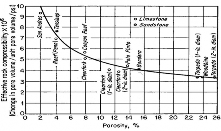
The units of compressibility are 1/psi. Equation 3.17 implies that as pressure increases the pore-volume increases. Hall [4] correlated the effective rock compressibility as a function of porosity which is shown in Figure 3.04.
For a constant bulk volume and compressibility, we can separate variables in Equation 3.17 and integrate to arrive at the following relationship between pore-volume (or porosity) and pore pressure:
or,
Where ϕref is a reference porosity measured at reference pressure, pref. After some manipulation:
To further simplify this relationship, if we assume a small pore-volume compressibility (as shown in Figure 3.03, we are typically dealing with rock compressibilities on the order of 10-6 1/psi) and apply a Taylor Series expansion to the exponential function (truncated after one term), we obtain:
The rock compressibility determination is performed in the laboratory on core samples. The rock compressibility is an expensive test to run and is not part of the Routine Core Analysis. It must be specifically requested as part of any Special Core Analysis, or SCAL, testing performed on the core sample.
Rock Permeability
The permeability of a porous medium is a measure of the ease (or difficulty) in which a fluid can flow through the pores of the medium. Permeability is a property of the porous medium which in our case is the reservoir rock. The unit of permeability is the Darcy, or D, named after the French engineer Henri Darcy who investigated the flow of water through filter beds in the city of Dijon in the mid-1800s. The unit of Darcy has the dimensions of length-squared. One significant contribution from Darcy’s work (among many), is Darcy’s Law, which was published in 1856 and forms one of the foundations of porous media flow:
Where:
- qw is the flow rate of water, cc/sec
- k is the permeability of the medium, Darcy
- A is cross-sectional area, cm2
- l is the length in the direction of flow, ft (x, y, or z in Cartesian coordinates)
- is the pressure gradient, atm/cm
The unit of the Darcy is defined as the permeability, k, required to allow a flow rate, qw, of one cc of water per second through a medium with a cross-sectional area, A, of one cm2, with an applied pressure gradient, Δp/ΔL, of one atm/cm. As it turns out, the Darcy as a unit is too large for most field applications. In reservoir engineering we typically work with the millidarcy, md, which is one one-thousandth of a Darcy:
Henri Poiseuille later generalized Darcy’s Law to fluids other than water by noting that the flow rate was inversely proportional to the dynamic viscosity, μf, of the fluid flowing through the porous medium. The unit of dynamic viscosity, the poise, is named after Poiseuille and is a property of the fluid. Again, as it turns out, the poise as a unit is also too large for most field applications. In reservoir engineering we typically work with the centipoise, cp, which is one one-hundredth of a poise:
The generalized form of Darcy’s Law for any single-phase fluid which incorporates the fluid viscosity is:
Darcy’s Law has several important assumptions associated with it. These include:
- A rigid porous medium (incompressible medium with no transport of rock grains, e.g. fines movement
- An incompressible, homogeneous, Newtonian fluid that fully saturates (single-phase) the porous medium
- Steady-state, isothermal, and laminar (low Reynolds number) flow conditions
- No interactions between the porous medium and the fluid flowing through it
- A no-slip interface between the porous medium and the fluid flowing through it (zero velocity boundary condition at the rock-fluid interface)
The form of Darcy’s Law discussed so far uses the SI unit system. For oilfield units, we have:
Where:
- qf is the flow rate of the saturating fluid, bbl/day
- 0.001127 is a unit conversion constant
- k is the absolute permeability of the medium, md
- A is cross-sectional area, ft2
- is the pressure gradient, psi/ft
Measurement of the permeability can be done through laboratory or field measurements. In the laboratory, a core sample of known dimensions (A and ΔL) is cleaned and placed into a fluid-tight core holder. A fluid of known viscosity (typically air) is allowed to flow through the core at a metered flow rate. Darcy’s Law is then used to calculate the permeability of the core sample.
In the field, permeability is measured with a Well Test using Pressure Transient Analysis. Under certain conditions, the production rate(s) (can be a zero-production rate) results in well pressures that honor known solutions to the Diffusivity (or Well Test) Equation. When the well test results are compared to the solutions to the diffusivity equation, the permeability of the formation can be estimated.
One common well test is a Pressure Build-Up Test. In a pressure build-up test, the well is produced at a stable (constant) rate, qp, for a production time of tp. The well is then shut in and the pressure is monitored during the shut-in period Δt; where Δt is measured from the beginning of the well is shut-in. The well test is called a build-up test because when the well is shut in, the pressures increase with increasing Δt. One analysis tool for the pressure build-up test is the Horner Plot. A typical Horner plot is shown in Figure 3.05.
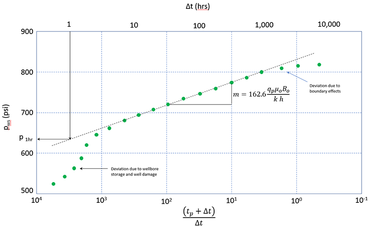
In this plot shown in Figure 3.05, pws are the shut-in well pressures measured during the well test, tp and Δt are times in hours (Δt measured from the time that the well is shut-in), qp is the stabilized production rate during the production period prior to well shut-in in STB/day, μo is the oil viscosity in cp, Bo is the Formation Volume Factor in bbl/STB, k is the permeability in md, and h is the reservoir thickness in ft.
In a Horner Plot, the function , decreases as increases. As can be seen in this figure, the slope of the Horner Plot is related to the permeability of the reservoir near the well. If the shut-in pressures, pws, are measured and the slope calculated, then the permeability can be determined if all the other parameters in the definition of the slope are known.
In semi-logarithmic plots (plots with one conventional axis and one logarithmic axis), such as that in Figure 3.05, the slope is normally taken over one logarithmic cycle. That is:
While there is no universal correlation between permeability, field measurements suggest that as the porosity of a formation increases, the permeability of the formation also increases. This behavior is captured in a permeability-porosity cross-plot. One such example of a permeability-porosity cross plot is illustrated in Figure 3.06.
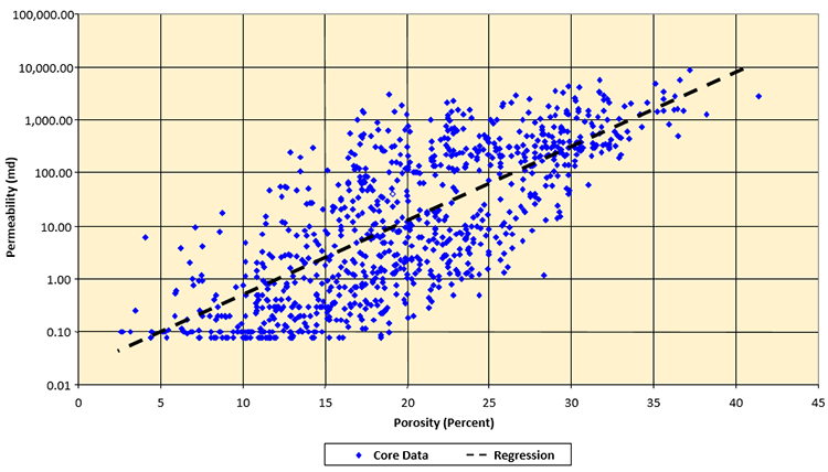
A permeability-porosity cross-plot is a field dependent transform that relates core derived permeability to core derived porosity. Note that the permeability-porosity transform shown in Figure 3.06 is plotted on a semi-logarithmic plot with the permeability plotted on the logarithmic scale. Also note that in the middle of the plot (ϕ = 20 percent) there is an approximate four order of magnitude error bar in the permeability data. This is typical for a permeability-porosity transform. While the results from these transforms may be crude, they are often the only source of permeability data when building complex models of oil or gas reservoirs. Note, geologists have developed methods for capturing this scatter into their models in the form of Scatter Plots, but the development of such plots is beyond the scope of this course.
The permeability in the presence of a single-phase fluid is called the absolute permeability. Since we will be dealing with multi-phase flow, we will need to discuss extensions to Darcy’s which allow for more than one phase. We will do this later in this lesson when we discuss Reservoir Rock-Fluid Interaction Properties.
3.3: Reservoir Fluid Properties
Reservoir fluid properties are normally measured in the laboratory. Pressure-Volume-Temperature (PVT) properties relate these properties to each other at equilibrium conditions. These variables, typically used for volumetric related reservoir behavior, are measured in a laboratory PVT Cell. A PVT Cell is a high-pressure vessel (container) that allows for the control and measurement of pressure, volume, and temperature.
In addition to laboratory measurements, reservoir PVT properties can be determined from Equations-of-State (EOS). Equations-of-state are theoretically derived equations that relate the State Variables: pressure, volume, and temperature (state variables are variables that define the thermodynamic state of a system). Three common examples of equations-of-state include:
Isothermal compressibility:
Real gas law:
Van der Waal’s Cubic EOS:
In Equation 3.26, the negative sign is required because the volume of a fluid decreases as pressure increase (i.e., the derivative is negative). Note that all of these relationships allow for the determination of one of the state variables, p, V, or T, if the two other variables are known (two degrees of freedom). For the isothermal compressibility EOS, Equation 3.26, temperature can be considered a variable if we have tables or equations where the value of cf can be defined for a specific temperature.
In addition to the equations-of-state, fluid PVT correlations are also used in the oil and gas industry. These correlations can be either graphical or mathematical in nature. Fluid property correlations are simply plots, curve fits, or regressions of many laboratory measurements covering a wide range of data. In general, these correlations may not be as accurate as laboratory measurements or equations-of-state, but they have their uses in reservoir engineering.
3.3.1: Water Properties
All oil and gas reservoirs have water associated with them. Since it is a common part of the system, we will need to discuss how it is stored and moves in the reservoir.
Water Formation Volume Factor, Bw
The water (or more correctly, the brine) Formation Volume Factor, Bw, (sometimes referred to as the FVF) is a pressure and temperature dependent property that relates the volume of 1.0 stock tank barrel, STB, of water to its volume in barrels, bbl, at another pressure. It has the units of bbls/STB. We have already discussed the use of the stock tank pressure and temperature as an oilfield reference system.
By definition, if we had 1.0 STB of water at pST and TST, and that same STB occupied 1.02 bbls at reservoir conditions, pr and Tr, then it would have a formation volume factor of:
We can also define the formation volume factor in terms of densities at stock tank conditions and at reservoir conditions. If we assume the mass of 1.0 STB, m1 STB, then at reservoir conditions, we would have:
which implies:
Water Isothermal Compressibility, cw
Water is considered to be a slightly compressible liquid with a very low value of compressibility. From Equation 3.26 we have:
One correlation for water compressibility[5] , cw, is:
Where:
- p is the pressure, psi
- C is the salt concentration, gm/L
- T is temperature, °F
We can develop an explicit formula for the water formation volume factor based on the water compressibility. If we take 1.0 STB of water and its volume in barrels at a reservoir pressure and temperature, then we would have: Vw (bbl) = Bw (pr, Tr) (bbl/STB) x 1.0 STB. Now,
or,
Water Viscosity, μw
In the laboratory, the water viscosity is measured with an apparatus called a Viscometer. The mechanics and test procedures for a viscometer are beyond the scope of this course, and we will work with known correlations. One correlation from McCain has the form:
with
and
where
- μw 14.7 psi is the water viscosity at 14.7 psi and temperature, T °F
- S is the salt concentration in weight percent, Wt% (note different unit from Equation 3.31)
Once the viscosity at 14.7 psi and T °F are determined, the water viscosity at other pressures can be determined from:
Water Density, ρw
The density of water is also a property of interest in petroleum engineering. McCain[6] provides the following correlation for estimating the water density at reference conditions:
where
- ρw ST is the water density at sock tank conditions, lb/ft3
- S is the salt concentration in weight percent, Wt%
The water density at reservoir conditions can then be calculated using Equation 3.29.
[5] Petro Wiki: Produced water compressibility [3]
[6] McCain, W.D. Jr.: McCain, W.D. Jr. 1990. The Properties of Petroleum Fluids, second edition. Tulsa, Oklahoma: PennWell Books.
3.3.2: Crude Oil Properties
As discussed in Lesson 2, crude oil is a complex mixture of hydrocarbon molecules. As engineers, we are interested in the bulk (large scale) properties of the crude oil and natural gas. As discussed earlier, these properties are typically measured in the laboratory PVT cell. A PVT cell is essentially a piston which allows the volume to be either increased or decreased. It is fitted with a pressure gauge to allow for pressures to be recorded; a measuring device to allow for the determination of the volume of the cell; and temperature control to ensure the test is conducted at the desired temperature.
For reservoirs containing black oils, the laboratory experiment used to determine PVT properties is the Differential Liberation Test. This test is illustrated in Figure 3.07.
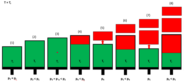
In a differential liberation test, a crude oil sample (green) is introduced into the cell at the initial reservoir pressure and temperature (Step 1 in Figure 3.07). The volume of the cell is then increased by extending the piston outward (Step 2), and the pressure and volume are recorded. At Step 2, the pressure in the cell will be less that the original pressure due to the expansion of the crude oil. This process is continued for several pressure steps until the first bubble of gas (red) is observed through a window in the cell (Step 3). This pressure is the bubble-point pressure of the crude oil. Up until the bubble-point pressure is reached, all measurements have been single-phase (liquid hydrocarbon) measurements.
After the bubble-point pressure has been reached, the volume is increased further until a significant volume of free gas has developed (Step 4). At this point, the pressure and the oil and gas volumes in the cell are measured. The gas is then expelled from the piston under isobaric (constant pressure) conditions by reducing the piston volume and allowing the gas to escape through a valve in the system (Step 5). This process is then repeated until the desired final pressure is reached (Step 8). The pressure, liquid volume, and gas volume are then used in the calculation of the appropriate properties for black oils.
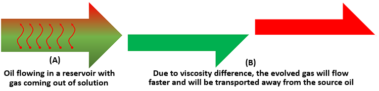
What is the differential liberation test trying to model? In the reservoir, as gas comes out of solution, it typically has a much lower viscosity than the oil phase. Consequently, as gas evolves from the oil, this difference in the viscosity allows the gas to move faster than the oil and to separate from the source oil from which it evolved. This is illustrated in Figure 3.08. In addition, due to the density differences between oil and gas phases, gravity will also act to separate the two phases. It is the properties of the separated phases that we are most interested in, as these are more representative of the processes occurring in the reservoir.
API Gravity of the Crude Oil, °API
In the oil and gas industry, crude oils are characterized by the API gravity (American Petroleum Institute gravity) of the oil. The units of the API gravity are degrees, °API (read as degrees API). The API gravity is defined as:
Where:
- ϒo is the specific gravity of the crude oil at 60 °F, dimensionless
- °API is the API gravity, degrees API
The API gravity scale acts as an inverse relationship to density (and specific gravity), that is, as density increases, the API gravity decreases. Crude oils are often graded by their API gravity:
- Light crude oil: °API > 31.5°
- Intermediate crude oil: 22.1° ≤ °API ≤ 31.5°
- Heavy crude oil: °API < 22.1o
Molecular Weight of the Crude Oil, MWo
Samples of the crude oil taken during the differential liberation test can be extracted from the PVT cell, and the compositions of the crude oil samples can be measured as functions of pressure. If the mole fractions, xi, of all components are measured from an oil sample (any sample, not just a sample from a differential liberation test), then the molecular weight in lbs/lbs-mole of the oil sample, MWo, can be calculated from:
If laboratory data are unavailable, then the Cragoe[7] correlation can be used to estimate the molecular weight:
Where:
- MWo is the molecular weight of the crude oil, lb/lb-mole
- °API is the API gravity, degrees API
Bubble-Point Pressure of the Crude Oil, pb
As already discussed, the bubble-point pressure is the pressure that first bubble of gas evolves from an undersaturated crude oil during pressure reduction. The laboratory method for calculating the bubble-point pressure, pb, of a crude oil was discussed earlier in the context of the differential liberation test. Other PVT tests, such as the Constant Composition Expansion Test, can be used to determine the bubble-point pressure of the crude oil. The constant composition expansion test is similar to the differential liberation test, however, the evolved gas is not expelled from the PVT cell during the test. For all measurements made up to and including the bubble-point pressure, the constant composition expansion test and the differential liberation test give identical results.
When measured data are not available, Standing’s correlation[8] can be used to estimate the bubble-point pressure:
with
Where:
- Rso is the solution gas-oil ratio of the crude oil, SCF/STB (to be discussed)
- ϒg is the gas gravity (MWg/MWair), dimensionless (to be discussed)
- T is the temperature, °F
- °API is the API gravity, degrees API
Solution Gas-Oil Ratio, Rso
As we have discussed, most crude oils (possibly excluding some extremely heavy crude oils: °API ≈ 10°) contain Dissolved Gas. This dissolved natural gas consists mostly of the low-end molecular weight hydrocarbons (methane, ethane, propane, and butane) and some inorganic impurities (nitrogen, carbon-dioxide, hydrogen-sulfide, etc.). The volume of this dissolved gas is quantified by the Solution Gas-Oil Ratio, Rso (sometimes simply referred to as Rs). The solution gas-oil ratio is defined as the volume of gas, measured is SCF or MSCF, in solution in 1.0 STB of crude oil. As such, it has the units of SCF/STB or MSCF/STB. A typical plot of Rso is illustrated in Figure 3.09.
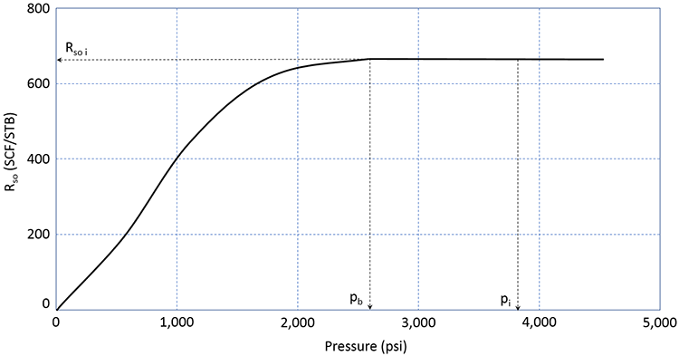
In this figure, we can see that the reservoir is an undersaturated oil reservoir. The initial reservoir pressure, pi, is greater than the bubble-point pressure. If this reservoir were to undergo pressure depletion from oil production, then the average reservoir pressure would decline over time, and the pressure would eventually reach the bubble-point pressure. During this time period, the volume of gas in solution in the crude oil remains constant at the initial value of Rso i.
Once the reservoir pressure reaches the bubble-point pressure, pb, gas begins to come out of solution. As the gas comes out of solution and evolves into Free Gas, the volume of gas remaining in solution, Rso, must decrease. This is the behavior observed in Figure 3.09. The volume of free gas liberated from the original stock tank barrel can be calculated as (Rso i – Rso) in SCF/STB or MSCF/STB.
The laboratory procedure for determining the solution gas-oil ratio was discussed in terms of the differential liberation test. The Rso values are calculated by summing the appropriate gas volumes obtained during the differential test and dividing by the final oil volume. When this is done, all volumes need to be corrected back to the reference volumes of STB and SCF to get to the appropriate Rso curve.
When laboratory derived Rso data are unavailable, then Equation 3.41 and Equation 3.42 can be used to estimate the solution gas-oil ratio. This is done by placing an assumed pressure into Equation 3.42 and using Equation 3.41 to calculate the pressure associated with that assumed Rso value (not the bubble-point pressure as explicitly written in the equation).
Oil Formation Volume Factor, Bo
The Oil Formation Volume Factor, Bo, is comparable to the water formation volume factor. It relates volume of 1.0 STB of crude oil at stock tank conditions, pST and TST, to its volume at reservoir conditions, pr and Tr. A typical plot of Bo is illustrated in Figure 3.10.
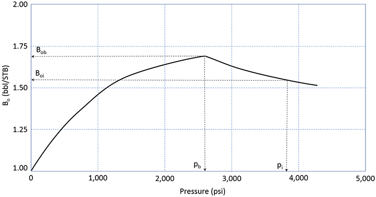
This figure shows the formation volume factor of the crude oil for the same reservoir as that shown in Figure 3.09 (identical pi and pb). As the pressure depletes from the initial pressure to the bubble-point pressure, the formation volume factor increases. This is indicative of the crude oil expanding (remember, the formation volume factor is based on 1.0 STB of oil – when the FVF increases, it is because the volume in reservoir barrels, bbl, of that STB is getting larger). This is the typical behavior that would be expected by a slightly compressible fluid - as confining pressure is reduced, we would expect that the volume would expand.
When the reservoir pressure reaches the bubble-point pressure, the formation volume factor begins to decrease. This is indicative of the crude oil shrinking. This is the opposite of the expected behavior of a slightly compressible fluid. This implies that as confining pressure is reduced the volume of the crude oil gets smaller. The reason for this behavior is that the crude oil is composed of the liquid hydrocarbon and the gas dissolved in it. As the gas comes out of solution, the crude oil loses the volume occupied by the solution gas.
Oil FVF above the Bubble-Point Pressure Pressure, p > pb
Because the formation volume factor of crude oil behaves differently above and below the bubble-point pressure, we must use correlations that show the proper trends. Since the crude oil behaves as a typical slightly compressible fluid above the bubble-point pressure, we can use the definition of compressibility, Equation 3.32, above the bubble-point pressure:
and
Where, for crude oils, we use pb as the reference pressure.
Oil FVF below the Bubble-Point Pressure, p < pb
Below the bubble-point pressure, we can use Standing’s correlation[8] to estimate the oil phase formation volume factor:
with
Where:
- Bo is the oil formation volume factor, bbl/STB
- Rso is the solution gas-oil ratio of the crude oil, SCF/STB
- ϒg is the gas gravity (MWg/MWair), dimensionless (to be discussed)
- ϒo is the oil specific gravity (ρo/ρw), dimensionless
- T is the temperature, °F
These equations are valid below and up to and including the bubble-point pressure. Therefore, we can use these equations to generate Bob for Equation 3.43b if it is unavailable from laboratory measurements.
Oil Phase Compressibility above the Bubble-Point Pressure, p > pb
As discussed, above the bubble-point pressure, crude oil acts like a slightly compressible fluid. One correlation for oil phase compressibility, co, above the bubble-point pressure from Vazquez and Beggs[9] is:
Where:
- co is the oil compressibility, 1/psi
- Rso is the solution gas-oil ratio of the crude oil (for p > pb; Rso = Rso i), SCF/STB
- T is the temperature, °F
- ϒg is the gas gravity (MWg/MWair), dimensionless (to be discussed)
- °API is the API gravity, degrees API
- p is the pressure, psi
Oil Phase Compressibility below the Bubble-Point Pressure, p ≤ pb.
Crude oil above the bubble-point pressure can contain large amounts of dissolved solution gas (high values of Rso). At higher Rso values, the crude oil has higher compressibility values due to the solution gas. At pressures below the bubble-point pressure, gas comes out of solution and the compressibility values begin to get smaller as the crude oil tends to behave more and more like a Dead Oil (dead oil is gas free oil; while crude oil with dissolved gas is often referred to as Live Oil). One common correlation for oil phase compressibility, co, below the bubble-point pressure from McCain, Rollins, and Villena[10] is:
Equation 3.46b
Where:
- co is the oil compressibility, 1/psi
- p is the pressure, psi
- T is the temperature, °F
- °API is the API gravity, degrees API
- Rso b is the solution gas-oil ratio of the crude oil at pb (Rso b = Rso i), SCF/STB
Oil Phase Density above the Bubble-Point Pressure, p > pb
One the values of pb, Rso, ϒg, Bo, and co are determined (either by laboratory measurements or by correlations), the oil phase density itself is specified (there are degrees of freedom remaining for ρo). As we discussed earlier, above the bubble-point pressure, crude oil behaves like a slightly compressible fluid. As such, we can use the definition of compressibility based on density:
Now, if we assume 1.0 STB of oil, at reservoir conditions, then we have:
and
Substituting Equation 3.48 into Equation 3.47 results in:
After integration of Equation 3.49 we have:
Oil Phase Density below the Bubble-Point Pressure, p ≤ pb
Below the bubble-point pressure, the crude oil loses mass (mass of the liberated gas), so we must account for the mass of the liquid oil and the mass of the gas remaining in solution when estimating the oil density below the bubble-point pressure. We can do this with a simple material balance. Below (and up to) the bubble-point pressure, the density of the crude oil can be calculated by dividing the total mass of the oil plus dissolved gas by the total volume. In terms of the properties discussed so far, we have:
Where:
- ρo is the oil density, lb/ft3
- ρo ST is the density of the dead oil (gas free oil) at stock tank conditions, lb/ft3
- ϒg is the gas gravity (MWg/MWair), dimensionless (to be discussed)
- Rso is the solution gas-oil ratio of the crude oil at pr and Tr, SCF/STB
- Bo is the oil phase formation volume factor at pr and Tr, bbl/STB
Note that we can use the properties in at the bubble-point pressure, Rso i and Bob, in Equation 3.51 to obtain ρob for input into Equation 3.50.
Oil Phase Viscosity above the Bubble-Point Pressure, p > pb
The viscosity of a crude oil is also impacted by the amount of gas in solution. The typical viscosity behavior of crude oil is shown in Figure 3.11.
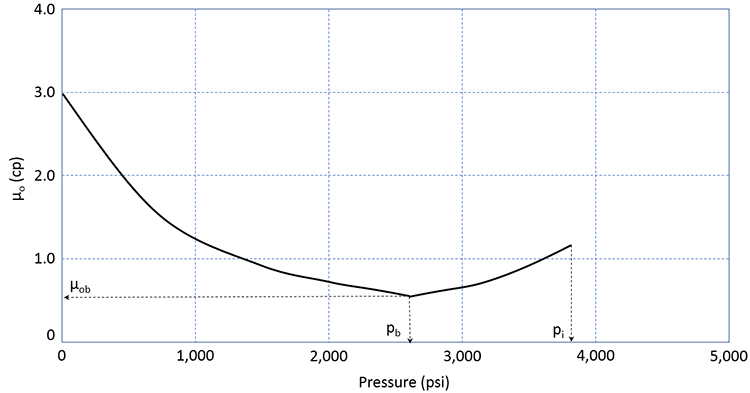
Oil Phase Viscosity below the Bubble-Point Pressure, p ≤ pb
The estimation of the oil viscosity below the bubble-point pressure is a two-step process. In the first step, the dead oil (gas free) viscosity is calculated and in the second step the live oil (oil with solution gas) viscosity is calculated. The dead oil viscosity at reservoir temperature can be calculate by[11]:
The second step is to calculate the live oil viscosity with the dissolved gas:
with
and
Where:
- A and B are correlation parameters
- μoD is the dead oil at Tr, cp
- °API is the API gravity, degrees API
- T is the temperature, °F
- Rso is the solution gas-oil ratio of the crude oil at pr and Tr, SCF/STB
Oil Phase Viscosity above the Bubble-Point Pressure, p > pb
The oil viscosity above the bubble-point pressure can found by calculating the viscosity at the bubble-point pressure, μob and Rso i, and adjusting it to higher pressures[11]:
with
Where:
- C is a correlation parameter
- μob is the live oil viscosity at pb and Tr, cp
- p is the pressure of interest, psi
- pb is the bubble-point pressure, psi
[7] Cragoe, C.S.: “Thermodynamic Properties of Petroleum Products,” U.S. Dept. of Commerce, Washington, DC (1929) 97.
[8] Standing, M.B.: Volumetric and Phase Behavior of Oil Field Hydrocarbon Systems, SPE, Richardson, TX (1977) 124.
[9] Vazquez, M. and Beggs, H.D.: "Correlations for Fluid Physical Property Prediction," JPT (June 1980) 968-70.
[10] McCain, W.D. Jr., Rollins, J.B., and Villena, A.J.: "The Coefficient of Isothermal Compressibility of Black Oils at Pressures Below the Bubblepoint," SPEFE (Sept. 1988) 659-62; Trans., AIME, 285. 10.
[11] W.D. McCain .Jr. “Reservoir·Fluid Property Correlations-State of the Art,” SPE Reservoir Engineering, (May 1991) p. 266.
3.3.3: Natural Gas Properties
For natural gases we are also most interested in the Gas Formation Volume Factor, Bg, and the Gas Viscosity, μg, as these properties strongly influence gas storage (and accumulation) and gas flow. For most reservoir engineering calculations, the gas formation volume factor (and Gas Compressibility, cg, and Gas Density, ρg) can be determined from the Real Gas Law, Equation 3.27:
Where:
- p is the pressure of interest, psi
- V is the volume, ft3
- Z is the oil super-compressibility factor, dimensionless
- R is the gas constant, (psi ft3) / (lb-moles °R)
- T is temperature, °R (°R = °F + 460.67)
Gas Super-Compressibility Factor, Z
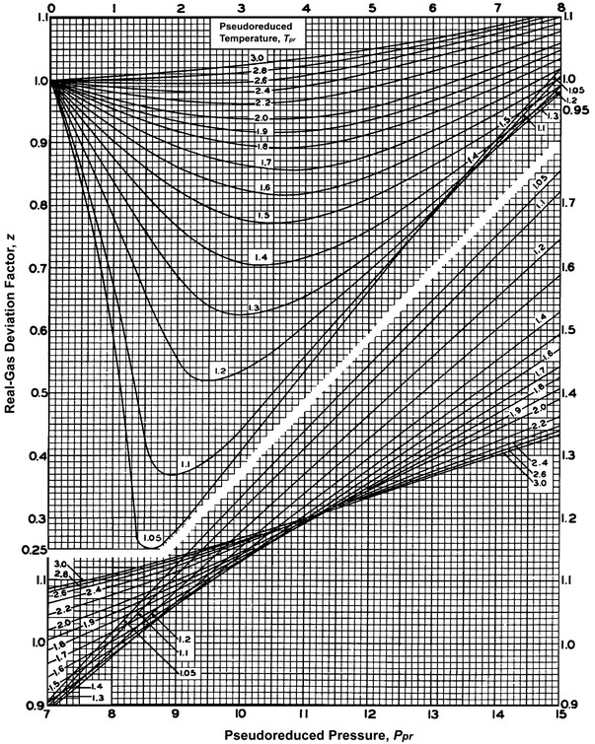
The gas supercompresibility factor, Z (or Z-Factor, or Real Gas Deviation Factor), is a function of pressure and temperature that corrects the Ideal Gas Law for high pressure and high temperature conditions. In the oil and gas industry, the z-factor correlation for hydrocarbon gases that is universally accepted in the Standing-Katz Correlation[12]. This correlation is shown graphically in Figure 3.12.
As illustrated in Figure 3.12 The Standing-Katz Correlation correlates the z-factor to the Pseudo-Reduced Pressure, ppr, and Pseudo-Reduced Temperature, Tpr. The pseudo-reduced properties are defined by:
and
Where:
- p is the pressure of interest, psi
- ppc is the pseudo-critical pressure, psi
- T is temperature of interest, °R
- Tpc is pseudo-critical temperature, °R
All of these properties are called pseudo-properties because the pseudo-critical pressure and pseudo-critical temperature are not the true, measured critical properties, but are calculated properties:
and
with
Where:
- ppc is the pseudo-critical pressure, psi
- Tpc is the pseudo-critical temperature, °R
- ϒg is the gas gravity (MWg/MWair), dimensionless
- MWg is the molecular weight of the gas, lb/lb-mole
- MWair is the molecular weight of air, lb/lb-mole (28.97 lb/lb-mole)
In cases where significant concentrations of inorganic impurities, CO2 and H2S are present, then corrections to Equation 3.61 and Equation 3.61 are required:
and
with
Where:
- ppc corrected is the corrected pseudo-critical pressure, psi
- ppc Eq. 3.61 is the pseudo-critical pressure from Equation 3.61, psi
- Tpc corrected is the corrected pseudo-critical temperature, °R
- Tpc Eq. 3.60 is the corrected pseudo-critical from Equation 3.60, °R
- ϵcorrection is the correction for CO2 and H2S, °R
- yCO2 is the mole fraction of CO2 in the gas phase, fraction
- yH2S is the mole fraction of H2S in the gas phase, fraction
The Standing-Katz[12] correlation has also been mathematically curve fit[13]. The equation for z-factor then becomes:
with
It should be noted that the solution of this equation for the z-factor requires an iteration procedure. This is because the z-factor appears both on the left-hand side of Equation 3.66 and the right-hand side of the equation through the pseudo-reduced density, ρpr. Typically, this is solved with a Newton-Raphson iteration procedure which is beyond the scope of this class. For our purposes, if supercompressibility factors are required, we can simply read the chart to obtain them.
Real Gas Formation Volume Factor, Bg
The Formation Volume Factor, Bg, of a real gas, like its oil phase analog, is used to convert one standard cubic foot, SCF, of gas at reference conditions to its volume at reservoir conditions. For natural gases, in the U.S. domestic oil and gas industry, we use the standard conditions of pSC = 14.7 psi and 60 °F. The gas formation volume factor for a real gas can be calculated directly from the Real Gas Law once we have an estimate of the super-compressibility factor. If we assume one lb-mole of natural gas, then the volume that it would occupy at standard conditions would be (assuming ZSC = 1.0 at standard conditions – a very good assumption):
At reservoir conditions, that same lb-mole would occupy a volume of:
Now, the gas phase formation volume factor we can define as:
There are times when we would like to consider the volume of gas in reservoir barrels, bbl. This is because we have used reservoir barrels as the units for the liquid (oil and water) volumes, and we would like to determine the volume occupied by the gas and liquids combined. We can convert the units of Equation 3.68a by applying the unit conversion constant of 1 bbl = 5.615 ft3:
Where:
- Bg is the gas formation volume factor, ft3/SCF (Equation 3.68a) or bbl/SCF (Equation 3.68b)
- Z is the supercompressibility factor at reservoir conditions, pr and Tr, dimensionless
- Tr is the reservoir temperature, °R
- TSC is the reference (standard) temperature (520 °R in U.S. domestic industry), °R
- pr is the reservoir pressure, psi
- pSC is the reference (standard) pressure (14.7 psi in the U.S. domestic industry), psi
Real Gas Compressibility, cg
The isothermal compressibility of a real gas can also be determined directly from the Real Gas Law. Starting with the definition of isothermal compressibility:
Substituting the Real Gas Law, Equation 3.27, into Equation 3.69:
or
The derivative, , can be calculated by differentiating Equation 3.66 and Equation 3.67 with respect to pressure.
Real Gas Density, ρg
The density of a real gas can also be determined directly from the Real Gas Law. Starting with the Real Gas Law:
Now the number of moles is equal to a mass divided by the molecular weight, n = m / MWg. Substituting into the Real Gas Law:
Now from the definition of gas density and the substitution of the Real Gas Law:
Where:
- ρg is the gas density, lb/ft3
- p is the pressure of interest, psi
- MWg is the molecular weight of the gas, lb/lb-mole
- Z is the supercompressibility factor at reservoir conditions, pr and Tr, dimensionless
- R is the Gas Constant, 10.73 ft3 psi / °R lb-mole
- T is the temperature of interest, °R
Real Gas Specific Gravity, γg
The specific gravity of a real gas can also be determined directly from the Real Gas Law. For gases, the specific gravity is defined as the ratio of the density of the gas to the density of air at standard conditions. Dividing Equation 3.71 written for a gas by Equation 3.71 written for air at standard conditions (Z = 1.0) results in:
Now, the molecular weight of gas is 28.87 lb/lb-mole:
Real Gas Viscosity, μg.
The viscosity of natural gases can be determined by the correlation of Lee, Gonzalez, and Eakin[14]:
with
Where:
- μg is the gas viscosity, cp
- K, X, and Y are correlation coefficients
- ρg is the gas density at the pressure and temperature of interest, gm/cc
- MWg is the molecular weight of the gas, lb/lb-mole
- T is the temperature of interest, °R
[12] Standing, M.B. and Katz, D.L.: "Density of Natural Gases," Trans., AIME (1942) 146, 140-49.
[13] Dranchuk, P.M. and Abou-Kassem, J.H.: "Calculations of z-Factors for Natural Gases Using Equations of State," J. Cdn. Pet. Tech. (July-Sept. 1975) 34-36.
[14] Lee, A.L., Gonzalez, M.H., and Eakin, B.E.: "The Viscosity of Natural Gases," JPT (Aug. 1966) 997-1000; Trans., AIME (1966) 234.
3.4: Reservoir Rock - Fluid Interaction Properties
To this point in the lesson, we have discussed Rock Properties and Fluid Properties, but we must also discuss how the rock and different fluids interact. In other words, how does the rock interact with the fluids and how do the various fluids interact with each other? At the pore and capillary scales, these interactions occur through the various attractive and repulsive forces acting on each component in the system (rock and fluids). These pore-scale forces include capillary forces, surface tensions, interfacial tensions, van der Waal forces, etc. While these topics are interesting in their own right, as engineers, we are interested in how these pore and capillary scale forces manifest themselves at a much larger macro-scale.
Phase Saturations, So, Sg, and Sw
To start the discussion about rock-fluid interaction properties, we must first define the phase saturations, So, Sg, and Sw, in the reservoir. The phase saturation is defined as the fraction of the pore volume occupied by a particular phase. For example, if the pore-volume of a porous medium by 65 percent oil, 25 percent gas, and 10 percent water, then the phase saturations would be:
- So = 0.65
- Sg = 0.25
- Sw = 0.10
Thus, if we had a core sample of rock with a bulk volume, Vb = 200.0 cc, an effective porosity, ϕ = 0.22, and the phase saturations listed above, then the core sample would contain:
- Vo=So Vp=SoϕVb = (0.65)(0.22)(200.0 cc) = 28.6 cc of oil
- Vg=Sg Vp=SgϕVb = (0.25)(0.22)(200.0 cc) = 11.0 cc of gas
- Vw=Sw Vp=SwϕVb = (0.10)(0.22)(200.0 cc) = 4.4 cc of water
where Vo, Vg, and Vw are the volumes of oil, gas, and water, respectively, in the core sample. By definition, the phase saturations must always sum to 1.0:
This relationship is known as the Saturation Constraint.
Capillary Pressure, pcow and pcgo
It has been observed that when two or more immiscible fluids occupy the pore-volume and capillaries of a porous medium, the pressures of the different phases are not equal, but are different from each other. This macro-scale phenomenon, known as capillary pressure, is due to interactions of the surface and interfacial tensions of the rock and fluids in the confined dimensions of the rock pores and capillaries. A force balance on the surface and interfacial tensions require that the pressures of the various phases are different. At the macro-scale, this phenomenon is quantified with the Capillary Pressure Relationships:
and
As shown in Equation 3.77 and Equation 3.78, the capillary pressure is the difference between the two phase pressures and is a function of the phase saturations. As written, these equations assume that the reservoir rock is Water Wetting Surface (the surface of the rock preferentially favors contact with the water phase). If we were to write these equations for an Oil Wetting Surface (the surface of the rock preferentially favors contact with the oil phase), then we would have:
and
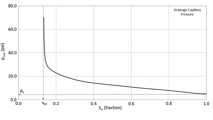
We will not go into the details of Wettability, Water Wetting Surfaces, or Oil Wetting Surfaces; however, water wet reservoirs are the more common for petroleum rocks, and we will focus on them (Equation 3.77 and Equation 3.78). Please note that while water wetting rocks are the more common for reservoir rock lithologies, there are many examples of oil wet rocks in the petroleum literature. Figure 3.13 shows a typical drainage capillary pressure relationship for a water wet rock.
In Figure 3.13, the solid line is the drainage capillary pressure curve for a wetting phase (in our case, water in a water-wet rock). The capillary pressure, pe, is the Entry Pressure which is the pressure that is required to force a non-wetting phase (in our case, oil in a water-wet rock). The entry pressure is the pressure that is required to force the first drop of oil into the water-wet rock. Remember, the term “water-wet” implies that the rock has a preference to stay in contact with water. The entry pressure is the pressure required to overcome this preference. At some value of water saturation, the capillary pressure measurements begin to go asymptotic to the vertical. This water saturation, Swir, is the Irreducible Water Saturation and represents the minimum water saturation that the reservoir rock can reach in the presence of an oil phase. As indicated in this figure, irreducible water saturation is caused by capillary forces acting on the oil, water, and rock components of the system.
In this figure, the term “Drainage Capillary Pressure” appears; this refers to the manner in which the data were measured. There are two ways that we can measure capillary pressure. We could first fill the core sample with the wetting phase (in our case, water) and measure the capillary pressure by increasing the saturation of the non-wetting phase (in our case oil). This is identical to decreasing the saturation of the wetting-phase. This process, where the wetting phase saturation is decreased, is referred to as a Drainage Process and represents processes where the wetting phase is allowed to “drain” from the rock.
Alternatively, we could have first filled the core sample with the non-wetting phase (in our case, oil) and measured the capillary pressure by increasing the saturation of the wetting phase (in our case, water). This process, where the wetting phase saturation is increased, is referred to as an Imbibition Process and represents processes where the wetting phase is allowed to “imbibe” into the core. Both processes, drainage processes and imbibition processes, occur in oil and gas reservoirs.
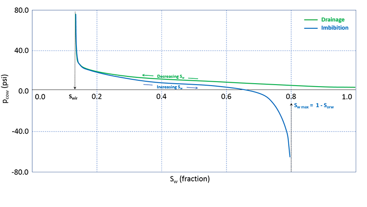
It turns out that when you conduct the experiment using these two processes, you get different results. When this phenomenon occurs (measurements are dependent on the saturation history – increasing or decreasing wetting phase saturation), it is referred to as Hysteresis. Typical results for oil-water drainage and imbibition capillary pressure measurements including the impact of hysteresis are shown in Figure 3.14.
In Figure 3.14, we see that as we increase the saturation during an imbibition measurement cycle, the water saturation reaches an asymptotic maximum value, Sw max (or, 1 - Sorw). This trapped oil saturation, Sorw, is called the Residual Oil Saturation to Water and is the result of capillary forces occurring in the reservoir rock. We will discuss these end-point saturations, Swir and Sorw, in more detail when we discuss relative permeabilities.
While both drainage processes and imbibition processes occur in the reservoir, the topic of hysteresis is beyond the scope of this course. For this course, we will focus on the drainage capillary pressure of water wet reservoirs.
In the laboratory, capillary pressures are measured using Special Core Analysis (also known as SCAL) methods and must be specifically requested from the core laboratory. The drainage capillary pressure curves (Figure 3.13 and green curve in Figure 3.14) can be estimated from the Brooks-Corey Model[15]:
Where:
- pcow is the oil-water capillary pressure, psi
- λ is the pore-size distribution, dimensionless
- po and pw are the pressures of the oil phase and water phase, respectively, psi
- pe is the entry pressure, psi
- Sw is the water (wetting) phase saturation, fraction
- Swir is the irreducible water saturation, fraction
In the Brooks-Corey Model[15], λ, Swir, and pe can be obtained from the capillary pressure data. In addition, Swir can be obtained from open-hole well logs or by relative permeability data.
Relative Permeability, krow and krw
We have already discussed Darcy’s Law in the context of single-phase flow and absolute permeability. Darcy’s Law, Equation 3.24, was written earlier as:
Where qf is the volumetric flow rate in bbl/day, and all of the properties used in Equation 3.24 were discussed earlier. Note that we can convert the units of flow rate in Darcy’s Law from bbl/day to STB/day by the inclusion of the formation volume factor of the flowing fluid, Bf:
One of the assumptions listed with these versions of Darcy’s Law was that the flowing fluid is an incompressible, homogeneous, Newtonian fluid that fully saturates (single-phase) the porous medium. As we have already seen, the flow of fluids in real petroleum reservoirs is typically up to three-phase flow, and in some rare instances, may be as high as four-phase flow.
For multi-phase flow, we can rewrite Equation 3.82 for each of the phases present, regardless of whether the fluids are mobile or are stationary (we only care about their presence). Assuming three phases; oil, water, and gas, we have:
and
Note that we have assigned a phase designation to both the pressure, pf, and the permeability, kf. As discussed earlier, due to the capillary pressures, each of the phases present in the reservoir may have a different pressure, and consequently, we must distinguish between pressures (and pressure gradients) that are specific to each phase.
When we write a permeability value that is specific to an individual phase, kf, that permeability is referred to as the Effective Permeability to that phase. Therefore, in Equation 3.83, we have the effective permeability to oil, the effective permeability to water, and the effective permeability to gas (ko, kw, and kg, respectively).
The effective permeability is defined as the permeability to a specific phase in the presence of one or more other phases. These effective permeabilities, kf, are related to the absolute permeability, k, appearing in Equation 3.24 and Equation 3.82 through the Relative Permeability Relationships:
and
Where:
- kro, krw, and krg are the relative permeabilities to oil, water and gas, respectively, fraction
- k is absolute permeability (permeability for single-phase flow: Equation 3.24 and Equation 3.82), md
Substituting Equation 3.84 into these into Equation 3.83:
and
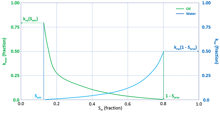
Relative permeabilities are functions of the phase saturations. A typical set of oil-water relative permeability curves is shown in Figure 3.15.
In Figure 3.15, the water saturation is plotted on the x-axis. The most important features that can be seen in this figure are the trends of the relative permeability curves. As the water saturation increase, the relative permeability to oil decreases while the relative permeability to water increases. This is because as the water saturation increases, fewer pathways become available for oil to flow while more pathways become available for water to flow.
In this figure, the parameters of irreducible water saturation, Swir, and residual oil saturation to water, Sorw, are identical to the values discussed earlier in the section on capillary pressure curves and shown in Figure 3.14. The water saturation range, Swir ≤ Sw ≤ 1 – Sorw, represents the range in which both the oil and water are mobile. Note that outside of this range, one of the relative permeability values is equal to zero, from Equation 3.85 a zero value of relative permeability implies that the flow rate will be zero.
On this plot, we can see that the maximum water saturation, Sw max = 1 – Sorw. We use this terminology because, as stated, the x-axis is the water saturation; while Sorw is an oil saturation. In other words, from Figure 3.15 we can see that Sorw is approximately 0.2, while due to the saturation constraint, ∑f=o,wSf = 1, Sw max must be 0.8.
For a two-phase, oil-gas system we have a somewhat similar set of relative permeability curves as with the two-phase, oil-water system. Figure 3.16 shows a typical set of gas-oil relative permeability curves.
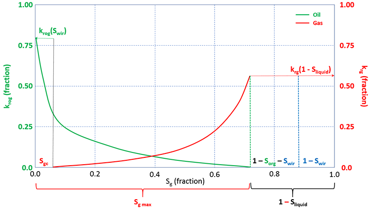
In the gas-oil relative permeability curves, the gas saturation, Sg, is plotted on the x-axis. There are several important differences between the oil-gas system and the oil-water system that must be further discussed. One difference is the critical gas saturation, Sgc. The critical gas saturation is similar to Swir for water, in that it represents the value at which gas will begin to flow in situations the gas saturation is increasing (or, conversely, the saturation at which gas will stop flowing in situations the gas saturation is decreasing). We can also see oil is present and is mobile below Sgc (it has finite values below Sgc). This is because of the dissolved gas in the oil phase. As gas comes out of solution from a mobile oil phase, the gas saturation needs to build up to Sgc before it can begin to flow. While this is occurring, the oil phase remains mobile. Therefore, for gas-oil systems, oil is mobile in the range 0 ≤ Sg ≤ 1 – Sorg – Swir, and gas is mobile in the range Sgc ≤ Sg ≤ 1 – Sorg – Swir.
A second difference between the oil-water curves and the gas-oil curves is the use of the term krow in Figure 3.15 and the term krog in Figure 3.16. This is because the relative permeabilities to oil are different when measured in an oil-water system and in a gas-oil system. The is also true for the residual oil saturations, Sorw and Sorg. These differences are due to the differences in the surface tensions and resulting capillary forces between oil and water and between gas and oil.
A third difference is due to the irreducible water saturation, Swir. As we have already discussed, the irreducible water saturation is the lowest water saturation in the reservoir. Since all real oil and gas reservoirs contain water, the initial water saturation in these reservoirs, Swi, must be at least equal to the irreducible water saturation, Swir, or greater: Swi ≥ Swir. Therefore, to get representative laboratory measurements or calculations from correlations, we must include Swir in the analyses. Therefore, when we take laboratory measurements for gas-oil curves, we take them in the presence of an immobile, irreducible water saturation. Also note the application of the saturation constraint for the liquid (oil and water) saturations.
Relative permeability measurements also require special laboratory techniques and must be requested as a part of Special Core Analysis procedures when ordering tests from a core laboratory. There are two general approaches for laboratory measurements of relative permeability, the Unsteady State Method and the Steady State Method. Of the two methods, the Steady State Method (also known as the Penn State Method) is the more accurate laboratory procedure; however, it takes more time (and money) to perform these tests.
When laboratory data are not available, then the relative permeabilities can be calculated using a Power Law Model.
For oil-water curves, we have:
and
While for gas-oil systems we have:
and
Where:
- krow is the relative permeability to oil measured in an oil-water system, fraction
- krw is the relative permeability to water measured in an oil-water system, fraction
- krog is the relative permeability to oil measured in a gas-oil system in the presence of an irreducible water saturation, fraction
- krg is the relative permeability to gas measured in a gas-oil system in the presence of an irreducible water saturation, fraction
- krow(Swir) is the relative permeability to oil at the irreducible water saturation measured in an oil-water system, fraction
- krw(1 – Sorw) is the relative permeability to water at the maximum water saturation, measured in an oil-water system, fraction
- krog(Swir) is the relative permeability to oil at the irreducible water saturation measured in a gas-oil system in the presence of an irreducible water saturation, fraction
- krg(1 – Sliquid) is the relative permeability to gas at the maximum gas saturation, 1 – Sorg – Swir, in a gas-oil system in the presence of an irreducible water saturation, fraction
- So, Sw, and Sg are the oil, water, and gas saturations, respectively, fraction
- Swir is the irreducible water saturations, fraction
- Sorw is the residual oil saturation to a water displacement
- Sorg is the residual oil saturation to a gas displacement in a gas-oil system in the presence of an irreducible water saturation, fraction
- Sgc is the critical gas saturation where gas begins to flow in a gas-oil system in the presence of an irreducible water saturation, fraction
- now and nw are oil and water exponents, respectively, in an oil-water system (these exponents are referred to as Corey Exponents), dimensionless
- nog and ng are oil and gas exponents, respectively, in a gas-oil system in the presence of an irreducible water saturation (these exponents are also referred to as Corey Exponents), dimensionless
Most of these values can be seen in Figure 3.15 and Figure 3.16. Note that all of the groups in the parenthesis in Equation 3.86 through Equation 3.87 go from 0.0 to 1.0 in their respective mobile saturation ranges. These groups are often referred to as Normalized Saturations.
[15] Brooks, R.H. and Corey, A.T. 1964. Hydraulic Properties of Porous Media. Hydrology Paper No. 3, Colorado State University, Fort Collins, Colorado, 22–27.
3.5: Key Learnings
In this lesson, we discussed the following topics:
- The properties of interest to petroleum engineers are divided into three categories:
- Rock properties
- Fluid properties
- Rock-Fluid interaction properties
- These properties are most commonly used to improve our understanding of:
- Storage of oil, water, and gas in a petroleum reservoir
- Transport (movement) of oil, water, and gas in the reservoir
- The rock properties that we discussed included:
- Porosity (ability of a rock to store fluids)
- Compressibility (property of the rock that governs how volumes behave with changes in pressure)
- Permeability (ability of a rock to transmit fluids)
- Common methods used to determine porosity are:
- Laboratory measurements
- Grain determination by immersion
- Grain determination by Boyle’s Law
- Washburn-Bunting (mercury injection)
- Summation of fluids
- Well logs (field measurements):
- Sonic log
- Density log
- Neutron log
- Laboratory measurements
- Common methods used to determine permeability are:
- Laboratory measurements: Core Floods
- Field measurements:
- Well tests (or pressure transient analysis)
- Permeability-porosity cross-plots
- Fluid Properties:
- Formation volume factor: oil, gas, and water property that describes the reservoir volume occupied by one STB of liquid or one SCF of gas
- Compressibility: oil, gas, and water property that describes the change in volume with a change in pressure
- Viscosity: oil, gas, and water property that describes the ease with which a fluid can flow through a porous medium
- Density: oil, gas, and water property that quantifies the weight of a unit volume of fluid
- Specific gravity: oil, gas, and water property that normalizes the density to the density of a standard fluid – water for liquids and air for gases
- Bubble-point pressure: oil property describing the pressure that the first bubble of gas evolves from the oil with reducing pressures
- Solution Gas-Oil Ratio: oil property describing the amount of gas (in SCF) dissolved in one STB of oil
- Gas super-compressibility or real gas deviation factor: gas property that describes the deviation of a real gas from the ideal gas law
- API Gravity: oil property related to specific gravity
- Molecular weight: oil, gas, and water property that quantifies the weight of one mole of fluid molecules
- These properties (excluding molecular weight and specific gravity) are, in general, pressure dependent properties
- Rock-fluid interaction properties
- Phase saturation: oil, gas, and water property describing the fraction of the pore-volume occupied by the phase
- Capillary pressure: oil-water and gas-oil property that describes the difference in the pressures between the paired pressures
- Effective permeability: oil, gas, and water property that describes the permeability to one phase in the presence of one or more other phases in the porous medium
- Relative permeability: oil, gas, and water property that is the ratio of the effective permeability to a phase divided by the absolute permeability of the porous medium
- These properties are, in general, saturation dependent properties
3.6: Summary and Final Tasks
Summary
In this lesson, we learned that the two most critical considerations in petroleum engineering in general, and reservoir engineering, in particular, are the ability of the reservoir rock to store fluids and the ability of the reservoir rock to transmit fluids. We then learned that the properties that govern these two considerations can be divided into three categories: rock, fluid, and rock-fluid interaction properties. We also saw how properties within these categories need to be integrated to make meaningful analyses of subsurface phenomenon. For example, the multiphase version of Darcy’s Law, Equation 3-85, contains rock properties (permeability), fluid properties (viscosity and formation volume factor), and rock-fluid interaction properties (capillary pressure and relative permeability).
In addition, we discussed the data sources (field, laboratory, or derive from correlations) of the required data. We saw that there were multiple sources of reservoir properties. For rock properties, we saw that laboratory (core) and field measurements could be used (for example, core experiments and well logs for porosity determination and core floods and well tests for permeability determination).
For fluid properties, we saw that laboratory measurements (PVT cell) and property correlations could be used. We also saw that most of the fluid properties are pressure dependent.
Finally, we discussed the rock-fluid interaction properties. We started this discussion with an introduction to phase saturations and continued to discuss capillary pressures and relative permeabilities. We saw that the rock-fluid interaction properties were dependent on the phase saturations.
Final Tasks
Complete all of the Lesson 3 tasks!
You have reached the end of Lesson 3! Double-check the to-do list on the Lesson 3 Overview page [4] to make sure you have completed all of the activities listed there before you begin Lesson 4.