Phase Diagrams, Part IV
Module Goals
Module Goal: To familiarize you with the basic concepts of Phase Diagrams as a means of representing thermodynamic data.
Module Objective: To familiarize you with the process of extracting quantitative compositional information from phase envelopes.
Effect of Composition on Phase Behavior
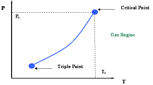
Let us try to reconcile the P-T graphs for the binary mixture with what we know from P-T graphs for single-component systems. At the end of the day, a mixture is formed by individual components which, when pure, act as presented in the P-T diagram shown in Fig. 3.1 [Module 3, repeated below]. We would, therefore, expect that the P-T diagram of each pure component will have some sort of influence on the P-T diagram of any mixture in which it is found.
In fact, it would be reasonable to think that as the presence of a given component A dominates over B, the P-T graph of that mixture (A+B) should get closer and closer to that of A as a pure component.
What this is telling us is that a new variable is coming into the picture: composition. So far we have not considered the ratio of component A to component B in the system. Now we are going to study how different ratios (compositions) will give different envelopes, i.e., different P-T behaviors.
Let us say that we have a mixture of components A (Methane, CH4) and B (Ethane, C2H6), where A is the more volatile of the two. It is clear that for the two pure components, we would have two boiling point curves for each component (A and B) as shown in Figure 5.1.
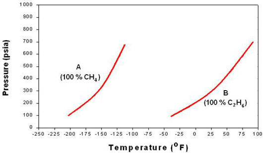
Please notice that the position of each of curve with respect to the other depends on its volatility. Since we are considering A to be the more volatile, it is expected to have higher vapor pressures at lower temperatures, thus, its curve is located towards the left. For B, the less volatile component, we have a boiling point curve with lower vapor pressures at higher temperatures. Hence, the boiling point curve of B is found towards the right at lower pressures.
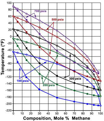
Now, if we mix A and B, the new phase envelope can be anywhere within curves A and B. This is shown in Figure 5.2, where the effect of composition on phase behavior of the binary mixture Methane/Ethane is illustrated.
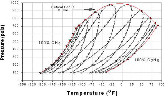
In Figure 5.2, each phase envelope represents a different composition or a particular composition between A and B (pure conditions). The phase envelopes are bounded by the pure-component vapor pressure curve for component A (Methane) on the left, that for component B (Ethane) on the right, and the critical locus (i.e., the curve connecting the critical points for the individual phase envelopes) on the top. Note that when one of the components is dominant, the curves are characteristic of relatively narrow-boiling systems, whereas the curves for which the components are present in comparable amounts constitute relatively wide-boiling systems.
Notice that the range of temperature of the critical point locus is bounded by the critical temperature of the pure components for binary mixtures. Therefore, no binary mixture has a critical temperature either below the lightest component’s critical temperature or above the heaviest component’s critical temperature. However, this is true only for critical temperatures; but not for critical pressures. A mixture’s critical pressure can be found to be higher than the critical pressures of both pure components — hence, we see a concave shape for the critical locus. In general, the more dissimilar the two substances, the farther the upward reach of the critical locus. When the substances making up the mixture are similar in molecular complexity, the shape of the critical locus flattens down.
Px and Tx Diagrams
In addition to considering variations with pressure, temperature, and volume, as we have done so far, it is also very constructive to consider variations with composition. Most literature on the subject calls these diagrams the “P-x” and “T-x” diagrams respectively. However, a word of caution is needed in order not to confuse the reader. Even though “x” stands for “composition” — in a general sense — here, we will see in the next section that it is also customary to use “x” to single out the composition of the liquid phase. In fact, when we are dealing with a mixture of liquid and vapor, it is customary to refer to the composition of the liquid phase as “xi” and use “yi” for the composition of the vapor phase. “xi” pertains to the amount of component in the liquid phase per mole of liquid phase, and “yi” pertains to the amount of component in the vapor phase per mole of vapor phase. However, when we talk about composition in general, we are really talking about the overall composition of the mixture, the one that identifies the amount of component per unit mole of mixture. It is more convenient to call this overall composition “zi”. If we do so, these series of diagram should be called “P-z” and “T-z” diagrams. This is a little awkward in terms of traditional usage; and hence, we call them “P-x” and “T-x” where “x” here refers to overall composition as opposed to liquid composition.
A P-x diagram for a binary system at constant temperature and a T-x diagram for a binary system at a constant pressure are displayed in Figures 5.3 and 5.4, respectively. The lines shown on the figures represent the bubble and dew point curves. Note that the end points represent the pure-component boiling points for substances A and B.
(Courtesy of ©LOMIC, INC)
In a P-x diagram (Figure 5.3), the bubble point and dew point curves bound the two-phase region at its top and its bottom, respectively. The single-phase liquid region is found at high pressures; the single-phase vapor region is found at low pressures. In the T-x diagram (Figure 5.4), this happens in the reverse order; vapor is found at high temperatures and liquid at low temperatures. Consequently, the bubble point and dew point curve are found at the bottom and the top of the two-phase region, respectively.
The Lever Rule
P-x and T-x diagrams are quite useful, in that information about the compositions and relative amounts of the two phases can be easily extracted. In fact, besides giving a qualitative picture of the phase behavior of fluid mixtures, phase diagrams can also give quantitative information pertaining to the amounts of each phase present, as well as the composition of each phase.
For the case of a binary mixture, this kind of information can be extracted from P-x or T-x diagrams. However, the difficulty of extracting such information increases with the number of components in the system.
At a given temperature or pressure in a T-x or P-x diagram (respectively), a horizontal line may be drawn through the two-phase region that will connect the composition of the liquid (xA) and vapor (yA) in equilibrium at such condition — that is, the bubble and dew points at the given temperature or pressure, respectively. If, at the given pressure and temperature, the overall composition of the system (zA) is found within these values (xA < zA < yA in the T-x diagram or yA < zA < xA in the P-x diagram), the system will be in a two-phase condition and the vapor fraction (αG) and liquid fraction (αL) can be determined by the lever rule:
(5.1a)
(5.1b)
Note that αL and αG are not independent of each other, since αL + αG = 1. Figure 5.5 illustrates how equations (5.1) can be realized graphically. This figure also helps us understand why these equations are called “the lever rule.” Sometimes it is also known as the “reverse arm rule,” because for the calculation of αL (liquid) you use the “arm” within the (yA-xA) segment closest to the vapor, and for the vapor calculation (αG) you use the “arm” closest to the liquid.
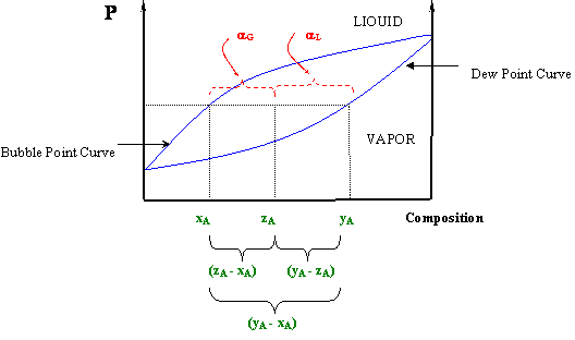
At this point you will see clearly why we needed to make a clear distinction among “xi” and “yi” and “zi”. Expressions (5.1) can be derived from a simple material balance. Can you prove it? [Hint: The number of moles of a component “i” per mole of mixture in the liquid phase is given by the product “xiαL”, while the number of moles of “i” per mole of mixture in the gas is given by “yiαG”. Since there are “zi” moles of component “i” per mole of mixture, the following must hold: . Can you proceed from here?]
Ternary Systems
The next more complex type of multi-component system is a ternary, or three-component, system. Ternary systems are more frequently encountered in practice than binary systems. For example, air is often approximated as being composed of nitrogen, oxygen, and argon, while dry natural gas can be rather crudely approximated as being composed of methane, nitrogen and carbon dioxide. We can also have pseudo 3-component systems, which consist of multicomponent systems (more than 3 components) that can be described by lumping all components into 3 groups, or pseudo-components. In this case, each group is treated as a single component. For example, in CO2 injection into an oil reservoir, CO2, C1, and C2 are often lumped into a single light pseudo-component, while C3 to C6 form the intermediate pseudo-component, and the others (C8+) are lumped together into a single heavy pseudo-component.
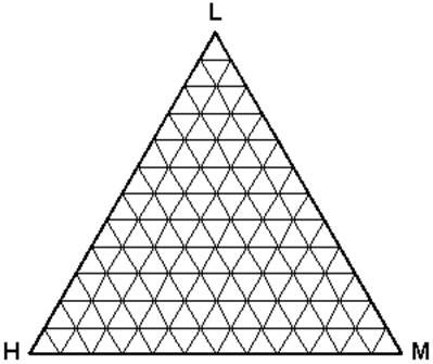
Intuitively, having more than two components poses a problem when a pictorial representation is desired. A rectangular coordinate plot, having only two axes, will no longer suffice. Gibbs first proposed the use of a triangular coordinate system. In modern times, we use an equilateral triangle for such a representation. Figure 5.6 shows an example of a ternary phase diagram. Note that the relationship among the concentrations of the components is more complex than that of binary systems.
Features:
- Any point within this triangle represents the overall composition of a ternary system at a fixed temperature and pressure.
- By convention, the lightest component (L) is located at the apex or top of the triangle. The heavy (H) and medium (M) components are placed at the left hand corner and right hand corner, respectively.
- Every corner represents a pure condition. Hence, at the top we have 100 % L, and at each side, 100 % H and 100 % M, respectively.
- Each side of the triangle represents all possible binary combinations of the three components.
- On any of those sides, the fraction of the third component is zero (0%).
- As you move from one side (0 %) to the 100 % or pure condition, the composition of the given component is increasing gradually and proportionally. At the very center of the triangle, we find 33.33 % of each of the component.
To differentiate within the two-phase region and single-phase region in the ternary diagram, pressure and temperature must be fixed. There will be different envelopes (binodal curves) at different pressures and temperatures. The binodal curve is the boundary between the 2-phase condition and the single-phase condition. Inside the binodal curve or phase envelope, the two-phase condition prevails. If we follow the convention given above (lights at the top, heavies and mediums at the sides), the two-phase region will be found at the top. This can be seen more clearly in Figure 5.7.
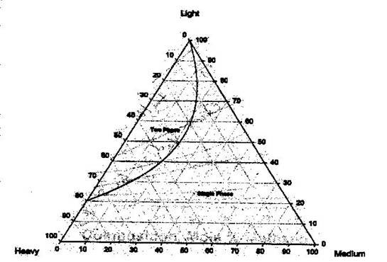
The binodal curve is formed of the bubble point curve and the dew point curve, both of which meet at the plait point. This is the point at which the liquid and vapor composition are identical (resembles the critical point that we studied before). Within the two-phase region, the tie lines are straight lines that connect the compositions of the vapor and liquid phase in equilibrium (bubble point to the dew point). These tie lines angle towards the medium-component corner. It can also be recognized that any mixture on a tie line has the same liquid and vapor compositions.
Finally, to find the proportion of liquid and vapor at any point on the tie line, we apply the lever rule.
Multicomponent Mixtures
For systems containing more than three components, pictorial representation becomes difficult, if not impossible. Simple diagrams can be obtained if the mole fractions of all but two or three components remain constant, and the variation of the two or three varying components with temperature and pressure are shown.
In practical applications, the mole fractions of all components can be expected to vary. For such systems, direct calculations based on physical models are the only way to obtain reliable information about the system phase behavior. This is the ultimate goal of this series of modules, and these calculations will be studied in detail as the course progresses.
Action Item
Answer the following problems, and submit your answers to the drop box in Canvas that has been created for this module.
Please note:
- Your answers must be submitted in the form of a Microsoft Word document.
- Include your Penn State Access Account user ID in the name of your file (for example, "module2_abc123.doc").
- The due date for this assignment will be sent to the class by e-mail in Canvas.
- Your grade for the assignment will appear in the drop box approximately one week after the due date.
- You can access the drop box for this module in Canvas by clicking on the Lessons tab, and then locating the drop box on the list that appears.
Problem Set
-
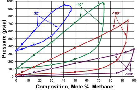
Figure 5.2 shows the P-T phase envelopes for eight binary mixtures of Methane and Ethane at eight different compositions. The data was experimentally generated at IGT (Institute of Gas Technology) and presented in the Research Bulletin No. 22. The vapor pressure curves of Methane and Ethane bound the phase envelopes of the eight binary mixtures of Methane and Ethane at different proportions. From left to right, these proportions (molar compositions) are:
P-T phase envelopes for eight binary mixtures of Methane and Ethane at eight different compositions Mixture Composition Mixture 1 97.50% CH4 and 2.50% C2H6 (closest to 100% pure Methane vapor pressure curve) Mixture 2 92.50% CH4 and 7.50% C2H6 Mixture 3 85.16% CH4 and 14.84% C2H6 Mixture 4 70.00% CH4 and 30.00% C2H6 Mixture 5 50.02% CH4 and 49.98% C2H6 Mixture 6 30.02% CH4 and 69.98% C2H6 Mixture 7 14.98% CH4 and 85.02% C2H6 Mixture 8 5.00% CH4 and 95.00% C2H6 (closest to 100% pure Ethane vapor pressure curve) Using this phase behavior data, generate the P-x and T-x diagram for Methane/Ethane mixtures at T = – 40 F and P = 500 psia respectively.
- If a certain amount of the mixture 40% C1 – 60% C2 is kept in a vessel at 500 psia, determine the temperature at which the vessel has to be subjected if at least 50% of the substance is required to be in the liquid state. How would your answer change if we were now required to have 10% of liquid in the vessel? How would it change if the overall composition is now considered to be 60% C1 and 40% C2 ?
- 10 lbmol of an equimolar C1/C2 mixture is confined inside a vessel at conditions of – 60oF and 500 psia. What is the percentage of liquid inside the vessel? What is the composition of the liquid and vapor at such condition?
- What would be the composition of the first bubble that appears in a isothermal expansion of a liquid at – 40oF? At which pressure would this bubble appear? What would be the pressure at which the first droplet appears in a isothermal compression of a vapor at – 40oF? What is the composition of such a droplet?
- Can you apply the lever rule to in a ternary diagram? If not, why not? What about a multicomponent system?