PT Behavior and Equations of State (EOS), Part I
Module Goals
Module Goal: To introduce you to quantification in fluid phase behavior.
Module Objective: To quantitatively and qualitatively compare ideal and real gas behavior.
Introduction
The ultimate purpose of this course is to build a firm knowledge of the phase behavior of fluids. With this understanding, we will be able to establish the basis and rationale upon which phase behavior applications in production systems are grounded. We are using the word production in a generic sense, that is, where it pertains to reservoir, pipeline, and the surface production (of any produced fluid).
So far, we have seen that much of the importance that we place on understanding phase behavior comes from the ability that it gives us to predict how a given system will behave at different conditions. We need phase diagrams to look at what the state of the system that we are dealing with is; that is, what is its original state. As a matter of fact, if we look at petroleum production, we often talk about a thermodynamic process that is taking place, involving a process path similar to one that we have seen in any basic thermodynamics course.
Just to give an illustration, consider Figure 6.1.

Production, as defined above, involves taking the reservoir from an initial condition (PA , Tf) to final state of depletion (PB , Tf), (PD , Tf), (PE , Tf) or even (PF , Tf). Once the end points of our thermodynamic path are fixed, the single most important question is determining the path that leads to such an end point. This path dictates whether or not you have the maximum recovery possible from the system.
When we talk about gas cycling, we are generally referring to the practice of injecting gas back into the reservoir. This is done in order to optimize the thermodynamic path we have chosen to take. In a typical condensate system, you generally produce a wet gas from the system with a high liquid yield at the surface. At the surface, you pass this gas through a series of separators; during this process liquid is going to drop out. The liquid that drops out will be rich in the heavier components. Hence, the gas that comes out of the separator will be dry (i.e., very light). If you inject this lean gas back into the reservoir, there will be a leaching process. All you are trying to do from the point of view of the phase diagram is to move the phase boundary and dew point towards the left (lower temperatures zones). Let me explain this in more detail.
Let us say that we have the phase envelope for the reservoir fluid shown in Figure 6.1, with the given path of production. If we were to follow the path from (A , Tf) to (E , Tf), we would enter the two-phase region and end up having liquid in the reservoir. However, you do not want liquid in the reservoir because its low mobility dictates that it would not be recovered! Next, you want to move that phase diagram to the left by injecting a lighter gas. When you inject a lighter gas, the phase envelope shifts to the left; your production path will be free of liquid dropout at reservoir conditions. By injecting the gas, we are making the overall composition of the reservoir fluid lighter. The effect of composition on phase behavior was discussed in the previous module (see Figure 5.2 in Module 5). This example demonstrates the importance of phase diagrams as tools that help us produce a reservoir in an optimal way.
So, we recognize that we needed phase behavior data for this particular system. The question now is how do we get the data? We can collect data in at least two ways: from laboratory measurements and from field measurements. Lab experiments are expensive, and we cannot hope to generate data for every foreseeable condition we may encounter. Just to give you an idea, generating a single phase envelope may cost at least $120,000. This is not something you want to be doing all the time. On the other hand, if you went to the field, you would lose valuable resources or have to stop operations to make your observations. On a routine basis, you don’t want to use the field or a lab as your main sources of phase behavior data. These options mean a lot of lost revenue and a great deal of expense. Is there a third option? Yes, indeed. We can rely on prediction, by which we produce a model that can do this work for us. In fact, we will be dealing with, and developing, this option in this course.
The basis for such a model is what is called an Equation of State (EOS). Hence, the central part of this course is EOS, since they are the basis of what we do in phase behavior.
There are several other examples that illustrate very vividly why we need to study equations of state. For instance, let us think about the concept of equilibrium.
In petroleum production, we generally make the assumption that, at every stage, the system is in equilibrium. When you think about equilibrium, you generally think about a system that is static, that is, not moving. When a system is moving, it cannot, in actuality, be in equilibrium. Nevertheless, the best approach we have so far is to describe it using equilibrium thermodynamics. While we usually assume equilibrium, we recognize that it is not a perfect assumption, but that it is a reasonable one.
This means that in the course of producing the reservoir, a process which always involves movement, I am assuming that everywhere the gas and the liquid are in equilibrium. With this assumption, we are free to use equilibrium thermodynamics, so we are able to employ EOS in describing the state of the system.
Consider the reservoir in Figure 6.1, in an entirely gaseous condition at (A, Tf), and having a known fluid composition zri (i=1,…n). As we produce this reservoir through a pipeline, we take the fluid from reservoir conditions through a battery of separators. Generally speaking, we deal with a series of separators, but for the sake of this discussion we will assume that we have just a single separator.
This separator does not care about the pressure and temperature of the reservoir. It only cares about its own pressure and temperature condition: Ps, Ts. The composition of the fluid at the separator inlet is assumed to be the same as that of the reservoir fluid, although this is strictly true only for single phase conditions.
The fluid exits the separator in two streams: a vapor stream and a liquid stream. As a petroleum engineer, we want to know how much gas, how much liquid, and the quality (compositions) of both streams. That is, we need quantitative and qualitative information. As we shall study in Module 12, we can perform a material balance around each separator to calculate the amount of vapor and liquid that is to be recovered. We will need the properties of both streams (such as density and molecular weight) in order to express flow rates in suitable field units.
How do we generate all this? We need a tool; that tool is an Equation of State! Why do we need an Equation of State? We need EOS to define the state of the system and to determine the properties of the system at that state. That is why it is called an equation of state. As you may have noticed, something critical in this series of lectures is the ability to establish links within all the material we are studying. We will not look at each topic simply as an isolated compartment, but instead, we must think in terms of how each piece of information fits into the overall picture that we are developing.
P-V-T Behavior
We embark now on a rather ambitious journey. Given a fluid, we would like to develop mathematical relationships for predicting its behavior under any imaginable condition of pressure, temperature and volume (P-V-T). In other words, we want to describe the P-V-T behavior of fluids in general.
As we stated earlier, this is a very challenging problem. The way science approaches these sorts of problems is to introduce simplifications of the physical reality. In other words, we formulate a set of assumptions and come up with a base model that we might call ideal. From that point on, once the base model has been established, we look at a real case by estimating how close (or far) it performs, with respect to the base (ideal) case, and introducing the corresponding corrections. Such corrections will take into account all the considerations that our original assumptions left out.
Let us discuss our base case for fluids (the simplest fluid we may deal with): the ideal or perfect gas.
Ideal Behavior
An ideal gas is an imaginary gas that satisfies the following conditions:
- Negligible interactions between the molecules,
- Its molecules occupy no volume (negligible molecular volume),
- Collisions between molecules are perfectly elastic — this is, no energy is lost after colliding.
We recognize that this fluid is imaginary because — strictly speaking — there are no ideal gases. In any fluid, all molecules are attracted to one another to some extent. However, the ideal approximation works best at some limiting conditions, where attraction forces can be considered to be weak. In fact, ideal behavior may be approached by real gases at low pressures (close to atmospheric) and high temperatures. Note that at low pressures and high temperatures, the distance between any pair of gas molecules is great. Since attraction forces weaken with distance, we have chosen a condition where attraction forces may be neglected. In conclusion, we consider a gas ideal when each molecule behaves as if it were alone — molecules are so far apart from each other that they are not affected by the existence of other molecules.
The behavior of ideal gases has been studied exhaustively and can been extensively described by mathematical relationships.
For a given mass of an ideal gas, volume is inversely proportional to pressure at constant temperature, i.e.,
(6.1)
This relationship is known as Boyle’s Law. Additionally, volume is directly proportional to temperature if pressure is kept constant, i.e.,
(6.2)
This relationship is known as Charles’ Law. By combining both laws and recognizing “R” (the universal gas constant) as the constant of proportionality, we end up with the very familiar equation:
< (6.3)
This represents the equation of state (EOS) of an ideal gas. Numerical values of “R” depend on the system of units that is used:
If we construct the P-v diagram for an ideal gas at a given temperature, we end up with the isotherm shown in Figure 6.2.
The ideal gas model predicts two limiting fluid behaviors: first, that the volume of the gas becomes very large at very low pressures as , a concept that agrees with what we know from our experience in the physical world). And second, as (the volume of matter just “vanishes” if the pressure is high enough: this concept we would not be as willing to accept). These two behaviors are a consequence of the assumptions made in the ideal gas model.
Real Gases
In reality, no gas behaves ideally. Therefore, the ideal EOS is not useful for practical applications, although it is important as the basis of our understanding of gas behavior. Even though the ideal model is not reliable for real engineering applications, we have to keep in mind that the ideal gas EOS is the starting point of all modern approaches.
If we look back at Figure 6.2 and recall our discussions about P-v behavior of pure substances, something should catch your attention. Figure 6.3 shows us the typical P-v behavior of a pure substance to facilitate our discussion.
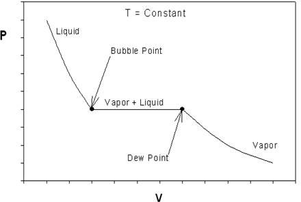
What can we conclude about the ideal EOS while contrasting Figure 6.2 to 6.3? The curve in Figure 6.2 is continuous; Figure 6.3 has an obvious discontinuity (at the vapor+liquid transition). Hence, one thing we can already say is that the ideal EOS is at least qualitatively wrong. For a real substance, as pressure increases, there must be a point of discontinuity that represents the phase change. Ideal gas will not condense, no matter what pressure it is subjected to, regardless of the temperature of the system. In other words, we cannot hope to reproduce the P-v behavior of Figure 6.3 using the ideal equation (6.3) since no discontinuity is to be found. However, the real P-v isotherm can be approximated by ideal behavior at low pressures, as we can see from the plots.
We can also establish some quantitative differences between ideal and real PVT behavior. For example, for most conditions of interest at a given volume and temperature, the ideal gas model over-predicts the pressure of the system:
(6.4)
We can explain this difference by recalling that a real gas does have interaction forces between molecules. Secondly, we recall that the concept of “pressure” of a gas is a consequence of the number of molecular collisions per unit area against the wall of the container. Such number of collisions is, in turn, a measure of the freedom of the molecules to travel within the gas. The ideal gas is a state of complete molecular freedom where molecules do not even know the existence of the others. Hence, a hypothetical ideal gas will exert a higher pressure than a real gas at any given volume and temperature. When molecules come together (real gas), it reduces the available free space for the molecules and pressure is reduced.
Additionally, the ideal model assumes that the physical space that the molecules themselves occupy is negligible. In reality molecules are physical particles and they do occupy space. Once we find a way of accounting for the space that the molecules themselves occupy, we would be able to compute a “real” free volume available for the molecules to travel through the gas. In the ideal case, this free volume is equal to the volume of the container itself since molecular volume is not accounted for. In the real case, this free volume must be less than the volume of the container itself after we account for the physical space that molecules occupy. Therefore:
(6.5a)
(6.5b)
Summary
The ideal gas EOS is inaccurate both quantitatively and qualitatively. Quantitatively, ideal gas will not condense no matter what pressure and temperature the system is subjected to. Quantitatively, pressures and volumes used by the ideal gas model are higher than the values that a real gas would have. These are the primary reasons that scientists have made an effort to go beyond the ideal gas EOS, simply because it does not apply for all the cases of interest.
Action Item
Answer the following problems, and submit your answers to the drop box in Canvas that has been created for this module.
Please note:
- Your answers must be submitted in the form of a Microsoft Word document.
- Include your Penn State Access Account user ID in the name of your file (for example, "module2_abc123.doc").
- The due date for this assignment will be sent to the class by e-mail in Canvas.
- Your grade for the assignment will appear in the drop box approximately one week after the due date.
- You can access the drop box for this module in Canvas by clicking on the Lessons tab, and then locating the drop box on the list that appears.
Problem Set
-
Under what conditions should a real gas behave as an ideal gas?
-
Can we manufacture an ideal gas?
- Write a paragraph on what you think we should do with the ideal gas equation to make it applicable to real gases. Describe all the considerations that you feel must be accounted for.