To model the mineral dissolution/precipitation, we need to inform the code both reaction thermodynamics and kinetics. Here we introduce how to set up simulations for mineral dissolution/precipitation in a well-mixed batch reactor, where the concentrations of all species and temperature are assumed to be spatially uniform. That is, the rate of mixing is faster than the rate of dissolution or precipitation, which is in general true for most minerals except carbonates under very low pH conditions. No transport processes and boundary conditions need to be defined because of the assumption of uniform concentration. The example 6 included in the CrunchFlow package is also a good reference for kinetic reaction setup.
Example 2.1: Calcite Dissolution
Calcite dissolution proceeds through three parallel pathways as shown in reactions (1)-(3). In addition, a series of fast aqueous complextion / speciation reactions occur simultaneously. These fast reactions are similar to those in the examples in the lesson on Aqueous Complexation.
In a batch reactor of 200 ml, the initial solution is at a pH of 5.0 with close to zero salinity. The initial total carbonate concentration is . The kinetic rate constant for three parallel reactions are , and respectively. The volume fraction of the calcite grains in the batch reactor is 0.5%, with a specific surface area (SSA) of 0.24 m2/g. Please set up the simulation and plot the following quantities as a function of time:
- Total Ca(II) and total inorganic carbon;
- Individual Ca-containing species and carbonate species;
- pH and the saturation index
Here is a light board video (12:44) of what equations the code solves for this system.
Mineral Dissolution & Precipitation
PRESENTER: So in this video we're going to talk about mineral dissolution and precipitation, the equation involved and interaction involved. This is different from the previous lesson, aqueous [INAUDIBLE], because the previous reaction only involved reaction [INAUDIBLE] dynamics. Meaning we care about the end point of the reaction.
When we have mineral dissolution precipitation, because reaction usually occur at the interface of solid phase and water, reaction occur much slower. So we often need to consider the kinetics of the reaction. Meaning we care about how long it takes for the reaction to occur to reach the end point.
So what I'm going to do today here is using the carbonate dissolution system in a battery reactor. So battery reactor, meaning it's closed while mixed, so that it does not have constitution gradient in different parts of reactor. So essentially you're solving for one constitution for each species for the whole reactor. So that's our systems.
If you think about if you want to draw something relevant to what you do in the lab, but you think about these water, and then you have these calcite grains, and you have these mixers that will keep the system well-mixed. And again, the reaction involving this system is similar to what we talked about last time for the aqueous speciation. The carbon and water-- for example, all these three reactions are the same as what I wrote before. Invest in one. But the key thing is we are adding this calcite dissolution, which is calcite dissolving out to become calcium and carbonate.
Calcite or carbonate in general is a very common type of rock or mineral fissure or surface. So it's a reaction. Compared to the aqueous speciation or [INAUDIBLE], it's much slower. But compared to other type of mineral dissolution, it's actually reactive fast.
So we have these four reactions here. You can think about the calcite dissolution essentially kind of releasing out the elements from the solid phase the water phase. So it dissolve as an add to the water with calcium species and carbonate species. But then once carbonate is released into water, it quickly goes through the speciation reaction to become either bicarbonate or carbonic acid, depending on the pH a system, as we talked about last time.
So if you think about the species in this system, now that the species we have, in addition to the five species, carbonic acid, bicarbonate, carbonate-- this is wrong. So it should be carbonate. And this should be two.
So you have these three carbonate species. You have hydrogen ion, which minus acid five, as before. But on top of that, you are adding calcium.
So essentially, now you have six species. You would have Ca2 plus carbonic acid carbonate, bicarbonate carbonate. And then you also have H plus or H minus. So that's six species.
So what does that mean, is that we essentially have six unknowns to solve for. And we will need six equations to solve for this, to solve for the species. But notice that one things that we need to pay attention to is that we have these three reactions that occur fast.
So you have these three equations already there. We can think about as one, two, three. That is as a three relationship. But we cannot use this one, because this is not a faster reaction. These are fast reaction.
This is a slow reaction, which means we need to care about its kinetics. Like how far it release as these chemical species over time. So when we solve these equations, we actually need to consider these time component.
In this case, we will need to think about the mass balance of system. So these calcite dissolving out and release out. For example, Ca2 plus, and releasing out CO3 bicarbonate. And then this will be exchanged into bicarbonate and exchange into carbonic acid. So these three specie are exchangeable.
So when we think about mass balance of system, you would think about the constitution of a single body calcium first. Volume-- this is a volume of the water in the system. And you have the constitution of calcium.
Ultimately, we are solving for contrition, not activity. So this will give you the mass. So contrition of the unit and mass per volume. And then we will need to solve for order and differential equation now because just time component here. So in this kind of system we don't really have fro transport so the only source of zinc of this calcium specie is through these reactions.
So let's say we have a rate constant of this reaction is Ksp. So that's the rate constant. And we talk about the tst rate, which is transition state rate theory in the online material. So you can go look this up.
So this Ksp and this is rate constant times a surface area of the mineral. And then times for example, how far away the reaction is from equilibrium, which will depends on the activity of Ca2 plus activity of carbonate, and then divided by Ksp, which is how far away this is from equilibrium. So this is Iap.
Now when we have dilute system-- if we have dilute system, then this activity would be equal to c. So you can replace every a is c for simplicity. So essentially, is this equation saying mass of calcium is added to system, to the water, by having this rate lower for calcium. But we also will have adding total carbon to the system. So similarly, you will have V, d, and then we call it total carbon cT, dt.
It will have the same expression here as Ksp A or minus activity ca. Because, essentially, it's through the same reaction. So this rack essentially adding calcium total carbonate-- this CT will be equals to again, constitution of carbonic acid plus concentration of bicarbonate and concentration of carbonate.
But then we need one more equation. One, two, three. And then this is four, this is five. We need a six equation, which would it be-- if you think about it, when this mineral dissolving out to form calcium and carbonate, it's actually changing the pH of the system. So the hydrogen ion-- or somehow we also call it's a measure of acidity of system will also change.
I'm not going through the detailed derivation of the whole process how we come up with. But let's call this dC, which is-- so this a constitutional cT-- concentration of hydrogen ion total dt. And by dissolving out calcite, actually decrease acidity of system. So it will actually have minus Ksp. And then activity one minus a Ca2 plus.
So again, it's the same rate law, but it do actually have the minus signs. That meaning it's decreasing the total acidity of a system. So the expression for the total acidity will be different if we define different to comnination primer specie.
But in general, if we define this carbonate as a primary species, we should have HT equal to hydrogen, concentration hydrogen ion. This should be CHt. Hydrogen ion plus concentration of H2CO3 minus concentration of bicarbonate and minus concentration of OH minus. You can actually derive this equation from the [INAUDIBLE] method. And these expressions is actually-- you can look at [INAUDIBLE] And by combining different terms, you come up with this. So essentially, we have six unknowns, and you have six equation to solve with that. But on top of that, one thing we need to pay attention is that these are OD equations.
So we call it ordinary differential equation. Differential equation, meaning we have one independent variable, which is time in this equation. So typically, the code will be solving these equation first using time stepping.
And then once we get the concentration calcium, concentration of CT, concentration of CHt, you have three kind of variable in particular time step. And then we solve for the algebraic and relationship with these numbers together with these three relationship. And by doing that, we essentially get the concentration of all the six species as a function time in these aqueous species. And what do you see? For example, your homework is essentially generated by solving these equations.
Here is a video demo in CrunchFlow on how to set up the simulation in CunchFlow (43:51 minutes).
Li Li: OK, so let's start. This is lesson 2 on mineral dissolution and precipitation. Now, with example 1, it's to set up as if you are doing a batch reactor experiment with some calcite grains in the solution. And you essentially will be running numerical experiments, imagining that your calcite dissolution rates are in these given numbers-- you have how much calcite grain in the system, et cetera.
So here-- let's see. For this lesson, the difference between this one and previous one in lesson 1 is, lesson 1 only have aqueous complexation. So it doesn't have any kinetics, it only has thermodynamics. The other one is zero-space dimensioning, and also, no-time dimensioning.
Now here, by introducing the reaction kinetics, we are essentially now looking at it as a time dimension. We'll still have a well-mixed system, which is a zero-dimensional system. We're not looking at things change in the functional space, so you have uniform contusion in the batch reactor.
So that's a major difference. Let's read the example question, and then I would explain a little bit, and we can try to set it up in CrunchFlow. OK, so example 1 is about a calcite dissolution. Calcite dissolution proceeds through parallel pathways, as shown in reaction 1 to 3. That's what we have-- we're seeing lesson 2.
In addition to these kinetic reactions, there are also a series of instantaneous aqueous complexation reactions, that occur at the same time. The three fast reactions should be the same as the ones in the example 2 of lesson 1. Also, that's for these fast reactions on the aqueous speciation reaction. So this essentially specify what aqueous speciation reaction you should include in this example.
Now, in a batch reactor, the initial solution is at a pH 5.0, with close to 0 salinity, meaning it is not a constituted solution. The initial total carbon concentration is 3.15 times 10 to the minus 4 mole per kilogram water. Kinetic rate constant for three parallel reactions are 1.00 times to 10 to the minus 2, 5.62 times 10 to the minus 6. And then the other number-- this is for the corresponding three reactions in 1, 2, 3.
And then the volume fraction of the calcite grains in the batch reactor is 0.5%. So if you have 100 milliliter, then you have 0.5 milliliter of calcite. You can convert that to how much mass is this with a specific surface area of 0.25 meters squared per gram. Please set up the simulation and plot the following quantities as a function of time.
So now we're looking at the time dimension, right? We're starting from the initial condition. So initially, you have some total carbon concentration there-- 3.15 times 10 to the minus 4 mole per kilogram. But essentially there, you don't have other species.
Now, the question it's asking you, first of all-- so total calcium concentration and total inorganic carbon. So you need to plot that as a function of time. Second was the individual calcium-containing species. And carbon is species. And so here, you want to see, essentially asking, which one the dominant species and everything. And then also, the pH and IAP over Keq, which is a saturation index. Maybe that-- make it more explicit.
OK, so let's do this. Let's go to that folder again. OK, again-- so I have four files here waiting for you. Let's open the input file. Oh, I hate it when-- let's do it in Notepad. I don't like all these red line and everything-- underlining all my words. Let's open it with Notepad. OK. Much better.
All right, so this is a template, essentially. And we need to fill in, OK? So this did not say TITLE will be "lesson 2-- calcite dissolution in a batch reactor." These runtime specifications are still there. Database-- make sure it's datacom.dbs and everything. OK.
So here, make sure you don't do speciate only, because when you do speciate only, the time is not going to be stamped, and you cannot do this calculation. Because this is for kinetic, and you want your time stamping Output file-- the output procure block. We need to specify what we want the system to output.
So first of all, we need to specify, what units are we using? Let's do seconds. We know calcite dissolution very fast-- or maybe minutes. Let's do minutes. And let's call it time. We need to specify time series. And let's call that calcite dissolution .out.
And for batch reactor, we should only have one group block. So let's just specify this as a group block 1. Time series print. So what time series print do is, you specify what species you want to print. So you can put a specific freedom-- calcium.
And this need to be the-- I'm just going to make it explain. Needs to be primary species. It cannot output times there for secondary species. So we can specify it's the calcium pH or bicarbonate. But it's very important that maybe we'll do all-- "all" meaning all primary species would be printed out.
Discretization-- we should only have one species, right? So first, we need to specify the units' distance-- units. Let's say it's meters. And then, when you need to specify kind of zones-- x-zones, y-zones. So you have x-zones should be 1.1. So you only have one group block.
Now, for the other dimensions-- if you only specify 1, so that essentially you have 1 meter, 1 meter, 1 meter. If you don't specify other, it will assume it's meter-- the same units-- and it's 1. Quantity is 1. So essentially, you have 1 meter cubed. Maybe we'll make it centimeters, just to be more realistic.
And you have 10.0. It shouldn't matter, because we are specifying volume fractioning, not a specific number. And so if I'm specifying-- maybe I will do 100. Because a typical batch or a flux or something, that you would do batch reacting as hundreds of milliliters. So I'm specifying here-- this is 200 centimeter cubed, essentially. The other two dimension-- y-direction and z-direction into it-- by default, it will be 1 centimeter, 1 centimeter. So it should be 200 centimeter cubed-- essentially 200 milliliter. That's the discretization.
Now, we actually also need-- in output, we need to specify how long we want this to run-- spatial profile. So maybe we'll do, let's say, 1 minute. And then, maybe 20 minutes? 10 minutes. OK. Maybe 10 minutes. It is out pretty fast. Let's see. It's 5.0, 10.0, 50.0. All right. So we run it for 100 minutes. So it's the end point time. So this submission would be run until 100 minutes.
Now, we don't have spatial discretization. We don't have. We only have one group block. It's a well-mixed system, so we don't need to specify-- we don't have something coming from the boundary. We should be fine. So let's specify-- initial conditions should be whatever condition we specified it. So let's do it later.
We don't have transport. We can safely delete that. We also don't have flow, we don't have porosity. We can now delete all of that. So the primary species you want to put in, we talked about before. You should have calcium. First of all, all we need-- H plus, actually. What else you need? I'm going to look at the question again.
Let's put a bit of sodium chloride there, just in case we need-- to make charge balanced, we can use sodium chloride. So usually, you use species that are not reactive to do charge balance. Otherwise, you would be changing the condition we put in the species.
What else? And we need bicarbonate speciates-- still use bicarbonate. That should be it for primary species. Second species-- again, OH minus would be the top one. Or the other carbonate species-- A, Q-- 0 3. Potentially with these, we could form COH plus-- that's another aqueous species.
You can check by doing speciation only-- by data sweeping or something-- to see which species will be dominating, if you would like. But that's your calcium. Carbon we also form-- aqueous calcium carbonate. And if you would have carbide, possibly you would also have that. OK, I think that's good for our second speciate, I believe.
OK. So for this one, we need initial condition. Because the system started with-- this is where t equal to 0. So let's call that condition initial. And you will need all the prime-- you need to specify all the primary species, so copy the list of primary species here.
So question says, initial pH is 5.0. So let's specify pH would be 5.0 first, instead of saying H plus. Let's do 5.0. So initial calcium concentration should be almost 0. Now usually, I try not to put directly zeroes there, because sometimes computers have problem with 0. And I always put a very small number there, just in case. So for the very small-- essentially none-- I'm putting very-- these 10 to minus 10 concentrations. All right.
Bicarbonate is a good-- the question said, initially, it's 3.15 times 10 to minus 4. OK, they say what you put in there. That's the total concentration saturate, not specific. And question says, total carbonate concentration. That's consistent.
Now here, we also have either-- in solution, we should also have calcite, because calcite need to dissolve out. So we need to have the calcite mineral. This is very important, because otherwise, there would be no representation calcite going in there. So let's put calcite. And it says, volume fraction is 0.05%.
So the first number should be the volume fractioning. And then, it also says, specific surface-- the key word is specific-- surface area is 0.25. So let me just comment on that. The first number, volume fractioning, is 0.05. This SSA is 0.24 meter squared per gram. So that's the unit.
You can also specify total surface area, I believe. Let me just search the manual. I believe you can do-- this should be similar. Oh, you can specify BICG surface area or specific surface area. If it's BICG surface, you'll be putting the absolute value. If it's specific surface area, it should be in the units meter squared per gram.
So it's the typical-- the way you're putting is, name of solid face, volume fractioning, surface area option, and value. BICG surface area. So you can look through these if you would like to have more details. Go into page 68, 69 in the manual. All right.
Now, we cannot put in the grain size. But the specific surface is more or less refracting the grain size you have. When you have small grains, you tend to have larger specific surface area. And when you have larger grain, you have small specific surface area. But also, of course, for different mineral, they're also different. OK. So the initial condition.
But one thing we're keeping-- we need to keep in mind is that the solid face need to be recognized by the mineral-- key word, block. This is where you're putting the kinetic information. Without that, you will either use the kinetic information grid block, or in the database-- which I usually prefer to putting input file, because then you have everything in the same place.
So here, you will need to put in the rate constants in the log 10 units. These rates should be in log 10 rates in units of mole per meter squared per second. All right? So the way you're putting is calcite, and then you have the label, if it splits it using default.
Then your rate is-- OK. Let me just check the three reaction pathways. We are saying, for calcite, you have these three reactions. So you have k1, k2, and k3. They all have the same-- so one is, k1 depends on each process. k2 depends on H2O CO3. k3-- there's no dependence. So let's just also check the database.
Let's save it, and let's look at database. Make sure it's a default in everything. Make sure we know what are the format for each label. Search for calcite. OK. So this said, T-S-T rates are-- default is-- OK. H plus 1 is one that depends on each process. That's the k1, right? So let's see, label. So you need to look back and forth a bit. So let's do H plus first.
And I said, the rate constant is what? 1 times 10 to minus 2, for the 3 or 4 k one. OK, for the H plus dependence once. So this one is-- in units of mole per meter squared per second. So this one should be minus 2. And then, you have the-- so second one is-- let's call it a CO2, so it's less confusing. Let's call it a CO2 dependence. And it's dependent on this with 1.0.
So this dependence need to specified in the database, but not the one-- so I probably should say H2O3. And then, the default is 1 without any dependence. OK, so if we specify the number here-- OK, so that will be CO2. And then rate.
So the second rate constant is 5.62 times 10 to the minus 6 in log unit. Let me just-- 5.62. OK, 10 to the minus 6-- minus 6. So it's 5.25. All right. And then, the default ones without dependence is 7.24 times 10 to the minus-- so 7 point. Minus 9-- minus 8.14. For the three parallel reactions-- 1, 2, and 3. OK.
So now, what-- so these rate constants should be override to whatever that is in the database. OK, you have condition-- let's just check it. You have a condition-- you have mineral specified with kinetics. You have primary and second species. OK, you need to specify what are the initial condition.
So you should have say, initial condition-- initial, we call it-- yeah. We called that initial. So this condition will be in the first code block. We only have one group block. This is specify the location and-- you can dig into manual for them-- search for this key word block, and the manual explain in detail what you can put in.
So here-- this initial condition is interesting. OK, I'm using this initial condition for this group block 1. Let's see if they run. I think you should. And so I made a mistake somewhere. So that's 2 lesson, example 1. Oh-- rate label. Cannot have enough on-- in database. Looking for calcite rate label CO2. Let's see. Hm. Interesting. Maybe I didn't save it.
OK, let's do it again and just save it 2 lesson example. Now it runs. There's something else coming up. So the other time I changed it, the to CO2, but I didn't save it. So the code doesn't recognize the CO2 label. So I save it to the database with the CO2. Then the code not recognize that label.
And then, now is speciation-- OK. So it-- speciation is finished. No aqueous kinetic block found. Retardation parameters not found. Both the number of cells and the grid block spacing should be-- oh, OK. Only one value provided. Yeah, I've seen the problem with discretization. So I need to provide-- let's go to-- just make sure we-- discretization key word block-- x-zone, y-zone, z-zone.
OK. At discretization, you can specify x-zone, z-zone, y-zone. So the syntax is-- it's supposed to say x-zone. And it's how many number of cells and spacing. OK, good. And number of cells should be integer, and spacing is a real number. So we are saying, we have one group block. And the spacing is-- it's 200 centimeter. I think that should make it work. Let's try it again. So I just look it up and do it again.
All right. So the runs is finished. That's good. OK. And suddenly, you discover there are a lot of output files. Each of these output file-- for each of these-- these are all out, right? So you have each of these every time. You have every 1, every 2, every 3, 4, 5. Each of these is corresponding to one of these times that you specified in the spatial profile. Remember, in spatial profile, I put 1 minute.
So it's spit out the output at 1 minutes, 5 minutes, 10 minutes, 50 minutes, and 100 minutes. So the 1 will be representing 1 minutes. 2 will be 5 in this. So each of these have 5. Right? I said 2, perhaps there is 5. Concentration have 5. Guess mineral percentage, because you have mineral. pH, porosity-- a lot of information.
OK, these are standard operations. Some of them are not useful for this example. But I want to-- let's go through. So you don't have to answer questions at these. You want to print-- plot everything in the function of time. All these other areas-- like, area 1 to 5-- because we only have one grid block. So the spatial profile is not really useful for us.
If we have 100 grid block, we want to see how this varies spatial rate. Now you only have one grid block. So it's not really interesting. It's more interesting to look at that as a function of time. And then we specified the breakthrough curve should be in-- OK. Calcite dissolution data out. So let's look at that file. This will be what you should look for for the breakthrough.
Calcite. This-- OK, this good. So as we said, essentially output everything, right? OK. So again, first it's time stepping varied with very tiny time steps. And then, later, it becomes more larger times then, because it's approaching to equilibrium.
Now look, and so you have pH, you have H plus, calcium, sodium chloride, always a function of time. We said "all," so it also spit out sodium chloride. But we actually don't really need that. But why-- OK, we also should have-- OK. Hm, interesting. Bicarbonate, H plus, CO2, AQ, 03, calcium. So it actually does spit out all the aqueous speciation, as well.
And these are inactive variables. These are in, actually, log units. For the primary species, it's an absolute value. It's not log. For the second species there, you log in log. So this, it would be 10 to the minus 8.99, 10 to the minus 3.52, 10 to minus 9.5, for example. So they should be increasing.
So you actually can directly read, if you want, to plotting. So you can either do Matlab, Excel, whichever ways are the easiest for you. Let me just show you how to open that in Excel, so if that's easiest for you. I'm opening up Excel. And I will say, Open. Hm. Why don't you-- oh. It's says no book. Sorry.
OK, let's do this one-- let's see how. OK. So you would say, so the code, I can actually fix the widths. It will space out for this. OK, it probably doesn't matter. OK, so you have all the different species-- pH, H plus, pH. So you can plot-- whichever that I asked for you can plot. Problem is species. Pay attention, there's this thing.
OK, so this also give the calcium in the log units. So these are individual species, and these are the total for the primary species. So if you want to plot a primary species, like the individual species, you do want to use these columns, starting from H plus here, when it has a log-- after it's already been log.
So this is how you can do, for example, getting all the time series and plot out the files. So that's an example. You can see all the change in the function of time, how the saturation changed the function of time. So here, I'm giving you the solution already, but you want to be able to generate that by yourself. I want to be able to see that.
And you shouldn't just-- before you do anything, you shouldn't look at this solution yet. But I'm still telling you, here-- these solutions, OK. For the individual concentrations, OK, these are total calcium, total bicarbonate. So it should be from the first several columns on primary species.
And you can see, the carbon is always higher than the calcium, because initially, there is some carbon in species there. So if you look carefully, the difference is actually exactly the initial concentration of carbonate. Because essentially, the calcium-- when the calcite dissolves, it should be dissolving calcium and total carbon in one-to-one stoichmetric coefficient.
When the calcite dissolves, pH increases over time, until it reach around 8, so it's concentration in which certain values stopped, because it reach equilibrium. IAP over Keq get to about 1, which is at equilibrium at about 120 or 130 minutes, which is similar to where concentration reached a plateau.
And looking at the individual concentrations-- so this is a bit hard to see. Total calcium should be the highest, and blue is-- so the free calcium is a dominant species. And then this light blue, you see it-- bicarbonate. So calcium bicarbonate is the second one. Red one is Ca CO3, and then you have COH plus, which is reasonable, because you have a lot of carbonate species in the system.
So that should give you a sense of how you would do with the mineral dissolution precipitation. And as an extension of the example 1, in the homework assignment, I asked you to do the carbon dissolution, changing several key parameters, essentially.
Example 1 did all this in one particular condition. But we all know, in the lessons, we discussed where the constant is important, surface area is important. Initial pH, salinity-- all these things are important. So how do they change the dissolution process, if we change these numbers? So in every question of these, it asks you to change your numbers, and compare three different cases, in term of how things are different with different sets of parameters.
And then, the question 1 is about feldspar dissolution. So in example 1, give you everything about calcite. In question 2, you are supposed to calculate to set a feldspar dissolution using the figure 7 in Blum and Stillings, with the rate dependence on H plus, OH minus, or the neutral one without any pH dependence. And you should be able to study that up to run these simulations.
All right, I think I'm going to stop here. And I hope you have fun playing with CrunchFlow in setting up mineral dissolution precipitation. Again, this is in batch reactor. So imagine that you are doing a numerical experiment of the batch reactor, and you're putting calcite grains-- different grain size.
So you have larger, smaller specific surface area, and all that. OK, I'm going to stop by, and hope you have fun here. And we can discuss later, if you have questions. OK.
Figure 4 below shows the evolution of aqueous chemistry during calcite dissolution. Total Ca(II) and carbonate increases over time and should follow the 1:1 stoichiometric ratio. However, total carbonate concentration is higher due to the initial presence of total carbonate at the concentration of . The individual speciation of Ca(II)-containing species are in D shows that Ca2+ is the dominant species. During the dissolution, pH and increase over time, until reaching close to 1 at about 100 minutes, after which the system stabilizes and no more dissolution occurred after that.
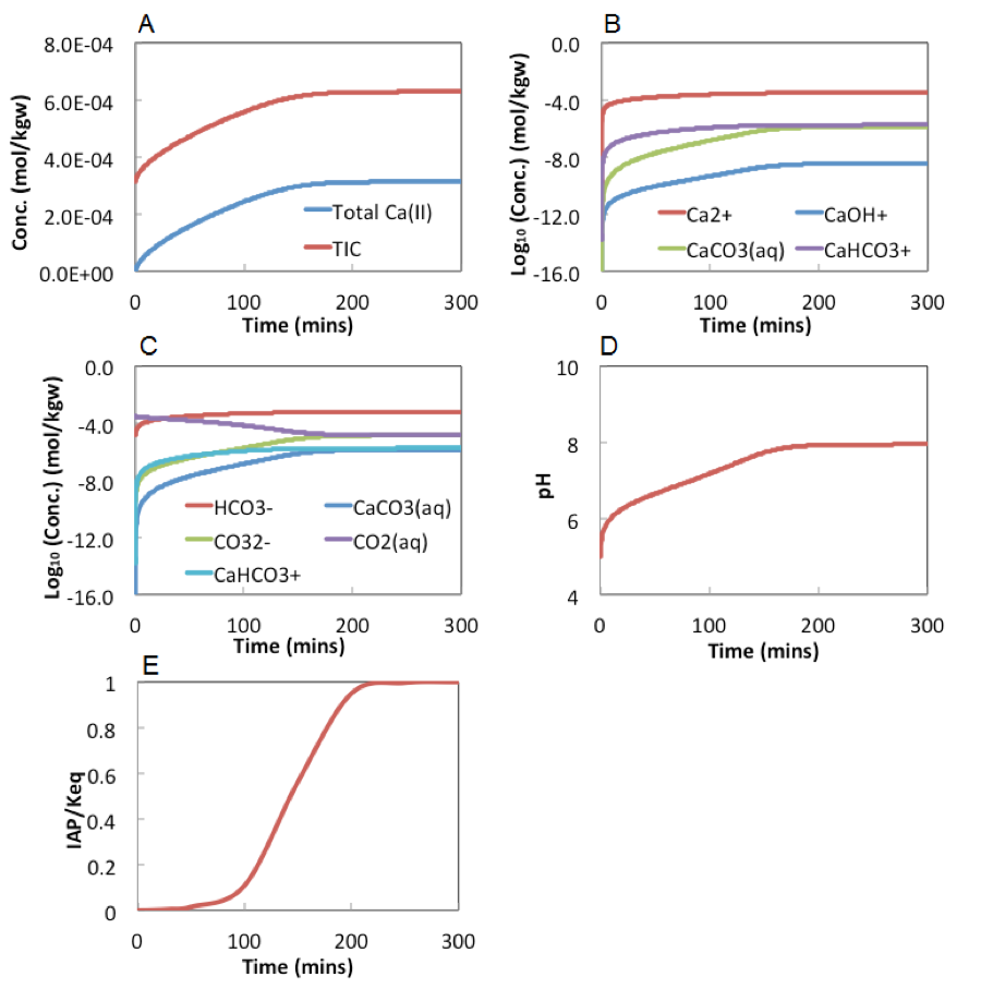
As can be seen from these figures, the dissolution reactions reach equilibrium at about 200 minutes, where pH increases to about 8. Total Ca(II) include Ca2+, CaOH+, CaCo3(aq), and CaHCO3+, with Ca2+ being the dominant species (shown in figure 4B). Total inorganic carbon includes CO2 (aq), HCO3-, CO3--, CaHCO3-, and CaCO3(aq). HCO3- is the dominant species at most of the time except very early time when pH is still at about 5, where CO2(aq) dominates.