Lesson 10: Mineral Dissolution in Two Dimensional Systems
Overview
In this lesson we will set up 2D reactive transport systems in both homogeneous and heterogeneous domains. You will learn 1) how physical and geochemical processes are coupled, and 2) how spatial heterogeneity controls reaction processes. In essence, this lesson combines 2D transport and mineral dissolution and precipitation lesson. Please review these two lessons if necessary.
Learning Outcomes
By the end of this lesson, you should be able to:
- Understand how mineral dissolution and transport are coupled;
- Set up simulations in Crunchflow with flow, solute transport, and mineral dissolution and precipitation reaction in 2D homogeneous and heterogeneous systems.
10.1. Introduction
In this lesson we are not going to introduce new concepts. The flow and transport processes in homogeneous and heterogeneous systems (1D and 2D) have been introduced before. Similarly, mineral dissolution has also been discussed in a previous lesson. These processes are typically coupled in heterogeneous porous media, meaning they can affect each other. That is, flow influences reactions, and reactions can also have impacts on flow.
In a system where both physical flow and transport and reactions coexist, a general governing equation for any dimension system is as follows:
where Φ is porosity, Ci is the concentration of a primary aqueous species i (mol/m3), D is the hydrodynamic dispersion tensor (m2/s), u is the flow velocity (m/s), ri,tot is the summation of rates of multiple reactions that the species i is involved (mol/ m3/s) , and Np is the total number of primary species. Solving Np equations simultaneously gives the concentrations of primary species at different time and locations, which can then be used to solve for the concentrations of secondary species through laws of mass action (equilibrium relationship of fast reactions).
The equation (1) is general for systems with different number of dimensions (one, two, or three dimensions). Note that this is similar to the governing equation that we discuss in the 1D chemical weathering lesson, except that here we do not specify the dimension. If we specify this for 1D system, it will then be the same from as the governing equation in the 1D chemical weathering lesson.
Also note that in this equation, the dispersion coefficient and the velocities are written as tensors or matrix (in bold symbols) and can have different values in different locations. In fact, all porous medium properties, including porosity, permeability, and surface area can have spatial variations, as we will see in the example.
10.2. Setting up magnesite dissolution in homogenous and heterogeneous columns
Here we will build upon example 8.1 in lesson 8 to illustrate a magnesite dissolution example in homogeneous and heterogeneous 2D systems based on the experiments in Li et al. (2014). I am reiterating the example 8.1 here.
Example 11.1
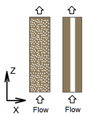
The following gives an example of setting up flow and transport calculations in 2D homogeneous and heterogeneous domains. Here we use the physical set up of 2D cross-sections of the Mixed and One-zone column in (Li, Salehikhoo et al. 2014). The authors packed 4 columns of 2.5 cm in diameter and 10.0 cm in length with relatively similar amount of magnesite and quartz distributed in different spatial patterns. Here we focus on two columns that represent two extreme cases: the Mixed column with uniform distributed magnesite and quartz, as well as the One-zone column with magnesite all clustered in one cylindrical zone of diameter of 1.0 centimeter. To keep it simple, here we will do the calculation for 2D cross-sections, instead of following the steps in section 3.2.4 in the paper to convert 2D to 3D. So our numbers might be different from the paper. We are also assuming that in the middle one zone magnesite is 100% of the solid phase and the Mixed column has the same total amount of magnesite as in the One-zone case. The 2D system has a size of 25 mm by 100 mm. A constant differential pressure is imposed at the boundaries in the z (vertical) direction, leading the primary water flow direction in the z direction from the bottom to the top. No flux boundaries are specified in the X direction (Li, Salehikhoo et al. 2014).
| Columns | Mg zone | Qtz zone | 2aL (cm) |
4aT (cm) |
ke (× 10-13m2) |
Φ avg |
|---|---|---|---|---|---|---|
| Mixed | - | - | 0.05 | 0.005 | 8.26 | 0.44 |
| One-zone | Width: 1.0 cm ΦMg: 0.54 |
Width: 1.5 cm ΦQtz: 0.38 |
0.07 | 0.004 | 10.74 | 0.44 |
*The permeability of the pure sand columns of the same grain size was measured to be 8.7×10⁻¹³ m2.
We have shown in the example and video how we calculate the flow field, solute transport, and breakthrough of these two columns. In this lesson we will add the reaction component of this experiment, which is magnesite dissolution. The reaction network and the inlet and boundary conditions are listed in Table 1 and Table 2, respectively. The experiment injected acidic water (inlet) into the two columns, dissolving magnesite. As you probably notice here, the only kinetically-controlled reactions are magnesite dissolution.
| Log Keq | k (mol/m2/s) | SSA (m2/g) BET, measured |
|
|---|---|---|---|
| Aqueous speciation (at equilibrium) | |||
| -14.00 | - | - | |
| -6.35 | - | - | |
| -10.33 | - | - | |
| -1.04 | - | - | |
| -2.98 | - | - | |
| Kinetic reactions (logK value is logKsp value) | |||
| - | 6.20×10⁻⁵ | 1.87 | |
| - | 5.25×10⁻⁶ | 1.87 | |
| -7.83 | 1.00×10⁻¹⁰ | 1.87 |
| Species | Initial Concentrations (mol/L, except pH) |
Inlet Concentrations (mol//L, except pH) |
|---|---|---|
| pH | 8.8 | 4.0 |
| Total Inorganic Carbon (TIC) | 3.43E-3 (Approximate, close to equilibrium with magnesite) | 1.07E-5 (in equilibrium with CO2 gas) |
| Mg(II) | Varies between 0.52E-5 to 1.20E-5, depending on experimental conditions | 0.0 |
| Na(I) | 1.00E-3 | 1.00E-3 (in dissolution experiment) 1.12E-3 (in tracer experiments) |
| Cl(-I) | 1.00E-3 | 1.00E-3 |
| Br(-I) | 0.0 | 0.0 (in dissolution experiments) 1.20E-4 (in tracer experiments) |
| Si(VI) | 1.00E-5 | 1.00E-4 |
* The measured quantities include pH, total aqueous Mg(II), Na(I), Cl(-I), Br(-I), and Si(VI). Concentrations of all individual species were calculated using the speciation calculation in CrunchFlow based on thermodynamic data in Eq3/6 (Wolery et al., 1990)
In this example, the species from the inlet water include H+, OH-, CO2(aq), HCO3-, CO32-, Na+, Cl-, and Mg2+. Here the major anion is carbonate species so we assume the major aqueous complexes areMgHCO3+ and MgCO3 (aq), as shown in Table 1. This means that we need to solve for 8 (total number of all species) – 5 (total number of secondary species) = 3 governing equations. Note that the ri,tot here should be the total magnesite dissolution rate through the three reaction pathways listed in Table 1:
Where all rate constants and surface area as shown in Table 1. Please note that in such columns, you can calculate the overall magnesite dissolution rates at the column scale using mass balance of the column:
Here RMgCO3 is the column-scale magnesite dissolution rates, CMg(II),out is the average Mg(II) concentration coming out of the column outlet, and CMg(II),in is the average Mg(II) concentration coming into of the column. Here please note that we use Mg(II) to represent the total concentrations of Mg(II), instead of individual species such as Mg2+ and MgHCO3+. , where CMg(II),i and qi are the concentration and flow rate from the grid block i in the outlet cross-section. With the same inlet solution across the inlet cross-section, you can directly use the inlet concentration for the calculation.
10.3. Homework assignment
Question
Given the above geochemical conditions above and the physical flow and transport given in lesson 8, please set up the 2D Mixed and One-zone magnesite dissolution columns. Please answer the following questions:
- Effects of flow rates:
- At the average flow velocity of 3.6 m/day, please
- compare the spatial profiles of Mg(II) in the two columns at the residence time of 3.0.
- draw the Mg(II) breakthrough curves using the equation for CMg(II),out,. Note that similar to the example in lesson 8, you will need to do this calculation for multiple time points. Which column dissolves magnesite faster under steady state conditions? By how much? Please show steps of calculation.
- At the average flow velocity of 0.36 m/day,please answer the same two questions as in question 1).
- At the average flow velocity of 36.0 m/day, please answer the same two questions as in question 1).
- Please summarize your observations from questions 1) to 3). What are the effects of flow velocities on the column-scale dissolution rates? Why are rate differences between the two columns similar under some flow conditions, and more different under other conditions?
- At the average flow velocity of 3.6 m/day, please
- (optional) Effects of transverse dispersivity aT: If you increase or decrease the transverse dispersivity aT, what difference does it make for the column-scale dissolution rates and spatial patterns of Mg(II) ? Do you think aT is important in controlling column-scale dissolution rates? If so, why?
10.4. Summary
In this lesson, we learned how to couple physical flow and transport with mineral dissolution in 2D systems with both homogeneous and heterogeneous spatial distribution of minerals. We can do this similarly for other types of reactions, including surface complexation, ion exchange, and microbe-mediated reactions. Flow has fundamental impacts on how fast reactions occur. In long time scales where the extent of reaction is sufficient to change porous medium properties, the reactions also affect the flow processes.
Reference
Li, L., F. Salehikhoo, S. L. Brantley and P. Heidari (2014). "Spatial zonation limits magnesite dissolution in porous media." Geochimica Et Cosmochimica Acta 126(0): 555-573.