Lab Exercises
Laboratory Exercise #1
1. You are given the upper-right panel of the four-panel prog from the run of the WRF (see image below). For reference, here's the entire four-panel prog [1].
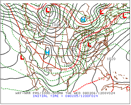
- What was the date and time the model was initialized?
- When was the prog valid (give time and date)? Briefly explain, incorporating the number of forecast hours associated with the numerical prediction.
- Here's an annotated version of the upper-right panel [2]. Notice Point P, which lies in the western Gulf of Mexico. Estimate the predicted surface wind direction at Point P (give your answer in degrees). Briefly explain how you arrived at your answer.
- Focus your attention on the low-pressure system predicted to be centered over the Ohio-Indiana border. Print the panel and then draw the cold and warm fronts associated with this low. Explain how you located the warm and cold fronts. Use your answer in part (c) to help you locate the cold front in the Gulf of Mexico.
- Is your placement of the cold front in the Gulf of Mexico consistent with the surface wind direction at Point P (from part (c)) and the precipitation pattern shown in the lower-right panel [3]? Briefly explain.
- Was the low-pressure sytem a mature mid-latitude cyclone at this forecast time? If so, confirm by printing the lower-left panel [4] and drawing the approximate axes of the low's cold- and dry-conveyor belts. Make sure you label each conveyor belt.
- What was the greatest downward motion that the WRF predicted in the immediate wake of the low or its cold front (at this forecast time)? Proper units and the sign (positive or negative) are a must! Where was the pocket of strong downward motion predicted to be at this forecast time? Did this predicted pocket of strong downward motion likely correspond to a specific feature associated with the mid-latitude cyclone? Please explain.
- In which state did the WRF predict the strongest cold air advection in the wake of the low's cold front (at this forecast time)? Explain your answer, incorporating the reason why you can use 1000-500 mb thickness contours as a proxy for isotherms.
- Estimate the predicted 1000-500 mb thickness at Buffalo, NY [5], at this forecast time. Units are a must!
- Notice that the WRF's lower-right panel [3] predicted precipitation to fall at Buffalo during the six-hour period ending the time the prog was valid. Using only the upper-right panel, what was the chance (greater than 50%, less than 50%, or equal to 50%) that the precipitation would fall as snow (versus rain) at Buffalo during the six-hour period ending the time the prog was valid? Explain your answer.
- Was your answer in Part (j) consistent with the meteogram for Buffalo (see below)? To justify your answer, cite specific type(s) of precipitation that fell during the six-hour period ending at the time the prog was valid.
Laboratory Exercise #2
The image below is the 12-hour forecast for mean sea-level isobars and 1000-500 mb thickness from the WRF run initialized at 12 UTC on February 7, 2008. For reference, here's the entire four-panel prog [6].
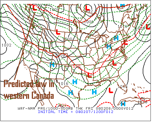
Note the low-pressure system predicted to be located in western Canada. Follow the movement and development of the low by running your cursor over the forecast times (see screen capture [7]) associated with the loop of progs of the WRF run initialized at 12 UTC on February 7, 2008 [8].
a. Based on the loop of WRF progs, what direction was the low predicted to move with time?
b. Keeping in mind your answer in part (a), what is the name given to this type of wintertime low-pressure system?
c. Focus your attention on the 48-hour forecast for mean sea-level isobars and 1000-500 mb thickness from the WRF run initialized at 12 UTC on February 7, 2008 (see below). For reference, here's the entire four-panel prog [9]. Print the 48-hour forecast for mean sea-level isobars and 1000-500 mb thickness [10] and draw the cold front associated with the low annotated on the 12-hour forecast above.
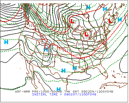
d. Explain how you positioned the cold front, based on the patterns of sea-level isobars and 1000-500 mb thickness.
e. Was this cold front an Arctic front (the leading edge of Arctic air)? Explain by pointing out a specific contour of 1000-500 mb thickess. Units are a must.
f. Now focus your attention on the WRF's 48-hour forecast for the six-hour liquid-equivalent precipitation (the lower right panel [11]). Based on the predicted position of the 850-mb isotherm corresponding to 0oC, what type of precipitation was likely to fall? Briefly explain your answer. Does the predicted position of the critical thickness support your answer? Briefly explain.
g. Based on the color-coded key for precipitation, what range in liquid precipitation does the WRF predict will fall in the six-hour period ending at 12 UTC on February 9, 2008? Units are a must.
h. Based on your answer in part (g), give a reasonable range for snowfall during the six-hour period ending at 12 UTC on February 9, 2008 (in the region annotated on the lower-right panel [11]). Explain your reasoning if you departed from the standard 10-to-1 ratio of solid to liquid precipitation.
i. Is such a range consistent with this type of wintertime low-pressure system? Please explain, incorporating the forward speed of the storm and its access to moisture.
Laboratory Exercise #3
This exercise asks you to apply what you've learned about numerical weather prediction to the cyclone model and the process of self development discussed in Chapter 13. You will work with 12-hour, 18-hour and 30-hour forecasts from the GFS run at 12 UTC on November 5, 2009. The map background for all the progs focuses on the western North Atlantic Ocean and eastern North America.
a. You are given the 18-hour forecast for 500 mb heights, winds, and absolute vorticity [12] (colors indicate relatively large values of absolute vorticity) from the 12 UTC GFS run on November 5, 2009 (valid at 06 UTC on November 6, 2009). Focus your attention on the prominent trough slated to move off the East Coast of the United States. In light of the corresponding 18-hour forecast [13] for mean sea-level pressure isobars, 850-mb temperatures, and precipitation for the six-hour period ending at 06 UTC on November 6, elaborate on the connection between the 500-mb trough and the relatively deep low-pressure system you observe at the surface. Please use references to specific longitudes and latitudes to describe the position of the low-pressure system with respect to the 500-mb trough.
b. Compare the 12-hour forecast [14] for mean sea-level pressure isobars, 850-mb temperatures, and precipitation for the six-hour period ending at 00 UTC on November 6 to the 18-hour forecast [13] in part (a). Was cyclogenesis [15] predicted to occur during this six-hour period? Please explain your answer.
c. You are given the 18-hour forecast [16] of 850-mb heights, isotherms (thin red and thin blue contours), and winds. What feature do you observe in the 850-mb heights in the immediate vicinity where the GFS predicted surface cyclogenesis to occur? What kind of temperature advection was this feature slated to generate south and west of the low-pressure system (east of the Carolinas)? Please explain your answer.
d. In light of your answer in part (c), what should happen to 500-mb heights with time in this area? Please explain in the context of the process of self development.
e. You are given the 30-hour forecast [17] for 500-mb heights, absolute vorticity, and winds (valid at 18 UTC on November 6). Does this prog support your answer in part (d)? Please explain, comparing specific values from the 18-hour 500-mb forecast [12] to this 30-hour 500-mb forecast.
f. Compare the 30-hour 500-mb forecast [17] to the 30-hour forecast [18] for mean sea-level pressure isobars, 850-mb temperatures, and precipitation for the six-hour period ending at 18 UTC on November 6. In what stage of development was this low-pressure system predicted to be at this time (that is, at 18 UTC on November 6)? Please explain.
Laboratory Exercise #4
On the afternoon of November 9, 2009, Tropical Storm Ida [19] bore down on the central Gulf Coast. By early morning on November 10, Ida was already on its way to becoming extratropical [20], a transition that wasn't surprising, given the inevitable cooling trend over land during late autumn and the corresponding seasonal increase in vertical wind shear. The 12 UTC surface analysis on November 10 [21] encapsulates the transition of Tropical Storm Ida to an extratropical low. Indeed, note the incipient front connected to the tropical-storm icon marking Ida's official position ... the "mixed" nature of this surface representation indicates that the developing system had both tropical and extratropical characteristics at this time.
The 12 UTC run of the GFS model on November 10 [22] predicted that the mid-latitude low-pressure system would become a memorable storm. To get a sense of the simulated evolution of the storm, run your cursor over the forecast times along the top of the progs. In case you're wondering, the labels, f06, f12, f18 and f24 (for example) correspond to the 6-hour, 12-hour,18-hour and 24-hour forecasts (respectively). Additionally, the individual progs associated with these specific forecast times were valid at 18 UTC on November 10, 00 UTC on November 11, 06 UTC on November 11, and 12 UTC on November 11 (respectively). In a nutshell, running your cursor over the forecast times allows you to look at a loop of progs so that you can get a sense of how the model predicts weather patterns and systems will evolve with time.
a. Focus your attention on the upper-left panel of the six-hour prog [23] (500-mb heights and 500-mb absolute vorticity). What kind of 500-mb feature did the GFS predict to lie above the extratropical remnants of Ida at 18 UTC on November 10? Briefly explain.
b. Slowly run your cursor over the forecast times between 6 and 48 hours [22]. Describe the interaction between the feature you identified in part (a) and a similar feature in the northern branch of the 500-mb westerly flow of air. Were these features predicted to eventually merge? Please explain. Recalling the general discussion in Chapter 16, what's the formal name that meteorologists give to this kind of interaction between the northern and southern branches of the 500-mb flow?
c. Focus your attention on the upper-right panel of the 48-hour prog [24]. At this forecast time, what was the predicted central pressure (approximately) of the mid-latitude surface low that absorbed the extratropical remnants of Ida? Proper units are a must!
d. Still referring to the 48-hour prog [24], qualitatively describe the magnitude of the predicted pressure gradient along the Middle Atlantic Seaboard (North Carolina to New Jersey) at this time. Was the mid-latitude surface low predicted to be exclusively responsible for this pressure gradient? Please explain.
e. Slowly run your cursor slowly over the forecast times after 48 hours [22]. For the Middle Atlantic States, was this expected to be a short-lived (less than 24 hours) or a more protracted [25] event? Please explain, specifically citing the evolution of the system on the upper-left and upper-right panels.
f. In addition to relatively strong and persistent winds, what other types of significant conditions should you have expected along the Middle Atlantic Coast? To help you formulate your thoughts, check out the following photographs taken along the Middle Atlantic Coast during the height of the storm. Photograph #1 [26] was taken at Wallops Island, Virginia, and Photograph #2 [27] was taken in Chincoteague, Virginia [28].
g. Write a short paragraph that relates the speed and persistence of the coastal winds to the threats documented in part (f). Please compose the paragraph in such a way that the general public will easily grasp the basic meteorology and oceanography of this event. Please include a general reference to the times of high astronomical tides.
h. In light of your answer in part (g), check out the satellite-derived rainfall [29] (in millimeters) from November 6-13, 2009. Over interior Virginia, what was the greatest rainfall? Express your answer in inches. Try this online converter [30]. What lifting mechanism likely contributed to the heavy rain over interior Virginia? Please explain.
Laboratory Exercise #5
MOS (pronounced "moss"), short for Model Ouput Statistics, is a statistical scheme that weather forecasters use to help them better predict surface temperatures, surface winds, and several other forecast parameters. MOS forecasts are typically presented in the form of a very compact table - here are instructions for interpreting NAM MOS (Description of the NAM MOS [31]) and GFS MOS (Description of the GFS MOS [32]) - you probably want to keep those descriptions open while doing this problem.
You are given the NAM MOS [33] and GFS MOS [34] for St. Louis, MO (KSTL), from the 12 UTC runs on December 6, 2009.
a. What were the high temperature forecasts from the GFS MOS and NAM MOS for December 7 and December 8? Provide a brief comparison.
b. What were the low temperature forecasts from the GFS MOS and NAM MOS for December 7 and December 8? Provide a brief comparison.
c. What were the NAM MOS and GFS MOS predicted temperatures for 21 UTC on December 8?
d. What were the NAM MOS and GFS MOS predicted wind direction and wind speed for 00 UTC on December 9? Express wind direction in both degrees and cardinal direction [35]. Proper units on wind speed are a must! Provide a brief comparison.
e. Give the time and date when the NAM MOS and GFS MOS predicted the lowest cloud ceilings. At what altitude were the ceilings predicted to be? Proper units are a must.
f. Referring to part (e), did the NAM MOS and/or the GFS MOS predict any obstructions to visibility? If so, provide the specific obstruction to visibility. Please explain, incorporating your answer in part (d) where it's appropriate.
Laboratory Exercise #6
This problem requires you to use the NAM MOS, GFS MOS and MOS consensus (the average of the two - see Laboratory Exercise #5 for the background material on MOS) to predict tonight's low temperature and tomorrow's high temperature for the town where you live (or the nearest city or town for which MOS data are available). Given the nature of this forecast, you should complete this assignment relatively early in the day - in other words, in the morning, afternoon, or early evening (waiting until the nighttime hours to complete this assignment essentially defeats the purpose of forecasting tonight's low temperature).
To do this exercise, follow these steps:
1. Go to the University of Wyoming's Web page for city forecasts and observations [36].
2. Pick the region or section of the country where your city or town is located.
3. Under MOS Forecasts, choose NAM MOS.
4. On the interactive map, scroll over the town/city in which you live (or the nearest town/city for which MOS data are available). The name of the city or town should appear. Click on the corresponding white dot. Copy and paste the pop-up MOS table into a Word file.
5. Repeat Step 4 for GFS MOS.
Based on the MOS data you just generated, answer the following questions.
a. What is the name of the city or town for which you generated the MOS data? What is its three-letter station identifier? For example, the three-letter station identifier for Allentown, PA, is ABE.
b. What were the time and date at which the NAM MOS and GFS MOS were initialized?
c. What are the NAM MOS and GFS MOS forecasts for tonight's low temperature? What is the MOS consensus? We define MOS consensus as the average of the NAM MOS and GFS MOS forecasts.
d. What are the NAM MOS and GFS MOS forecasts for tomorrow's high temperature? What is the MOS consensus?
e. To do this final part of the question, you need to wait until the day after tomorrow to verify your forecast. To verify your forecast, follow these steps:
- Go to the interactive map of the National Weather Service Forecast Offices [37]. Click on the forecast office closest to the town or city in which you live.
- You should see a link labeled "Climate and Past Weather." Click on that link.
- At this point, you want to generate the Daily Climate Report for the day you made your forecast. Daily Climate Report is the default setting on the Local Climate Page, so there's nothing for you to choose in the Product menu (on the left). Make sure your city or town is highlighted in the Location menu (in the middle). If your town does not appear in the menu, select the nearest city or town, but please try your best to make sure the town/city for the MOS data you generated and the Daily Climate Report are for the same city or town. In the Timeframe menu, Most Recent is the appropriate choice if yesterday was the day for which your forecast applied. If you waited longer, select Archived Data and choose the appropriate date (the date for which your forecast applied).
- Copy the Daily Climate Report and paste it into a Word file. What were the verifications for the high and low temperatures? Write a paragraph that describes how NAM MOS, GFS MOS, and MOS consensus performed.