Module 1: Past Episodes of Climate Change
Module 1: Past Episodes of Climate Change
Video: Earth 103 Quarry Module (1:10)
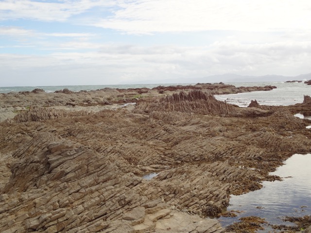
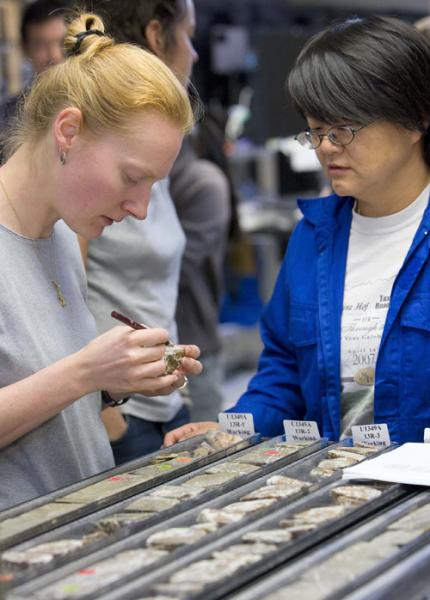
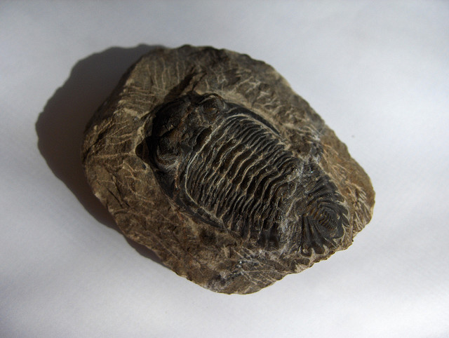
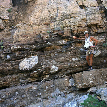
Good morning, we've just crossed an important threshold in Earth history. Global CO2 concentrations now are above 400 parts per million. That is really significant because, as we'll learn a lot about in this class, CO2 is a very potent greenhouse gas and it's responsible for the warming and climate that we're seeing. Now, you have to go back many millions of years to find CO2 concentrations in the atmosphere as high as they are today. It is really critical to understand what happened in Earth's past because it can inform us about what's going to happen in the future. Now, I'm standing here in a quarry in rural Pennsylvania and these rocks behind me were deposited in a shallow ocean about 450 million years ago, and geologists have worked really hard to establish chemicals and fossils that can tell us about conditions in the past. So, by studying the chemicals and fossils in rocks such as these, we can learn what's in store for the future of the Earth.
Introduction
The geologic record is an incredibly detailed archive of Earth's history. Visit the Library of Congress and you can find out any information on the history of the United States of America. Only a very small part of the history of the Earth has been recorded by humans. Much of the history is, in fact, contained within naturally-formed, geologic materials. Sample sedimentary rock sequences and ice cores, and you can glean an incredibly detailed record of Earth's climate, environment, and life history. Earth's history book goes back over four billion years, but interpreting this history is not nearly as simple as reading the history of our nation. The Earth's book has been buried under hundreds and thousands of meters of rock and ice and that has altered the signals that geologists use to reconstruct climate, environment, and life history. Imagine a history book that has been burned, soaked, and torn apart many times, and you might then understand the difficulty geologists have interpreting the history of the Earth.
Over the last century, geologists have made remarkable progress unraveling Earth's history, and what an amazing record it is! As we will learn in this module, we now know that there are times in the past when palm trees grew on the shores of Alaska and on the plains of Wyoming, and when reptiles colonized the islands of northern Canada. There are other times when ice sheets apparently encircled the entire globe and, more recently, when an armada of giant icebergs swept off Canada and Greenland and covered large swaths of the Atlantic Ocean. Crucially, for today’s climate the geological record tells us that Earth has not been as warm as it is today for 125,000 years!.
We will learn in this class that climate and environmental change is threatening modern ecosystems, and that this threat will increase substantially in the future. But Earth history informs us that there are times in the past when 90% of species in the ocean were eradicated during mass extinction events, but the remaining 10% were able to survive, and, in fact, take advantage of the open niche space. Life in the past was extraordinarily resilient to some of the harshest environmental changes one can imagine. For example, the asteroid impact that wiped out the dinosaurs 65 million years ago caused large wildfires, followed by weeks or months of nearly complete darkness, and highly acidic and possibly toxic oceans. Yet, life hung on by a thread. If life could survive that level of harshness, then why are many ecosystems today in such distress? This is a central question of modern ecology, and something we will explore in great detail later in the course.
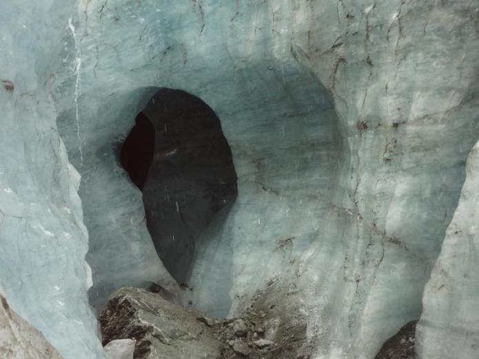
But let's start by discussing how Earth's great historical archive is recorded. As we will see shortly, the archive is actually built from a number of materials besides sediments and ice. Corals, stalactites formed in caves, and trees also carry signals of the environmental conditions when they were living or were formed. But here, we will focus on sediments and ice that carry the majority of the historical record.
The sediment archive covers the entire record of the Earth. In fact, the archive holds the majority of the history, especially in what geologists call “deep time”, before the last million years or two. Sediments are deposited in a wide range of environments including lakes, rivers, deserts, and the ocean all the way from the beach to the deep sea. These sediments contain a range of different particles, depending on where their material derives from. Sediments formed on land are largely made of what is known as clastic materials, minerals derived from the weathering of rocks. Some of these environments such as lakes also contain the fossilized remains of living organisms. Marine sediments, especially those that were laid down in the deep ocean, are largely composed of these fossils. Sediments are deposited by water, wind, and ice, in a “layer cake” fashion, with the older layers underlying the newer layers. Each layer represents a unique period in Earth’s history and preserves the environmental snapshot of that time interval. One of the main challenges with this record is determining how old individual layers are. To do this, geologists use a combination of the fossils in the layers, the orientation of magnetic grains, as well as minerals that contain radioactive decay products such as carbon-14 and lead. However, with a great deal of intensive and laborious work, geologists have provided the age control that enables the interpretation of a truly remarkable record of Earth’s climate environment and life history.
On top of glaciers in places such as Greenland and Antarctica, but also in mountainous regions, snowfall accumulates layer upon layer in much the same way as marine sediment. As this snow is buried by other layers, it is gradually compacted to form ice. Ice accumulates extremely consistently, and annual layering is usually very apparent, so obtaining age control in ice is much simpler than dating sediments. In addition, ice can be dated using carbon-14 as well as very thin layers of material called ash that derives from volcanic eruptions.
So, now, down to the brass tacks. How is information on climate obtained? This is yet another really detailed and impressive story.
Goals and Learning Outcomes
Goals and Learning Outcomes
Goals
On completing this module, students are expected to be able to:
- explain how sediments, ice cores, and tree rings record geological time;
- explain how proxy information on past climates is extracted from geological materials;
- infer the nature of climate change from proxy records;
- consider how ancient events can inform us of changes to come in the future.
Learning Outcomes
After completing this module, students should be able to answer the following questions (hint: each of these topics is the subject of one quiz question!):
- In what materials is evidence of ancient geologic environment recorded?
- What is the "Hockey Stick"?
- What gases do ice bubbles contain?
- What is a piston corer?
- What are the processes that fractionate oxygen and carbon isotopes?
- What are the other proxies for temperature?
- How do tree rings record climate?
- What are foraminifera?
- What are the characteristics of leaves from tropical environments?
- What is moraine?
- What are the changes that occurred during glacial-interglacial cycles?
- How was the PETM initiated and what happened during the event?
- What was the impact of global warming during the PETM on life?
Assignments Roadmap
Assignments Roadmap
Below is an overview of your assignments for this module. The list is intended to prepare you for the module and help you to plan your time.
| Assignment | Location | |
|---|---|---|
| To Do |
|
|
Climate Records
Climate Records
Google the words “hockey stick,” and in addition to advertisements for sporting equipment, you will find links to one of the most chronicled and scrutinized datasets in modern science, the climate record of the last millennium. The curve was originally documented in a paper authored by Penn State Meteorology and Geoscience Professor Michael Mann and his colleagues. As shown in the figure below, the curve shows fairly constant temperatures or even a modest cooling from 1000 to about 1900 AD. About 1900, a sharp warming trend began, the base of the hockey stick. This warming has continued almost unabated to the present day. It so happens that the base of the stick corresponds to later stages of the industrial revolution, a time when the release of greenhouse gases from fossil fuels to the atmosphere spiked. The correlation of warming and the increase in levels of greenhouse gases, which are known to trap heat in the Earth’s atmosphere, is hard to argue with.
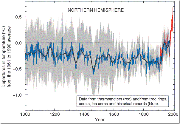
Perhaps the most scrutinized aspect of the hockey stick graph, and where the scientific controversy has focused, is that a part of the data set derives from temperature measurements that have been made since about 1900. The remainder of the curve derives from historical records and "proxy" measurements that are made indirectly. "Proxies" are substitute measurements that are made to determine the conditions at times before humans could measure climate directly. Such proxies serve as the basis for our understanding of past climate. In this module, we will learn how proxy measurements are made.
Fortunately, the history of the earth, including the evolution of its physical environment and its life forms, is beautifully preserved by a variety of Earth processes. For example, as we discussed briefly on the last page, sediments deposited in the ocean basins accumulate in a layer-cake fashion and entrap the fossil remains of once-living organisms. In addition, when these organisms, including species of clams and corals, were living, they recorded Earth’s climate history in the chemistry of layer upon layer of their shell. Images of a layered clamshell and coral skeleton are shown below.
Samples of Climate Records
Video: Sedimentation (1:02)
There are three different sources of sediment to the deep sea sedimentary record. The first is terrigenous material that is delivered via rivers into the oceans. The second is dust that is blown in from the continents by winds. And the third is biogenic material, formed by organisms that lived on the surface of the ocean that died and then subsequently rained down through the water column to the seafloor. Regardless of source, these types of material are buried in the deep sea sedimentary record. The nature of the sedimentation process is such that the youngest material lies close to the sea floor, and as the sediment becomes progressively deeper, it becomes progressively older. Thus, the deep sea sedimentary record provides a beautiful inventory of ancient climate from younger to older.
As we will detail below, chemical proxies allow the climate to be reconstructed from shell materials many hundreds of millions of years old. In fact, some of the best records of Earth’s climate are obtained from mile upon mile...., sorry kilometer upon kilometer, of cores removed from the ocean floor. The current ocean basins are less than 180 million years old, meaning that only the last 180 million years of Earth’s history are preserved in the current ocean. Fortunately, large-scale Earth tectonic processes have elevated vast piles of sedimentary rocks onto the land, where they are preserved in mountains and elsewhere. These materials can be sampled in road cuts and cores and climate information gleaned from them, taking our understanding of climate history much further back.
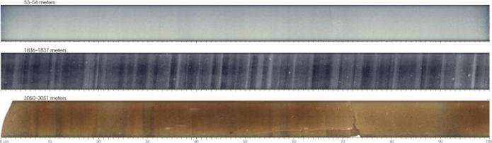
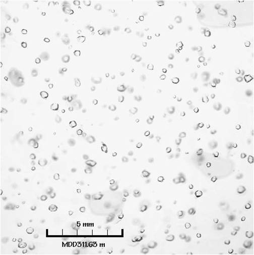
The major ice sheets have accumulated layer by layer over time. These layers record temperature, precipitation, and wind patterns at the time the ice formed. Tiny gas bubbles trapped within the ice preserve the composition of the atmosphere including levels of CO2 and methane (CH4). Kilometer upon kilometer of cored ice and the bubbles within it preserve an incredible record of Earth's climate variations for hundreds of thousands of years. See the images shown below of the GISP2 Ice Core and a sample of atmospheric gas bubbles in ice.
Video: Ice Accumulation (1:34)
Ice cores provide valuable inventories of ancient climate. This slide here shows various levels of the ice core, illustrating how the physical properties of ice change from the surface down to the bottom. Ice formed from snow that was precipitated on the top of the glacier. The uppermost panel shows the properties of snow, very loosely compacted, showing the few annual layers that we'll describe later on, in the snow, and very small trapped bubbles of air. In the middle panel, from deeper within the glacier, approximately 1838 meters down, the ice is more compacted and shows a very strong annual banding with darker layers indicating slow accumulation rates of ice during the warmer months, and lighter layers showing the rapid accumulation of ice during the winter months. In this layer, you can see, nicely trapped bubbles of gas. Close to the bottom of the glacier, where erosion of the underlying bedrock is common, the glacier has a dirty color, a brown color, because of the content of eroded minerals and rock particles in the ice. This here shows the glacier close to the base, at about 3000 meters below the surface.
The accumulating ice also preserves dust, smoke, pollen, and ash from volcanic eruptions. The texture of summer snow and winter snow is very different, and the resulting layers provide very accurate means to determine the age of ice cores, as does C-14 dating of the CO2 trapped in ice bubbles. In this way, the composition of the atmosphere can be determined hundreds of thousands of years back in the past. Imagine this, the air that your great-great-great-great grandparents breathed has been collected in some lab around the world!
Check Your Understanding
Climate Question
Climate Records: Sampling
Climate Records: Sampling
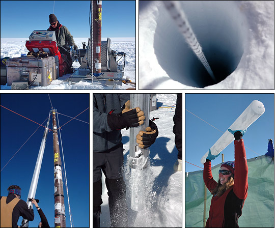
Sections of ocean sediments have been sampled extensively by a suite of coring operations dating back to the 1940s. These operations include a variety of different drill ships as well as rigs like the ones that are used in oil exploration. In all cases, the retrieval of continuous cores from the seafloor requires a drill string, a continuous line of pipe that is assembled to extend from the ship or platform to the seafloor.
Once the drill string reaches the seafloor, a metal core barrel is lowered through the pipe to recover sediment. Typically, each core that is extracted is between 2 and 10 m long. At the head of the core barrel, is the bottom hole assembly, a device that is positioned to cut the core. A variety of different techniques are used to cut sediment. Where the sediment is young and soft, as occurs in younger layers close to the seafloor, cores can be cut using a piston-coring device (see figure below). The piston is situated inside the core, and it is triggered when the bottom hole assembly is close to the ocean bottom. When it hits the bottom, the piston rapidly moves up, so the mud fills the empty pipe as it sinks. At the end of the bottom hole assembly is a drill bit that actually helps cut through the core. In the case of the piston core, the bit is a sharp, knife-like device that helps the rapidly advancing core cut readily through the soupy sediment. If the formation is harder, as occurs deeper in the sediment column where the overlying burial has led to compaction and cementation, cores can only be retrieved using a hard bit that cuts the rock by rotating at high speeds assisted by water, and, in some cases, drilling mud (this is known as rotary coring). Compared to the piston core which advances in seconds or less, this rotary coring can take a very long time, often up to an hour for each meter of core; moreover, some of the sediment can be lost during coring, as pressure from water or mud must be applied to cut through the rock. Once the coring mechanism is fully extended, a core catcher slips into place underneath the coring device and a wire line is used to retrieve the core to the ship or drilling platform.

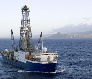
Probably the best-known and longest-running drilling operation, the Integrated Ocean Drilling Program (IODP) has been in operation for more than 40 years. The program began as the Deep Sea Drilling Project in 1969 and is a collaborative scientific operation between a number of different countries. The ship chartered by the program is the JOIDES Resolution, a highly sophisticated drilling platform that has the ability to take cores in locations where the ocean is 6000 meters deep. The ship is about 150 meters long, with a drilling derrick that is about 50 meters high. The deepest hole drilled by IODP exceeds 2000 meters. The ship can operate in stormy seas with large waves and strong currents as it is held in position by powerful turbines, and the drill pipe is stabilized by a device called a heave compensator that keeps the drill bit on target even when the ship is listing. The Resolution has berths for about 120 engineers, scientists, drilling “rough necks,” and caterers, and typically stays out to sea for six- to eight-week expeditions.
As we will see below, valuable information about Earth’s climate has been obtained by drilling in the ocean basins. However, rocks that were deposited in continental environments and marine sediments that have been uplifted onto the continents via plate tectonics also provide important information about past climates. These rocks are much more readily accessible and can be sampled in road cuts, stream beds, and many other places. In addition, sedimentary rocks on land can be sampled via coring with much less expense than their oceanic counterparts.
Samples of land materials are often taken by digging a trench to obtain fresher material beneath the weathered surface zone. If the material is indurated, samples of core are removed using a saw and samples of outcrop are removed using a hammer. Soft material usually in cores can be sampled by inserting plastic tubes into the sediment. Once the samples are taken, the material is ready for analysis.
Over the long term, cores of sediment are usually kept in refrigerators to keep them from drying out. Cores of ice are housed in warehouse-sized refrigerators that are cooled to -30oC. The longest ice core sampled is the three-kilometer long Dome C core from Antarctica that extends back some 750,000 years.
The following video provides an excellent overview of how cores are collected by the Integrated Ocean Drilling Program. Click the play button in the center of the video to watch it.
Video: Core on Deck!: The Journey of how the Samples travel from the Rig Floor to the Core Lab (7:26)
Text on screen: Exploration, Discovery, Understanding. Integrated Ocean Drilling Program. Understanding Earth History via Scientific Ocean Drilling. Part One: Collecting and Processing Sediment Cores.
Hi, my name is Tim Brock. I'm an assistant lab officer on the Joides Resolution. My job here is to supervise a group of marine lab specialists and to ensure that the core that we've brought up is processed in a timely manner and accurate manner. Joides Resolution or the JR, as we call her, is 470 feet long 70 feet wide and can drill in 29,000 feet or 8800 meters of water. The Joides Resolution and the research it supports make up the integrated ocean drilling program. It all began with the Mohole project in the 1950s and that showed deep-ocean drilling to be a viable means of obtaining geological samples. Ocean drilling has the advantage in that the samples are undisturbed from atmospheric and surface conditions, and that provides a better geological record. The sediment and the hard rock that we harvest are in the form of cores, and locked within them is no less than the history of our planet. Each expedition has been carefully chosen by an international group of scientists, for its scientific value and its location. They are currently exploring the Bering Sea and its unique formations which lie underneath its waters. Harvesting the core is an immensely complex process. I'm standing on the core receiving platform, or the catwalk, as we call it, and I'm here to explain one small part of the process: how the core gets from the rig floor to the core receiving platform, to the core laboratories. Voice over a loudspeaker: On deck, grande. Those words announce the arrival of the core barrel from its long journey from the seafloor. Contained inside are answers to the questions which the scientists seek. The cutting shoe is removed from the end of the core barrel. It contains a core catcher which secures the sediment-filled core liner inside. The core catcher is taken to a bench to be disassembled. Next, the liner is removed. The 10 meters of core is carried to the core receiving platform. The technicians must work quickly, as another coring tool is already on its way down to the seafloor. There is only a limited amount of time. The core liner must be cleaned, cut, curated, engraved, and labeled before the next core hits the rig floor. The core is measured, to be cut into 150-centimeter sections. A specialized cutting tool is used to cut the core liner. Now, the core is more easily handled. Here, a microbiologist cuts the core with a sterilized spatula and take small plugs of sediment. This sediment will be tested for the presence of microbes living at extreme environmental limits. A sample of sediment is given to a paleontologist. Microfossils found within are used to determine the age of the sediment. The remaining sediment is carefully repackaged into a section of core liner. The core liner section is sealed with colored end caps, indicating the orientation of the core. Acetone is applied to the end cap and seals the cap to the liner by chemically melting the plastic. At last, the sections are taken into the core lab. Each section has its unique core number and section number engraved into the core liner, and a barcode label attached. So, there you have it. The ship never sleeps. We drill 24 hours a day, seven days a week. This happens hundreds of times over a normal two-month expedition. Thanks for your time. I've got to get to work.
Proxy Techniques: Stable Isotopes, Trace Elements and Biomarkers
Proxy Techniques: Stable Isotopes, Trace Elements and Biomarkers
Oxygen Isotopes
Since we cannot travel back in time to measure temperatures and other environmental conditions, we must rely on proxies for these conditions locked up in ancient geological materials.
The most widely applied proxy in studying past climate change are the isotopes of the element oxygen. Isotopes refer to different elemental atomic configurations that have a variable number of neutrons (neutrally charged particles) but the same number of protons (positive charges) and electrons (negative charges). As you might remember from your chemistry classes, protons and neutrons have equivalent masses, whereas electrons are weightless. So, because different isotopes of the same element have different weights, they behave differently in nature.
Oxygen has three different isotopes: oxygen 16, oxygen 17 and oxygen 18. These isotopes are all stable (meaning they do not decay radioactively). O-16 is by far the most common isotope in nature, accounting for more than 99.8% of all oxygen atoms, and O-17 is exceedingly rare, but O-18 is abundant enough in nature to be measured. The masses of O-16 and O-18 are different enough that these isotopes are effectively separated by natural processes. This separation process is known as fractionation. Without going into too much detail, O-16 and O-18 are fractionated by the process of evaporation as well as when minerals, including shells of animals and plants, are precipitated from water. The main driver of the evaporation effect in most geological intervals is the amount of water that has been removed from the ocean and is sequestered in ice (see video clips below). Evaporation selectively removes the lighter isotope, O-16 from water leaving higher concentrations of the heavier isotope, O-18. Thus, shells and other materials formed in the ocean tend to have more O-18 during colder, glacial intervals than during warmer intervals. However, as a portion of the evaporate ends up falling as snow which is then converted to ice, the reverse holds for ice sheets, such as those in Greenland and Antarctica. Ice formed in glacial intervals has more O-16 than ice grown in warmer times. Superimposed on the evaporation effect is a temperature effect. Shells that grow in warmer water hold more O-16 than shells that grow in colder water, as explained in the following clips:
Video: Stable Isotopes 1 (1:34)
Oxygen has three major isotopes: oxygen 16, oxygen 17, and oxygen 18. All of these isotopes have eight protons, but oxygen 16 also has eight neutrons. Oxygen 17 has nine neutrons, and oxygen 18 has 10 neutrons. Because these substances have different weights, they behave differently in nature, and this allows environmental processes to fractionate them. By fractionation, I mean separation of the various I States by natural processes. And this fractionation allows geologists to use the isotopes as proxies. Here we consider the temperature proxy of oxygen isotopes. Oxygen 16 is much more abundant in nature than oxygen 18, but its mass provides for mass-dependent fractionation from oxygen 18. And this is a result of vibrational frequency differences that operate at different temperatures. For example, in the formation of calcite (CaCo3), warmer water will lead to the inclusion of more oxygen 16 in the calcite molecule. In colder water, more oxygen 18 will be included in the calcite molecule. This allows us to use the relative ratio of oxygen 16 and oxygen 18 in the calcite of foraminifera as a proxy for paleo temperature.
Video: Stable Isotopes 2 (1:42)
The second way in which oxygen isotopes are fractionated is via kinetic processes, for example, evaporation. Evaporation acts on oxygen isotopes because the light isotope of oxygen, oxygen-16, is more readily evaporated from water than oxygen-18. Thus, clouds contain more oxygen-16 than oxygen-18. And the rainfall that comes from these clouds also contains more oxygen-16 than oxygen-18, as does the snow that forms from the rain. When you have a warm climate without snow, most of this oxygen-16 that is included in these clouds evaporates, precipitates, and is returned to the oceans. When you have a cold climate, most of the oxygen-16 becomes locked up in ice. And therefore, the water, the seawater from which this evaporation ultimately drives, becomes more enriched in oxygen-18. Thus, when we have calcite--foraminiferal calcite-- that forms from seawater, in a cold climate, the foraminifera will tend to be enriched in oxygen-18. Whereas, in a warm climate, the foraminifera will tend to be enriched in oxygen-16. Likewise, when we have snow and ice forming in a cold climate, it will tend to be enriched in oxygen-16. Whereas, when we have a little bit of snow or ice forming in a warm climate, it will tend to be more enriched in oxygen-18.
A range of materials from the geological record demonstrates significant variations in their levels of O-16 and O-18 as a result of changes in climate. These changes are a combination of temperature and evaporation effects. The materials include shells of clams, corals, and plankton called foraminifera that inhabit the surface of the ocean, as well as cores taken from glacial ice that has formed at high latitudes (a term that describes the cooler regions closer to the poles) and high elevations, and even stalactites formed in caves. Later in this module, we will study the isotope records of several intervals of rapid climate change in the geological record.
Other temperature proxies: Mg/Ca and TEX-86
As we have seen, there are a number of assumptions that need to be made to convert oxygen isotope values to temperature. At times when there were major ice sheets, the proxy can be difficult to apply and in fact, most applications of oxygen isotopes during cold intervals focus on changes in ice volume, not warming or cooling. Thus, it is fortunate that there are other proxies that can be applied to determine temperature. Here, we consider two of these, the ratio of magnesium to calcium in fossil CaCO3 shells and the TEX-86 ratio in organic carbon.
Mg/Ca
Organisms that construct shells of the two CaCO3 polymorphs, aragonite and calcite, include magnesium in very small amounts in their shells. As it turns out that amount is heavily dependent on temperature as a result of somewhat complex kinetic processes. The higher the temperature, the more Mg is included in the shell. Unfortunately, there are a few complications that need to be considered. Like oxygen isotopes, the Mg/Ca proxy requires that all of the calcite or aragonite is original and that it has not been altered during burial of the shell. Second, the ratios appear to differ from one species to another, thus there have to be careful calibrations for individual species. These calibrations focus on developing a relationship between the Mg/Ca of the shell and the temperature of the water in which it grew. This can only be done in living obviously. For extinct species, assumptions need to be made and they result in some uncertainty. Workers are careful to restrict their Mg/Ca analysis to individual species. Third, the Mg/Ca ratio of seawater has changed slowly over time and this ratio can impact the absolute temperatures when the focus of study extends over many millions of years. The proxy is most useful when the study interval is short, the fossil shells are unaltered and the species are still living. Since Mg/Ca is not impacted by the volume of ice as are oxygen isotopes, the proxy is often used along with the latter system to determine the volume of glaciers in cold geologic period.
TEX-86
TEX-86 is a complex organic (meaning material that is composed largely of carbon, nitrogen, and phosphorus) proxy. This proxy is applied to compounds made by archaea or single-celled prokaryotes (organisms that do not have a differentiated nucleus). The archaea in question live in the oceans and are called crenarchaeota, and the TEX-86 proxy is based on changes in the composition of the lipid membranes of these organisms. The detailed structure of the membrane changes with temperature. The proxy is called TEX-86 because it is based on the tetraether index in carbon-86 atoms (you do not need to remember this!). TEX-86 has been calibrated in the modern oceans, meaning the indices of samples have been compared to the temperatures of the water in which they grow. The main uncertainty of the system revolves around the fact that the organisms of interest do not live right on the ocean surface so the temperatures theoretically are lower than surface levels. In addition, it appears that the index is impacted by the growth rate of the organism. Application of the TEX-86 is restricted to marine sediments and is most useful where there are no shells to measure for oxygen isotopes or Mg/Ca. Regardless of the uncertainties, the TEX-86 proxy is extremely useful to check results from these other two systems. Where two different proxies agree for the temperature of an interval the results are much more certain.
Carbon Isotopes
Oxygen is not the only abundant element with isotopes that can be used as environmental proxies. The isotopes of the element carbon also are used as proxies in environmental reconstruction. Carbon has a number of isotopes including C-14, which is radioactive, and two stable (i.e. non-radioactive) isotopes, C12 and C13. C-14 are widely applied in dating recently formed natural materials that contain significant amounts of carbon such as shells, charcoal, and even materials that contain trace amounts of carbon such as pots and cloth, since its abundance can be accurately determined using an accelerator, and its rate of decay is rapid.
Video: Stable Isotopes 3 (1:40)
The three main isotopes of carbon are carbon-12, carbon-13, and carbon-14. Carbon-12 has six protons and six neutrons, carbon-13 has six protons and seven neutrons, and carbon-14 has six protons and eight neutrons. Carbon-14 is a radioactive isotope and disappears after a hundred thousand years. In addition, carbon-12 is much more abundant in nature than carbon 13. Because Carbon-12 and carbon-14 have different atomic weights, these isotopes are fractionated via a number of different biological processes. The main process that fractionates carbon-12 in nature is photosynthesis. Because carbon-12 is much lighter than carbon-13, the organic material formed via photosynthesis is enriched in carbon 12, and the material from which this organic material forms, the atmosphere or the ocean, remains enriched in the other isotope, carbon-13. Other processes that fractionate carbon-12 and carbon-13 include respiration and the formation of methane. Because biological processes operate over time and fractionate carbon-12 and carbon-13, the ratios of carbon-12 and carbon-13 in natural materials is changed significantly over time and this fractionation has a number of different applications, as we will see later in the module.
However, because of its rapid decay, C-14 disappears in a short time (about 100,000 years). The isotopes C-12 and C-13 are not radioactive, are common in natural materials, and are fractionated by environmental processes in a way that they can be applied as proxies. C-12 has 6 protons and 6 neutrons and is the most abundant of all of the isotopes of carbon. C-13 has 6 protons and 7 neutrons and is much less abundant than C-12, but still can be measured by mass spectrometry (the technique used to measure the abundance of stable isotopes). C-12 and C13 are strongly fractionated during photosynthesis when plants convert CO2 and sunlight into food; it requires less energy for a plant to incorporate an atom of the lighter isotope C-12 than it does an atom of C-13. In fact, when plant material is formed via photosynthesis, thousands of times more C-12 is incorporated than is C-13. As we will see, carbon isotopes are key indicators of the sources of greenhouse gas in the atmosphere both today and in the past. C isotopes can be used as proxies for nutrient cycling and deep water circulation as well as the source of plant materials.
Check Your Understanding
Oxygen Isotope Question
Proxy Techniques: Fossils and Rocks
Proxy Techniques: Fossils and Rocks
Tree Rings
Tree rings have been widely applied in climate reconstruction. Rings are produced as a result of seasonal variations in the growth rate of tree bark. Wood produced during rapid growth, for example in spring in temperate regions, tends to be less dense than wood produced during slower growth phases during the late summer and early autumn. Where seasonal growth is highly variable as in temperate regions, rings are strongly etched in the bark.
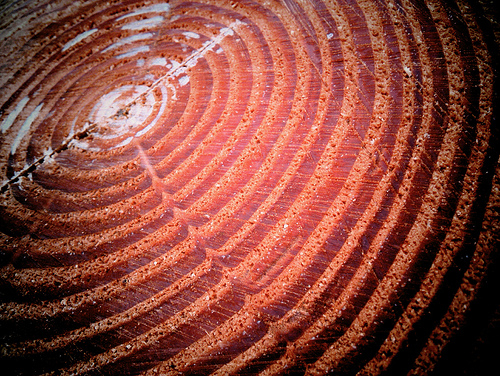
As shown in the image above, tree rings are especially powerful paleo climate indicators because the number of rings can be counted to determine the age of the tree or the age of the ring that is providing paleoclimate information. The width of tree rings can be interpreted in terms of temperature and precipitation variations; however, there are a number of factors that complicate this interpretation.
Video: Tree Rings Explained (1:54)
Tree rings preserve an amazing inventory of Earth's climate. This photograph shows a section through part of a tree, a living tree, and it contains dozens of tree rings. An individual ring consists of a lighter part and a darker part. The lighter part is preserved, or grown, during the rapid growth season in late spring and early summer, whereas the darker part, which is made of denser wood, hence its darker color, is grown, or preserved during the latter part of the summer and the fall. Combined, the light and the dark layer preserve one annual growth cycle of the tree. Therefore, the number of rings can be counted to provide an estimate of the age of the tree. Additionally, the thickness of the ring gives us a measure of the suitability for the growth of that tree at that time. So a thicker combination of light and dark indicates good growing conditions, such as warm temperatures and high rainfall, whereas thin rings indicate poorer growing conditions, such as colder conditions and a lower rainfall, or more arid conditions. Sometimes a tree doesn't grow at all during the year, in which case, the ring isn't preserved at all for that time period, and this would complicate using the number of rings for dating the tree. In temperate regions, tree rings are very well-preserved because the growth changes from summer to winter, whereas in tropical regions, rings are not as well-preserved because the tree is growing pretty well continuously.
Fossils
Fossils represent the remains of life that once thrived in the oceans or on land. They range in size from dinosaurs to shells of clams and oysters, all the way down to microscopic remains of algae, fractions of a millimeter in size. Although many groups of fossils can yield information on climate and environment, in this module we focus on the fossil remains of plants as well as those of the microplankton and microbenthos. These microfossils include a number of key groups that live in the ocean and in freshwater bodies such as lakes.
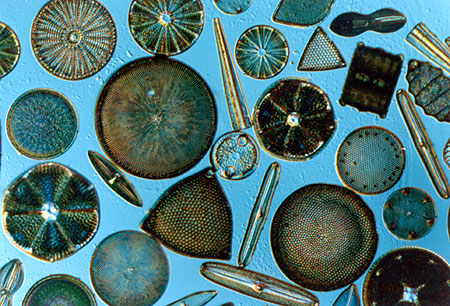
Diatoms
The diatoms are a group of plankton that makes their shell out of opal (microcrystalline SiO2). These organisms are autotrophic, meaning they fix CO2 dissolved in seawater or lake water via photosynthesis. The delicate diatom shell, or frustule, consists of two valves that fit together like a pillbox. The diatom cell lives inside the frustule and the plastids or chloroplasts use light as a source of energy in photosynthesis. Diatoms thrive where nutrient and silica levels are high: in lakes, the coastal ocean, and in the Southern Ocean, the ocean that circles the globe just north of Antarctica. Diatoms reproduce asexually (vegetatively), and, where conditions are right and nutrient levels elevated, diatoms can rapidly produce cell counts of many millions of cells per liter of seawater. In certain cases, as we will see in Module 7, these count levels are called red tides, and in some of these cases, diatoms produce toxins.
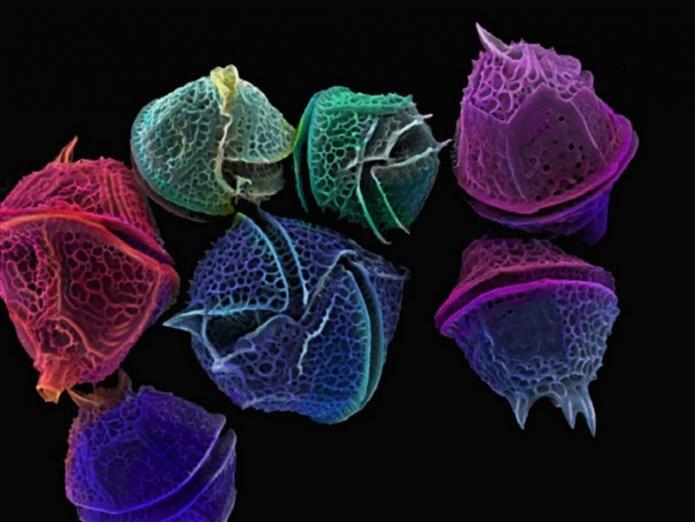
Dinoflagellates
The dinoflagellates are a group of plankton that is mostly autotrophic but can also be heterotrophic. The dinoflagellates thrive in the coastal ocean and have a complex life cycle in which a floating, motile stage alternates with a dormant resting stage. The dinoflagellates make their tests out of cellulose, which is rarely preserved; however, the cyst stage of dinoflagellates is composed of sporopollenin, a polymer that preserves readily during burial. The dinoflagellates are the group primarily responsible for red tides; we will discuss them in detail in Module 7.
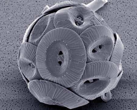
Coccolithophores
The coccolithophores, like the diatoms and dinoflagellates, are a group of marine autotrophic plankton. The coccolithophores, however, make their delicate shell out of the mineral calcite, or CaCO3, and have a more ocean-wide distribution than the diatoms. Today, the coccolithophores are adapted to live where the diatoms and dinoflagellates cannot, in parts of the ocean where nutrient levels are lower. Like the other groups, the coccolithophores are able to produce extremely large numbers of cells per liter in so-called blooms. Unlike the other two groups, the coccolithophores are threatened by ocean acidification, as we will see in Module 7.
Pictures of Foraminifera and Coccolithophores
Foraminifera
The foraminifera are zooplankton, meaning they consume tiny phytoplankton to get their energy. The foraminifera, or forams as they are known, make their shell out of calcite or CaCO3. The delicate foram shells have a variety of shapes and are adapted to the life mode of the individual species. The forams have two very different modes of life. The planktonic forams float passively in the water column, whereas the benthic forams live on the seabed, either resting on the bottom or burrowing into the soft sediment. The foraminifera have been critical in the reconstruction of ancient ocean temperatures via stable isotopes and trace element proxies, as we will see below.
The following video provides an overview of the foraminifera.
Video: Fossils and Rocks (2:10)
The foraminifera are a group of planktonic and benthic protists. That means they are single-celled organisms that float on the surface of the oceans or sit on the bottom of the oceans and live there. Foraminifera make their shells out of the mineral calcite (CaCo3). Planktonic foraminifera have a shell that's adapted to be buoyant in the water. Whereas benthic foraminifera have a shell that's adapted to either rest on the bottom of the ocean or burrow in the sediment. This photograph shows a planktonic foraminifera, which has a chambered shell. Individual chambers are formed and they rotate, with the outermost chamber being the chamber in which the organism inhabits. The foraminifera extends protoplasm from its outermost chamber and this protoplasm is used to grab its prey, specifically other protists, including the coccolithophores, diatoms, and dinoflagellates. At the same time, the protoplasm actually holds zooxanthellae, which are dinoflagellates that live in a symbiotic relationship with the planktonic foraminifera. The dinoflagellates help in the calcification of the foraminiferal shell. Benthic foraminifera live on the bottom of the ocean and they have a very strong application in providing depth information about the ancient sediments in which they're living. They also tell us about the oxygen supply on the bottom and the amount of food that's delivered through the water column. Planktonic foraminifera are most widely used in reconstructing paleo temperatures. Their shells also tell us a lot about geologic time as their shell morphology has evolved through the course of geological history.
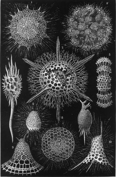
Radiolaria
The radiolaria are zooplankton like the foraminifera. The radiolaria are one of the longest-lived plankton groups, extending back to the early part of the Cambrian period about 500 million years before present. The group makes a spaceship-like test out of opal (SiO2) and, like the diatoms, is restricted to places in the ocean where nutrient levels are elevated. The radiolaria thrive in the tropical regions where upwelling currents bring nutrients to the surface ocean.
Plant Fossils
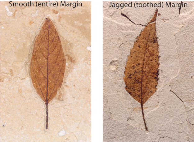
Plant fossils have been widely used in paleoclimate studies. These studies are based firmly on the distribution of modern plant species and on physical characteristics of those plants that are related to climate. The distribution of tropical plant species such as palms, cycads or groups of ferns can be used as evidence for warmer climates in the geologic record, for example, during the Cretaceous when these groups are found in places such as Alaska that have much colder climates today. Plants also provide more quantitative proxies. For example, the morphology of the margin and size of leaves is closely related to temperature and precipitation, respectively. Warmer climates tend to produce leaves that are smoother, whereas colder climates tend to produce leaves that are more jagged in shape. Wetter climates tend to produce leaves that are larger than drier climates with the same temperatures. Using the shape and size of leaves from modern locations with a range of temperatures and rainfall, equations relating margin and size to temperature and rainfall have been developed and these allow these climatic parameters to be determined from studies of ancient leaves.
The density of the stomata, small pores typically found on the underside of leaves that provide a pathway for CO2 to enter the leaf, are related to the partial pressure of CO2. Thus stomatal density has been used as a proxy of ancient CO2
Coals/Evaporites
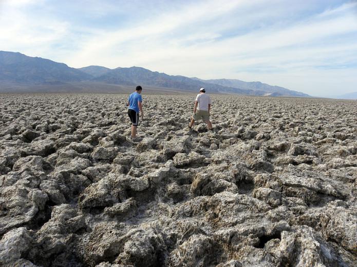
Certain types of sedimentary rocks are, by their very nature, indicative of certain climatic conditions. For example, in the arid subtropical regions, evaporation rates are so high that waters near the margins of the oceans readily evaporate. Once salinities reach certain levels, a sequence of minerals begins to precipitate directly from seawater. These minerals include gypsum (CaSO4H2O), anhydrite (CaSO4), dolomite (CaMg(CO3)2), halite (NaCl), and sylvite (KCl). The group of minerals is known as evaporites, and when found in the geologic record, are indicative of arid climates. Today the suite of evaporite minerals is being formed in the Persian Gulf. In the past, very thick sequences of evaporites were deposited in the Mediterranean during the late Miocene (6 million years ago), and in Texas and New Mexico during the Permian (250-300 million years ago).
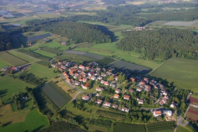
Just as evaporates indicate hot and dry climates, occurrences of coal in the geologic record suggest hot and wet climates. Today in tropical and subtropical regions with ample rainfall, trees, and other plants grow quickly. For example, tropical rainforest cover large areas in the Amazon basin, and mangrove forests grow along subtropical coasts in places like the Mississippi Delta and the coast of Florida. When this vegetation dies, it is rapidly buried in sediment in rivers, deltas, and beaches. Once encased beneath hundreds of meters of overlying sediment, and heated and pressurized over millions of years, the vegetation is transformed into coal. So just as evaporites are indicative of hot and dry conditions, coal is a sign of hot and wet conditions in the geological record. Please take a few moments to check out the photographic evidence below.
Coals and Evaporites Examples
Ancient Climate Events
In the next stage of the module, we will consider a number of climate events that took place in the geological record. The events we chose to present have one thing in common; they begin very abruptly, thus they provide some lessons about modern climate change. The events include both warming and cooling intervals and span a large part of the geologic record from over 2 billion years ago to 8.2 thousand years ago.
Ancient Climate Events: Pleistocene Glaciation
Ancient Climate Events: Pleistocene Glaciation
Some of the most abrupt and dramatic climate changes occurred very recently in Earth’s past, a geologic heartbeat ago if we consider the complete 4.6 billion years of the planet’s history. Materials including sediments deposited in the deep sea, ice formed in massive glaciers, stalactites formed in caves, wooly mammoths, and other large mammals, and spores and pollen of plants, provide evidence for very large and frequent oscillations in Earth’s climate that began about 2.5 million years ago. These oscillations involve the repeated advance and retreat of glaciers in the Northern Hemisphere. At their peak, ice-covered the northern parts of North America, Europe, and Asia, and the climate fluctuations also caused major changes in vegetation and animal habitats, as well as significant changes in ocean circulation.
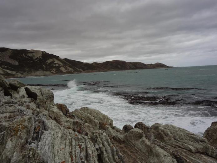
Glaciers deposit very diagnostic landforms and sediments that are often full of large boulders eroded from wide swaths of land over which the ice has traveled. More than a century ago, geologists determined using such evidence that at the coldest time of the Pleistocene, glaciers covered Edinburgh, Scotland; Moscow, Russia; and Detroit and Chicago in the US. In fact, from the glacial deposits alone, glaciologists had inferred several major advances and retreats of the two major ice sheets, the Laurentide in North America and the Fennoscandian in Europe and Asia.
At the height of the last major glaciation, known as the Last Glacial Maximum (LGM),18,000 years before the present, ice sheets covered Chicago, Boston, Detroit, and Cleveland (see maps below).
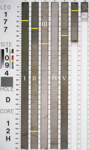
Our understanding of the climate of the Pleistocene surged in the 1950s when coring of sediment began in the deep sea and when the potential of oxygen isotopes in reconstructing ancient climate began to be realized. Cores showed dramatic alternations or cycles in the type of sediment with sharp color changes from red or pink to white or gray. The cycles were found to correspond to changes in the amount of the mineral CaCO3 that is derived from the shells of deep-sea organisms. The alternations were interpreted as major switches in the circulation of the deep ocean with corresponding changes in the ventilation and corrosiveness of the waters in which the sediments were deposited. Planktonic foraminifera, in different phases of the cycles, were found to have different oxygen isotope ratios that were interpreted as fluctuating sea surface temperature and glacial ice volume.
From studying cores of ice and deep-sea sediment, we now know that there have been more than 25 different advances and retreats over the last 2.5 million years. In fact, as the sediment and ice cores were gleaned, it was found that a number of the proxies fluctuated in a regular and periodic fashion. It had long been known from theoretical astronomy that the Earth’s orbit around the sun varies as a function of regular fluctuations in the shape of the orbit (called Eccentricity), the tilt of the axis of rotation (called Tilt or Obliquity), and the wobble of that axis (called Precession) (please see video below). Since these fluctuations control the amount of solar insolation received at the Earth’s surface, there was known to be a strong climate effect. These changes are cyclic with regular frequencies (the time from beginning to end of one cycle). From astronomical theory, the Eccentricity cycle is known to have a frequency of 100,000 and 400,000 years (two different cycles), Tilt/Obliquity a frequency of 40,000 years and Precession a frequency of 20,000 years. The Pleistocene proxy records were found to contain some of the same frequencies as these orbital fluctuations, and this is proof that changes in the amount of solar insolation were the ultimate control on the Pleistocene ice ages. The figure below shows an oxygen isotope record with prominent 41,000 and 1000,000-year cycles.
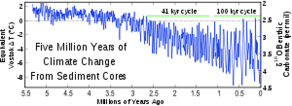
Credit: Five Myr Climate Change [24] from Wikimedia, licensed under CC BY-NC-ND 2.0 [25]
The video below provides an overview of how the Earth's orbit varies and how it affects climate.
Video: Earth's Orbit and Climate (1:49)
The Earth's orbit around the Sun varies in a number of ways that impact the amount of solar radiation and its distribution on the Earth's surface. This variation is cyclical, meaning that over a number of years the parameter increases and decreases in a periodic fashion. The orbital parameters can be observed in a number of paleo-climate records ranging from the waxing and waning of ice sheets to paleo-temperature records. The first orbital parameter is known as eccentricity. This has a cycle of 400,000 years and 100,000 years and describes the shape of the Earth's orbit around the Sun, which varies from a shape that's more elliptical to less elliptical. The second orbital parameter is known as obliquity. It's also known as tilt, and this parameter has a periodicity of 41,000 years and it describes the tilt of the Earth's axis as it circles the Sun. The third parameter is known as precession. Precession has a periodicity of 23 thousand years and precession describes the time of year at which the earth is closest to the Sun and farthest away from the Sun. All three parameters describe the amount and distribution of solar radiation received at any point on the Earth's surface.
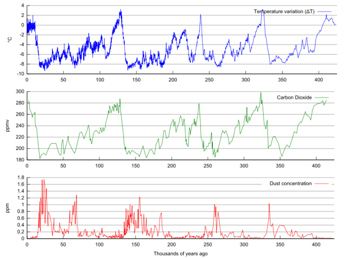
The figure below shows temperature (derived from O-isotopes), atmospheric CO2 measured from gas bubbles, and dust concentrations in ice samples from the famous Vostok ice core from Antarctica. The climate fluctuations shown by these data are some of the most abrupt and regular in the geologic record. The data show a close relationship between temperature and atmospheric CO2 content that is not fully understood but probably is related to intensified ocean circulation during glacial intervals that led to vigorous upwelling in the Southern Ocean. The Southern Ocean is one of the most productive areas in the oceans and intensified upwelling and photosynthesis could have led to the increased removal of CO2 from the atmosphere. Intensified atmospheric circulation during the glacial periods is thought to have transported more dust over Antarctica causing the increase in dust concentrations.
As the study of the Pleistocene period has intensified, we now know that glacial-interglacial cycles also corresponded to:
- more pronounced temperature changes in the high latitudes than the low latitudes (regions near the tropics). Temperature changes in high latitude regions are thought to be about 10oC between glacials and interglacials. The variation in oxygen isotope ratios of tropical planktonic foraminifera are thought to be largely a result of ice volume changes, not temperature changes;
- abrupt swings in atmospheric circulation with wind belts such as the Intertropical Convergence Zone (ITCZ) shifting latitudinally by several degrees;
- rises and falls of sea level by up to 120 meters and advances and retreat of the shoreline across the continental shelves;
- massive floods of freshwater down rivers such as the St. Lawrence and Mississippi rivers at times when the ice melted;
- northward and southward movements of vegetation belts across the continent.
You will notice one key thing from the temperature plot above. The temperatures were higher than today about 125,000 years ago -- this interval is known as isotope Stage 5e or more informally the last interglacial. Since this time was well before humans were producing large volumes of CO2 the warming was a result of natural processes related to Earth’s orbital configuration and insolation. So this is a key interval and one very interesting facet of it is that sea levels were higher than they are today likely by between 2 and 5 meters. Since temperatures were about 2 degrees C higher during the last interglacial, this gives us some important constraints on how fast sea level may rise in coming decades depending on CO2 emissions.
The last glacial peak occurred 18,000 years ago, and since that time the planet has been steadily warming (with a number of reversals as we will see shortly). Since these fluctuations in the Earth’s orbit continue, at some stage in the future, Earth will begin to cool. At the last glacial, maximum temperatures were considerably cooler in the high latitudes. Also, the sea level was over 120 meters lower.
Video: Feedback (:57)
Feedback is when a natural process amplifies or dampens climate change. The feedback may be positive when the natural process amplifies climate change, or negative when the natural process dampens climate change. An example of positive feedback is methane dissociation in permafrost. Warming leads to the breakdown of permafrost, leading to the outgassing of methane into the atmosphere, which leads to more warming, which will, in turn, lead to more methane dissociation in permafrost. An example of negative feedback is the weathering cycle. Global warming amplifies weathering and weathering draws down C02, which will dampen further global warming.
These fluctuations have significant potential in informing us about future climate changes. For example, the shape of the glacial climate cycles illustrates that the warming arm is rapid but the cooling arm is much slower. This distinction tells us about the mechanics of positive and negative feedbacks in Earth's climate.
Check Your Understanding
Pleistocene Question
Ancient Climate Events: Snowball Earth
Ancient Climate Events: Snowball Earth
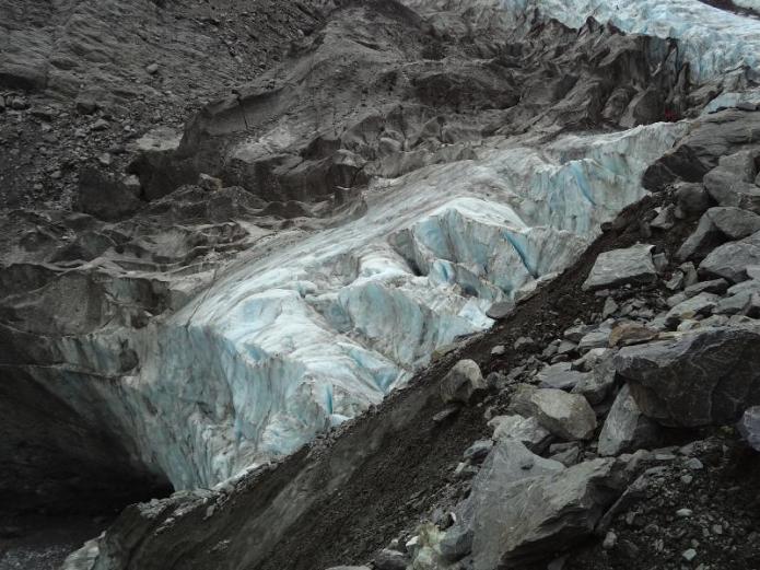
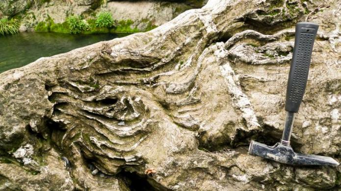
At the other end of the temperature spectrum from the PETM are the Snowball Earth events that occurred in the Proterozoic Era (543 million to 2.5 billion years ago), a time when only very primitive organisms inhabited the planet and oxygen levels were considerably lower than today. The aptly named Snowball Earth represents some of the most bizarre climate conditions ever experienced by the Earth, with strong evidence for ice sheets in equatorial locations. The evidence comes from sedimentary layers with a mixture of fine particles and large boulders, that look just like the rocks deposited by modern glaciers. These layers are found at locations known to be near the poles, which is not surprising, but also at those that are thought to have been near the equator, which is really unusual. This apparent global distribution of layers is why the events are termed "Snowball Earth". The main snowball events occurred about 2220 million years ago (2.22 billion), 710 million years ago and 640 million years ago.
Underneath and at the front of modern glaciers lie thick sediments that are characterized by a wide mixture of different grain sizes, from clay all the way up to large, angular boulders. Very similar, jumbled rocks are found in the Snowball events. It is not a surprise that such deposits exist at high latitude locations where large ice sheets have existed at a number of times in the past. What is so unusual is that glaciers are thought to have covered the tropics. Continents have been moving throughout geologic time, so it's natural to ask how we know the locations of Snowball deposits back in the Proterozoic. The best evidence for this is the orientation of magnetic grains in the sediments.
Video: Evidence for Tropical Ice Sheets (1:36)
The earth has a magnetic field that is driven by motions of fluid iron in the outer core. This magnetic field acts like a simple bar magnet with motion lines traveling through the center of the earth then wrapping around the earth, pointing back towards the North Magnetic Pole, as shown in this diagram. As we can see, if one is standing close to the equator, the field will be fairly flat. Whereas if one is standing close to the pole, the field will be much more vertical. This direction is called the inclination. The magnetic field of the earth is captured in sedimentary and igneous rocks, at the time of their deposition and formation. That means geologists can capture these rocks or sample these rocks, take them to the lab and measure the field when they were formed. If the field is flat, that means the rocks were formed closer to the equator and if that inclination is closer to vertical, that means that the rocks were formed close to the poles. For the snowball earth hypothesis, it is very very interesting that many of the rocks that capture glaciation, that contained evidence of glaciation, were formed close to the equator with flat inclinations, and this is one of the major pieces of evidence that glaciers covered equatorial regions during the snowball earth.
Credit: Tim Bralower © Penn State University is licensed under CC BY-NC-SA 4.0 [3]
So how cold was the Snowball Earth? If, as it appears, the planet was covered by ice from pole to pole, all of the sun’s radiation would be reflected back to space and temperatures must have been frigid. Models suggest that the global average temperature was about -50oC and the temperature at the equator would be similar to that at the poles today, about -20oC. With these conditions, most parts of the planet would have been under ~1 km of ice. With no ability to retain heat, it is hard to imagine how Earth recovered from a Snowball event, but surprisingly the end of the glacial events appear to have been extraordinarily abrupt.
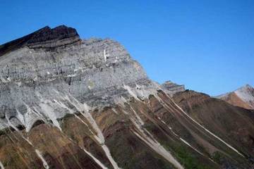
An integral part of the Snowball story is that the glacial layers are overlain by layers called cap carbonates, shown in the image to the right. These layers contain no glacial material at all, being composed entirely of the minerals calcite (CaCO3 and dolomite (CaMg(CO3). These carbonates look like they were deposited in relatively shallow water on platforms in a similar setting to the modern-day Bahamas. The carbonates often have large ripples formed by strong underwater currents, as well as evidence for bacterial activity.
The juxtaposition of glacial deposits and cap carbonates have fascinated geologists and spurred a lot of debate. Among the major questions that have been puzzled over are how glaciers could have melted so fast and how such concentrated carbonate material could have been deposited. The abrupt melting of ice must have been driven by the build-up of CO2in the atmosphere. Atmospheric CO2 is provided by processes such as volcanism, which presumably continued during the Snowball. CO2 is removed by processes such as photosynthesis and weathering of rocks, however, neither of these processes would have been active during a Snowball. Thus, it is thought that CO2would have risen unchecked to a point when a super greenhouse radiative effect was triggered, global temperatures rose rapidly, and the ice melted.
The origin of highly concentrated carbonate is likely connected to the ability of weather reactions to increase the saturation of minerals such as calcite and dolomite in the ocean. Perhaps more perplexing is how life, primitive as it was at the time, survived on a glacial planet. Available fossils suggest that organisms at the time included both cyanobacteria that used chemicals as a source of energy and also red algae that used light. Microbes are known to exist close to the surface of modern glaciers. Perhaps the ice was considerably thinner near the equator, or possibly there were small ice-free refuges. The Snowball remains a fascinating climatic puzzle.
Check Your Understanding
Ancient Climate Events: Paleocene Eocene Thermal Maximum
Ancient Climate Events: Paleocene Eocene Thermal Maximum
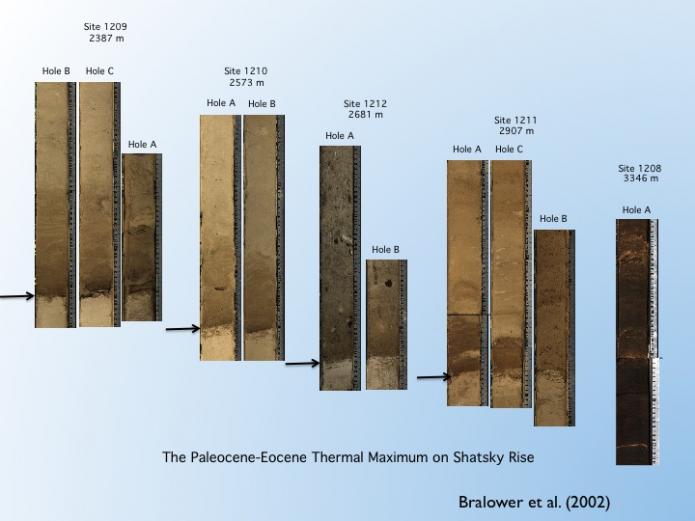
The Paleocene-Eocene Thermal Maximum (PETM) at 56 million years before present is arguably the best ancient analog of modern climate change. The PETM involved more than 5oC of warming in 15-20 thousand years (actually a little slower than rates of warming over the last 50 years), fueled by the input of more than 2000 gigatons (a gigaton is a billion tons!) of carbon into the atmosphere. The PETM was associated with the largest deep-sea mass extinction event in the last 93 million years and remarkable diversification of life in the surface ocean and on land. Because of its potential significance, geologists have swarmed to study the event, and it's been the topic of great interest, and more than a little controversy, for the last 25 years. For this reason, also, we devote considerable attention to the event here.
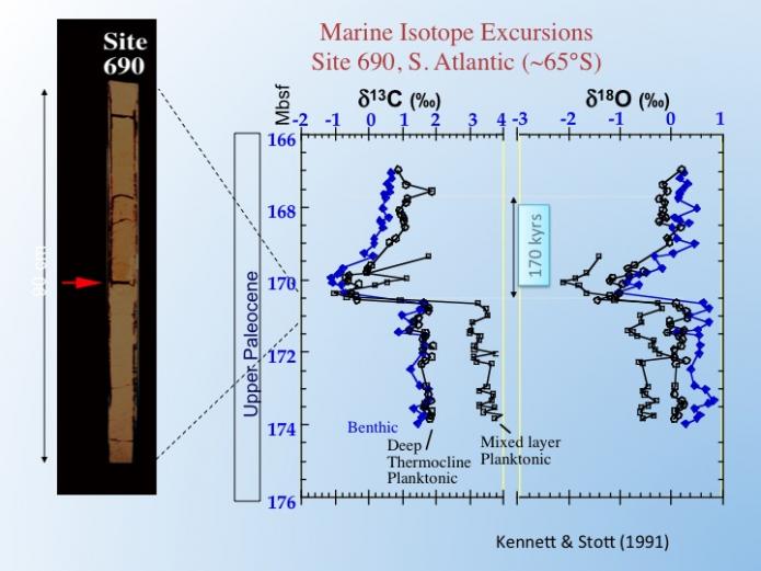
The evidence for warming comes from a variety of sources, the most compelling of which is the oxygen isotopes of planktonic and benthic forams in deep-sea cores. These data suggest significant warming of 6-8o C of ocean surface waters at a range of latitudes, as well as of deep waters. We don’t need to go into the detail here, but this converts to 4-5 oC of the average Earth temperature, which is pretty significant. For comparison, global warming since the industrial revolution is about 1.2 oC. Today, warming is a result of human activities, but only very primitive primates were around at the time of the PETM, and they did not drive cars (!), so what caused the warming back then?
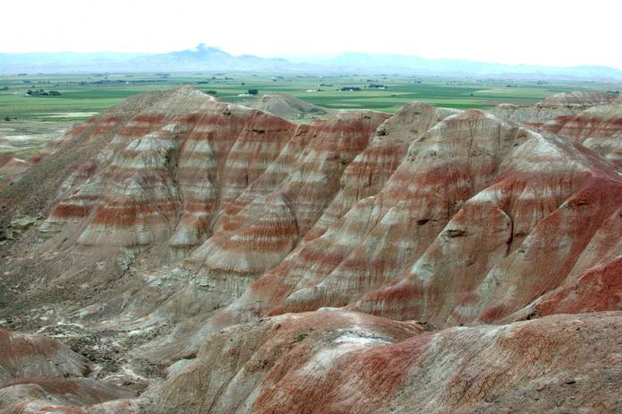
Corresponding to the oxygen isotope shift is a large and negative 4 to 5 per mil change in carbon isotopes that is used to define the geological extent of the event. The isotope excursion has been identified in sediments deposited in the ocean and those laid down in terrestrial environments such as lakes and rivers. It is called a golden spike because it can be correlated around the world and it marks a precise time horizon, in fact, the excursion is now the formal definition of the boundary between the Paleocene and Eocene eras. Moreover, the excursion in terrestrial sediments allows us to correlate the changes that occurred on land during the PETM with those that took place in the ocean. Below is what the PETM looks like in the Big Horn Basin in Wyoming.
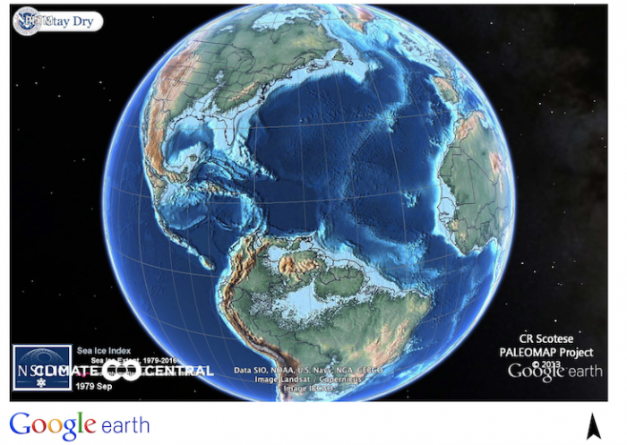
The content of CO2 in the atmosphere increased 3-4 times during the PETM. Regardless of whether it comes from cars, factories or from non-human sources, CO2 is a greenhouse gas, and it causes the atmosphere to warm. As a consequence, surface ocean temperatures at the peak of the event were extremely warm, especially in the high latitudes. Off the coast of Antarctica, a location today that is close to freezing, the oceans were about 20oC (68 oF) at the peak of the PETM! Imagine jumping into the ocean from Antarctica today! Tropical ocean temperatures were really hot. A recent paper indicates that temperatures off the coast of West Africa were 36 o C which is 97 oF! Now I’ve been swimming in Miami in August and it feels like a bathtub at 88 oF, but 97 oF is virtually uninhabitable! The PETM was also associated with major changes in the properties of the deep ocean. Unlike today, when deep ocean waters are characterized by temperatures close to freezing, PETM deep waters were 10-15o C. This may not seem that warm all considering, but there is no doubt that is caused a fundamental change in the way circulation in the ocean worked. Sea level was quite a bit higher during the PETM, and the continents were in different positions, as shown on the map below.
Likely, the cause of these warm deep waters was that they came from different surface ocean locations than they do today (see Module 6 for more detail on the sources of modern deep waters), combined with the warming that took place in the surface ocean. As warmer waters hold less oxygen than cold waters, PETM deep waters in many locations likely were possibly close to a condition that is known as hypoxia (we will learn more about this in Module 6). The word hypoxia does not sound too distressing but imagine for a minute that you are a fish, and you needed oxygen for respiration. Hypoxia would have been truly awful for such a creature! Finally, the input of so much CO2 into the ocean caused ocean waters to become more acidic and led to a condition known as ocean acidification (sorry to keep jumping ahead, but we will learn a lot more about this in Module 7!). Acidification of the deep ocean during the PETM is well accepted and is observed by complete dissolution of all CaCO3 shells that rained down on the seafloor. For creatures that require a shell for protection against predators and to protect the soft cellular parts from the harsh ocean, acidification would have been disastrous. By comparison, the shallow ocean experienced a much more minor decrease in its acidity and shelly creatures continued to thrive there.
PETM: Effects on Life
PETM: Effects on Life
Before you read this section, please make sure that you have read the section on different fossil groups under Proxy techniques: Fossils and Rocks
Paleontologists have studied the response of many different groups of organisms in the PETM fossil record, from tiny plankton such as foraminifera in the oceans all the way up to small primates on land. The event also has a spectacular plant record, especially if you love tropical species. One of the prime areas on land is in the spectacular Big Horn Basin in Wyoming where geologists have scoured the rocks for primates and plant material and an exceptional record of the PETM exists, correlated precisely to the deep sea record using the carbon isotope shift. The land record shows the introduction of small primates and tiny ancestors to horses right near the beginning of the PETM along with a burst of tropical vegetation (refer to photos). It's almost impossible for the primates and horses to evolve so quickly, what is much more likely is that warming during the event led to the opening of land bridges in places such as Alaska and Siberia and that appearance in North America is merely an immigration from another continent such as Eurasia. The beautiful Big Horn plant record shows a change from moist subtropical vegetation before the event to dry subtropical vegetation during it. Imagine the landscape in northern Florida changing in a geologic heartbeat to that of dusty southern Texas.
The task of studying fossils is the ocean in part of the PETM is somewhat difficult. PETM cores from the deep sea are devoid of CaCO3 in the early part of the PETM as a result of acidification of the deep ocean. This acidification was so strong that shells that had already been buried on the bottom of the ocean also dissolved! The chief biological impact of the PETM was the mass extinction of deep-sea benthic forams. Approximately 35-50% of all species of this group went extinct during the event. Almost certainly, acidification was the main culprit, but it couldn’t have helped that the sea floor was often hypoxic and, in some parts of the ocean, food supply was limited. Life on the bottom of the ocean during the PETM was not fun, that is for sure!

Interestingly, the benthic forams were almost unaffected by the environmental impacts at the Cretaceous-Tertiary (K-T) boundary, a time when the dinosaurs and many other groups went extinct. This paradox reflects the fact that the PETM had a far more severe impact on deep-water environments, whereas the K-T boundary has more impact on the surface ocean and land.
Evidence for ocean acidification at the sea surface at the very outset of the PETM is more elusive, partially because the fossil materials of coccolithophores and planktonic foraminifera that would hold the evidence were dissolved as they rained down through the acidic deep ocean or lay on the seafloor. However, later in the event, the fossil record is spectacular. Coccolithophores display signs of deformation, which has been observed in modern species grown in the lab under elevated CO2. So, it could be that there was a minor amount of acidification in the ocean surface. This is confirmed by a proxy for pH based on boron isotopes. But acidification was clearly not the driver of change among animals and plants that lived at the sea surface.
Although extinction was focused in the deep sea, the PETM actually did result in abrupt changes to life in the surface ocean, one of the most dramatic of which was the occurrence of blooms of dinoflagellates in the coastal oceans.
These dinoflagellate blooms, which can be thought of as ancient red tides, are a sign of major environmental stress in the coastal zone possibly as a result of the increased runoff of water from the land. This runoff delivered nutrients from the land which resulted in a process called eutrophication which led to rapid blooms of algal growth and hypoxia on the sea floor. Elsewhere in the oceans, the environmental changes during the PETM led to shifts in the distribution of plankton groups, with tropical species invading the high latitudes and high-latitude species dwindling in abundance. As we said earlier, the tropics could have been like a warm bathtub (close to 100o F) so you can imagine all of these tiny coccolithophores and foraminifera fleeing these conditions in a mass exodus! Clearly, temperature was the big factor for surface plankton away from the coastal zone.
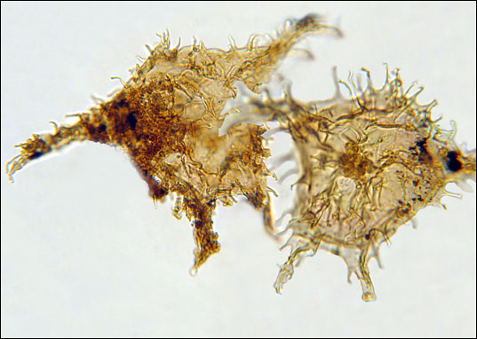
Another very cool aspect of the change in plankton is shown by the tropical and subtropical planktonic foraminifera, which contain a unique set of morphologies during the PETM. It’s unclear whether these morphologies represent new species or just variations of existing species, but it's pretty amazing that such variation arose in a geologic heartbeat and then disappeared at the end of the event. Quite possibly, these new forms represent the adaptation to a deeper environment, the species were forced to exodus the very surface of the ocean because of the uninhabitable conditions.
One final thing about the plankton during the PETM. At the end of the event, the distributions and abundance of different taxa reverted to close to where they were before. The structure of communities changed a little, but for the surface species, it was almost as if the event never happened. Life there was very resilient, but on the sea floor, it was a different story, life was altered forever.

The chief biological impact of the PETM was the mass extinction of deep-sea benthic forams. Approximately 35-50% of all species of this group went extinct during the event. Although extinction was focused in the deep sea, the PETM actually did result in abrupt changes to life in the surface ocean, one of the most dramatic of which was the occurrence of blooms of dinoflagellates in the coastal oceans.
These dinoflagellate blooms, which can be thought of as ancient red tides, are a sign of major environmental stress in the coastal zone, possibly as a result of the increased runoff of water from the land. Elsewhere in the oceans, the environmental changes during the PETM led to shifts in the distribution of plankton groups, with tropical species invading the high latitudes and high-latitude species dwindling in abundance. However, at the end of the event, the distributions and abundance of different taxa reverted to close to where they were before the PETM.
The burst of CO2 proposed for the PETM is consistent with the carbon isotope excursion as well as the rapid warming. Because the PETM involved very rapid warming and was caused by a burst of greenhouse gas, the event has been used to model the potential effects of modern climate change on life and the environment.
Faunas from the PETM
PETM: Causes
PETM: Causes
The source of the greenhouse gas is still the subject of active debate. One thing we know for sure, the PETM CO2 could not have come from humans or those early primates! There are five potential candidate causes: (1) gas hydrates in marine sedimentary rocks, (2) coals in terrestrial sedimentary rocks, (3) extensive wildfires, (4) melting of permafrost, and (5) volcanism in the North Atlantic Ocean coincident with the opening of the sea between Norway and Greenland. Each of these sources could have liberated sufficient CO2 or methane (CH4) to cause the warming and the carbon isotope excursion. This is explained in the video below.
- Gas hydrates are ice-like structures that hold methane (CH4) that, like CO2, is a powerful greenhouse gas. These compounds are only stable at a combination of pressures and temperatures not found at the surface. Today, these conditions exist several hundred meters below the seafloor along continental margins like off the coast of Florida, but in the past, they may have been stable at shallower burial depths.
- Coal is found interlayered in rocks under the surface in Norway and Greenland, and it has been hypothesized that volcanic lava injections in the subsurface could have driven methane from the coal and released it to the atmosphere.
- There is some evidence for wildfire during the PETM. Sediments deposited during the event in New Jersey and Maryland contain charcoal. However, so do sediments above and below the event, so this is not unique.
- Permafrost is like frozen soil that is often rich in plant material, contains a lot of methane and is a possible source of warming today. The concern is that warming due to human CO2 emission will melt permafrost, allowing it to release its methane into the atmosphere. Since the Earth was already warm before the PETM, there was probably not a lot of permafrost, so this mechanism is somewhat unlikely.
- Finally, volcanism occurred in the North Atlantic as the ocean opened up between Norway and Greenland. This volcanism included the injection of horizontal and vertical layers of magma (magma is lava below the Earth’s surface) as well as the release of volcanic CO2 into the oceans and ultimately the atmosphere.
Geologists have several ways to decide between these different mechanisms. There are independent means of determining the sources of carbon. The best way is the carbon isotope ratio of the different sources, which is very different. For example, methane hydrate has a ratio of – 60; coal and permafrost are about -20, while volcanism has a ratio of about -6. This means to cause an isotope excursion of -4 to -5, there needs to be almost 10 times more volcanic carbon than methane hydrate carbon.
Another way is the volume of carbonate dissolved by acidification in the deep sea. This can be estimated by looking at changes in the amount of CaCO3 in different sites. The third is from the magnitude of the change in pH, determined from the boron isotope proxy. Since the results from one proxy are not unique, geologists must use two proxies to constrain the source of CO2. These estimates give quite different results, unfortunately. Estimates from carbon isotopes and carbonate point to a source such as permafrost or coal, or a mix of volcanism and methane while those from boron and carbon isotopes and also point to a mixture from volcanism and one of the other sources. Thus, it is likely that there was a mixture of sources of greenhouse gas that fueled the PETM.
One of the key aspects of this debate is the evidence for some of these mechanisms actually exist. We know that there was volcanic activity in the North Atlantic, and dates from these lavas are almost precisely the same as the PETM. We know that this volcanic magma was injected through coal. There are also signs of disturbance on the sea floor off the coast of Florida that could have been caused by the release of methane hydrates. The evidence is thus stronger for volcanism, coal, and methane hydrate than it is for permafrost and wildfire, but the problem is far from solved.
One other key piece of evidence is the rate of CO2 addition. Methane hydrate, coal, and permafrost tend to be released in a more catastrophic fashion, whereas volcanism tends to be a little slower over time. If CO2 is released quickly, then a large part of it is absorbed in the surface ocean, leading to surface ocean acidification. On the other hand, CO2 added slowly generally bypasses the surface ocean and acidifies the deep. The lack of evidence for significant surface ocean acidification is more consistent with slow emission and volcanism.
One of the most important parts of the PETM is that it allows us to learn how the Earth operates in a warm mode with higher CO2 levels than today. As we learned, the current CO2 concentration in the atmosphere is 400 parts per million (ppm) and the PETM levels were likely double or triple this concentration (800-1200 ppm). Warm conditions during the height of the PETM led to increased break down of minerals, a process called weathering, and this removed CO2 from the atmosphere. It could be that increased weathering in the warm PETM atmosphere was the beginning of the end of the event. In addition, the process whereby the ocean absorbed CO2 leading to dissolution of CaCO3 would also have led to the termination of the event.
Video: Paleocene Eocene Thermal Max (2:00)
Understanding the ultimate cause of the Paleocene Eocene Thermal Maximum represents an unresolved problem. The mechanism must explain the large input of greenhouse gas that contributed to the warming, as well as a significant negative carbon isotope excursion. Currently, there are four candidates. The first is the dissociation of gas hydrates or clathrates, from underneath the ocean floor. Clathrates are molecules of ice and methane that are trapped at high pressure underneath the sea floor. If somehow, these molecules are exposed to atmospheric pressures, they rapidly dissociate and potentially deliver large quantities of methane to the atmosphere. The second mechanism is the inclusion of coals via dikes and sills upon the rifting of the North Atlantic igneous province. These coals and intrusions are found next to one another in places such as Greenland and Norway. Intrusion of the coal via hot material could deliver a lot of methane to the atmosphere. The third mechanism is the destruction of large amount of plant material via wildfires. This also has the potential to deliver large amounts of carbon dioxide to the atmosphere. Finally, the fourth mechanism, is the melting of permafrost. Permafrost will deliver large amounts of methane to the atmosphere once it is melted, and this also can explain both the carbon isotope excursion as well as the warming during the Paleocene Eocene Thermal Maximum. Ultimately, we will need more evidence to determine which mechanism can explain the event.
Check Your Understanding
Lab 1: PETM
Lab 1: Global warming during the Paleocene-Eocene Thermal Maximum (PETM)
Download this lab worksheet as a Word document:Earth 103 Lab 1 Practice Word Document [30] (Please download required files below.)
In this lab, we explore the magnitude of the warming that took place during the PETM based on proxy data. We compare PETM temperatures with current temperatures. We will look at Mg/Ca, oxygen isotope, and TEX-86 proxy temperatures from a number of cores of marine PETM sediments drilled in the oceans and on land, as well as margin analysis of leaves from land sections, to determine the temperature change. If you have not read the relevant material on proxies and the PETM in this module, please go back and do this before you begin the lab.
Note: The data for this lab are provided in Google Earth files. The goals of this lab are:
- To compare the magnitude and rate of warming at the PETM with that of today;
- To get comfortable with Google Earth software, especially turning maps on and off.
If you have not worked through the Google Earth Tutorial in the Orientation [31], you must do so now.
Files to Download
- PETM Data [32]
- PETM Paleogeography [33]
- Modern SST [34]
Get used to manipulating these files in Google Earth. This short video shows you the basics of how you will need to do this for the lab (and it will be critical for future labs too):
Video: Lab 1 Basics (3:15)
Hi students. I'm going to give you a quick tutorial as to how to open these Google Earth files for the PETM lab. And then I'll show you how to turn them on and off in Google Earth and to move around a little bit. This is going to be critical for doing the lab in module one. Okay, so the first thing you need to do is go to the lab, and I'm going to show you how to download a file. You just click on that file, like this, and then it'll open it directly in Google Earth Pro. You can see that. So I go "OK" and now it's opening my site locations with the site information. I'm gonna move the location here a little bit so that we're centered in the middle there. And let's say I want to open the Tanzania file to get the data out of it. I'm gonna click on that placemark, like that, and then I can read the data right off there. Oxygen 30.5 degrees centigrade pre-event; oxygen 41.9 degrees centigrade PETM. So you can then just type those numbers right into your spreadsheet. When I moved to another location, I'm gonna rotate it around, let's pick 527 site. And I click on that again, pre-event Magnesium calcium, PETM magnesium calcium, just put those right into your spreadsheet. It's really easy. Okay, so notice that my PETM data files are over here in my places. Right there, actually in my temporary places for now. When I close Google Earth, it will ask me if I want to save them. So you can turn this on and off just by clicking, like this, bingo off they go. Bingo, back they come. Alright, and then here are the other files that I've actually preloaded. My paleogeography, my future climate, and my current sea surface temperatures, paleogeography current temperatures, future temperatures. So if I want to turn on my paleogeography, I just go to click, and on it comes. You can see the locations of the continents, there we're a little bit different. I want to turn it off, BAM, off it goes. I want to turn on my future temperature file, there it is. This is for one of the climate reconstructions for the future. It's a bit blurry, but you can still read the numbers. You can see 2.4, .8. These are temperature changes that you'll be able to compare with the PETM warming, which was part of the last part of this lab. And then current sea surface temperatures, BAM, here it goes. There are my current sea surface temperatures and you have the scale at the bottom. So once again, you just need to make sure, as you go through this lab, that you're comfortable turning on and off these different layers because you'll need some of them on and some of them off at individual times, as is explained to you the instructions. So that's a quick go over as how to do the main functions that you'll need for module one lab. And please let Robert and me know if you have any questions and I will talk to you guys later on. All right, now I need to turn this off, and have a good day everybody.
Instructions
Load the PETM Data.kmz [32] file into Google Earth. The map shows continental positions and the extent of the ocean during the PETM. The red markers show the site positions that you will use for this lab. If you click on them, you will get several pieces of information: (1) the proxy used to determine temperature; (2) the temperature just before the PETM (pre-event) and (3) the PETM temperature. I recommend you make a table similar to the example below, that shows all of the data, as well as your calculated temperature change.
| Site Positions | Proxy | Pre-event Temperature | PETM Temperature | Temperature Change |
|---|---|---|---|---|
Next, practice turning on the modern sea surface temperature (SST) map in the Modern SST.kmz [34] file to compate the PETM temperatures with those of today.
Note that since the continents have moved a long way in 55 million years since the PETM, there are places in the PETM ocean which now lie in the position of the modern continents and thus don’t have equivalent modern temperatures (you will see some PETM sites in the dark blue area of the modern continents). But if you turn on the PETM Paleogeography kmz file, you will see more accurate reconstructions of the margins of the continents and the locations of the sites relative to them.
After you have made the table from the data that you collected and feel comfortable comparing the data with temperatures read from the temperature kmz maps, please answer the practice questions below. Once you feel good about your answers, go to Lab 1 in Module 1. There will be two labs available to you, Lab 1 Submission (Practice) and Lab 1 Submission (Graded). You will have a chance to answer practice questions and get the correct answers before taking the Lab 1 Graded questions for credit. Please make sure you fully understand the practice questions before you start the graded questions for credit. You may want to review some of the content in Module 1 to help prepare. Keep in mind that you will only get one chance to complete the graded labs.
Practice Questions
- What is the temperature increase at Bass River during the PETM (give your answer in degrees centigrade)?
- What is the temperature increase at Siberian Sea Site during the PETM (give your answer in degrees centigrade)?
- Which oceanic site (i.e., only site with numbers located in the ocean basins) has the smallest temperature change?
Now turn on the Modern temperature map and answer the following questions: - Compared to modern temperatures, is the location of Site 277 warmer or colder during the PETM?
-
Which oceanic site (i.e., only sites with numbers located in the ocean basins) has the smallest temperature difference between PETM and modern?
Module Summary and Final Tasks
Module Summary and Final Tasks
End of Module Recap
In this module, you should have mastered the following concepts:
- Geological materials offer valuable archives of ancient climate.
- This record can be deciphered using proxies for climate including stable isotopes, fossils, and leaf margin analysis.
- Rapid change between cold and warm climate occurred during a number of intervals in the Earth's past including the Quaternary (0-2 million years ago), the Paleocene-Eocene thermal maximum (55 million years ago), and the Snowball Earth (0.64-2.2 billion years ago).
- These events have the potential to inform us about changes to come including the impact of climate change on environments including the ocean and on life, and the processes that terminate warming events.
Assignments
You should have read the contents of this module carefully, completed and submitted any labs, taken the Module Quiz and added your entry and reply in the Yellowdig discussion. If you have not done so already, please do so before moving on to the next module. Incomplete assignments will negatively impact your final grade.
Lab
- Lab 1: PETM