Lesson 4: Earth's Interior
Overview
Lesson 4 will take two weeks to complete. In this lesson, we'll investigate the structure of the interior of the Earth. The Neat-o Interdisciplinary Idea for this lesson is optics. We'll complete a lab investigation of the index of refraction of water in order to make some simple observations about how light travels through materials with different optical properties. We'll extend this knowledge to seismic waves and then observe seismic waves to infer some simple aspects of the material properties of the interior of the Earth.
What will we learn in Lesson 4?
By the end of Lesson 4, you should be able to:
- List different methods scientists use to infer the material properties of the Earth's interior.
- Measure the angle of incidence and angle of refraction of light passing through water.
- Calculate the index of refraction of water.
- Use the index of refraction to predict raypaths through layered media.
- Pick P wave arrival times on a seismogram.
- Construct a travel time curve for P waves.
What is due for Lesson 4?
The tables below provide an overview of the requirements for Lesson 4. For assignment details, refer to subsequent pages in this lesson.
Lesson 4 will take two weeks to complete. 17 - 30 Jun 2020.
| Requirement | Submitted for Grading? | Due Date |
|---|---|---|
| Reading assignment: "Mineral physics quest to the Earth's core" and "Driving the Earth machine? " | Yes - We will discuss these two papers in a discussion forum in Canvas | multiple participation spanning 17 - 23 Jun 2020 |
| Optics lab | Yes - submit your worksheet to the Canvas assignment called "Optics Lab." | 23 Jun 2020 |
| Requirement | Submitted for Grading? | Due Date |
|---|---|---|
| P wave path problem set | Yes - submit your worksheet to the Canvas assignment called "P wave path problem set" | 30 Jun 2020 |
| Teaching and Learning Discussion I | Yes - this activity will be part of your overall discussion grade. The discussion will take place in the "Teaching/Learning I" discussion forum in Canvas | multiple participation spanning 24 - 30 Jun 2020 |
Questions?
If you have any questions, please post them to our Questions? Discussion Forum (not e-mail). I will check that discussion forum daily to respond. While you are there, feel free to post your own responses if you, too, are able to help out a classmate.
What's Down There?
In this lesson, we'll explore the Earth's interior. We'll find out what materials Earth is made of and determine their properties by making some measurements using seismic waves.
Earth's interior has 3 chemically distinct layers

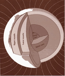
Let's start with a basic description of what's down there. Earth has three major concentric shells of chemically distinct material: the crust, the mantle, and the core. (See figure below and my screencast explanation.)
Click here for transcript
Here is a schematic diagram of a cross-section of the Earth. You can see this tiny thin part here is the crust. From the base of the crust, all the way to this boundary is the mantle. And from this boundary, all the way to the center of the Earth is called the core. We also distinguish between the upper and lower mantle. That is this boundary right here. And the inner and outer core. That is this boundary here. So how do we decide where to actually place these boundaries? That knowledge comes from observations of seismic waves. In fact, we can use observations of seismic waves to tell us a lot of other things about the composition of the interior of the Earth such as its exact mineralogic composition and the pressure and the density and temperature.
The crust is Earth's outer shell. It's the thinnest layer, but it is still important, mostly because it's where we all live! Also, during Earth's formation, when Earth became layered, the thin veneer of the crust retained some of the interesting metallic minerals that otherwise all went to the core because of their weight. This has been important for people because we've figured out how to extract these minerals and use them for industrial purposes. The crust is just a few kilometers thick at spreading ridges in the ocean, and as many as 50-80 km thick under continental mountain belts such as the Himalayas, but even at its thickest, the crust is quite thin compared to the radius of the Earth, which is about 6370 km. The most abundant rocks in the crust are silicate minerals, such as feldspar, quartz, mica, and amphibole.
The mantle occupies the most volume of the Earth; it extends from the base of the crust down to almost 3000 km depth. It is composed mostly of silicate rock, but denser forms of silicate than are commonly found in the crust, such as olivine, garnet, and eclogite.
The radius of the core is about 3000 km (almost half of the radius of the Earth). Its density is about twice that of the mantle. It is most likely made up of an alloy of iron and nickel, with some other heavy metals thrown in there as well.
The Earth has a dynamic interior
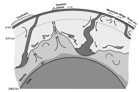
As models and measurements have become more sophisticated, the simple diagram above has been shown to be too simplistic. Instead, geophysicists envision a planetary interior that looks more like the figure below. (Also see my screencast explanation of the same figure.) Alternatively, you can read an approximate text transcript of my screencast of the modern view of Earth's mantle [2].
Click here for transcript
This schematic diagram is a much more up to date version of what we think is going on in the interior of the Earth, at least in the mantle. The take-home message here is motion. See all these little black arrows everywhere. They are showing you that the mantle is not actually just statically sitting there. It is moving around all the time. The thing that drives that motion is internal heat. The core has a lot of excess heat from the formation of the Earth and from the decay of radioactive elements. It needs to get rid of that heat somehow. The way it does it is by convection. That means moving hot material from one place to another where it can give that heat away. From the core mantle boundary up, first of all, you have got this weird D double prime layer where strange things happen to seismic waves that get in there. Here is a plume of material that is buoyantly rising because it is hot. This has been posited to be the source for hot spot volcanoes like this one in the picture here. We also have arrows that show things that are sinking. Right here is a cross-section of a subduction zone and you can see the slab is sinking. A lot of slabs get sort of hung up around 670 km depth. This is where the mantle has an increase in density and so it is harder for a sinking slab to get through there but they do get through most of the time. When they do the material that composes them piles up down here so it can later be recycled into whatever the rest of the mantle is doing. The take-home message here again is motion. But I want you to also remember that we are talking about solid rock here. It is by no means a liquid, so that motion is happening on very long timescales.
Notice all the little black arrows in the illustration above. Those arrows show movement of material in the mantle. The core loses heat to the overlying mantle. This heated material rises buoyantly to the surface. In this model, the core-mantle boundary is posited to be the source for mantle plumes that give rise to hot spot volcanism at the surface. You can also see some arrows showing heat escaping at a mid-ocean ridge. Heat escapes as new hot crust is formed at the ridges. Far away from a mid-ocean ridge, old cold oceanic lithosphere sinks at a subduction zone. Images from seismic velocity measurements show that these lithospheric slabs can sink all the way to the bottom of the mantle, where they pile up. Whether or not this material eventually becomes well-mixed with the rest of the lower mantle or remains in its own chemically distinct pool is still a topic of debate. So, the big idea to take home from this diagram is that the mantle of the Earth is in constant motion, driven by heat. This motion, however, is quite slow because the mantle is not a liquid, but is actually solid rock.
Quiz Yourself!

It is popular to demonstrate what goes on in the dynamic interior of the Earth by showing students a lava lamp. Can you identify the main similarities and differences between what goes on in a lava lamp and what goes on in Earth's mantle?
A lava lamp is similar to the mantle of the Earth because it has material that is heated, rises buoyantly, then cools and sinks. Convection.
A lava lamp is different from the mantle of the Earth because the Earth has an internal heat source, which is the heat of initial formation of the core as well as radioactive decay. In contrast, a lava lamp has an external heat source, usually a light bulb or something else that has to be plugged in or turned on. The mantle is solid rock and is composed of a variety of silicate minerals whose degree of mixing is still debated by scientists. It moves over long timescales. A lava lamp contains two immiscible fluids so that a person can have fun watching them move on short timescales.
But How Do We Know What's Down There? / Reading & Discussion Assignment
Observing the Interior
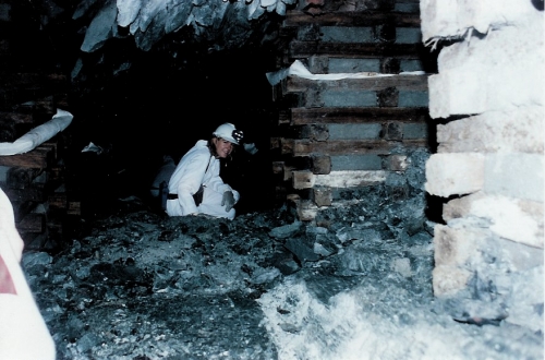
The deepest boreholes only go several kilometers into the Earth. A mine is the deepest place a person can go into the Earth (see Eliza, below) and while it's pretty incredible down there, even being deep in a gold mine does not offer much information about what the Earth is like hundreds or thousands of kilometers below the surface.
Seismic Waves
Since we can't go to the center of Earth, we have to rely on indirect observations of the materials of the interior. These observations mostly come from seismic waves. When an earthquake occurs, energy is radiated from the location of the earthquake in waves that travel through the Earth and arrive at seismometers at some distance from the source. The speed of these waves through the Earth is controlled by the properties of the material that the waves pass through. By measuring the time it takes for various waves to get from an earthquake to a given seismometer, scientists can back out what the material properties must have been like along the path taken by the wave.
Cool historical side note: The major boundaries of the Earth's interior were discovered by seismologists.
In 1909, Andrija Mohorovičić, a Croatian seismologist, discovered the boundary between the crust and the mantle by observing the sudden increase of seismic waves as they passed from the crust to the mantle. Because of the sudden jump in wave velocity, he was able to infer that there must be a change in the composition in the rocks at that depth. The boundary between the crust and the mantle is generally known as the "Moho" since most scientists had trouble finding the special characters needed to write Mohorovičić's entire last name correctly using a western keyboard. ha ha, only kidding. "Moho" is merely used because it is a shorter word. In 1912, Beno Gutenberg used observations of the sudden drop in P wave speed together with the observation of a "shadow zone" in which direct P and S waves do not arrive at seismograms a certain distance from the source (more on this later in this lesson) to calculate that the depth of the core-mantle boundary must be at about 2900 km. In 1936, Inge Lehmann observed a second "shadow zone" within the core itself to discover the boundary between the inner core and the outer core.
Laboratory Measurements
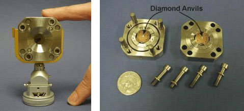
Seismic waves aren't the only way scientists try to figure out the properties of the interior of the Earth. Some geophysicists try to simulate conditions in the deep Earth by heating and squeezing likely mineral assemblages to see how they behave under the intense pressure and temperature regimes of the lower mantle and core. One way this is done is in a diamond anvil cell. The mineral assemblage of interest is squeezed between diamonds and sometimes simultaneously heated with a laser in an attempt to achieve the enormous temperature and pressure deep in the Earth. People are often impressed by the size of a diamond anvil apparatus, and I don't mean because it is so big! Check out the photos of one below.
Carbonaceous chondrites
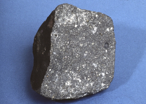
Geochemical theory also predicts the composition of the mantle and core. Meteorites give us information about the composition of the early solar system, and many of them have been dated to be older than the oldest crustal rocks on Earth. Carbonaceous chondrites, like the one in the photo below, are a special class of meteorites. Geologists think that these are representative of the composition of the whole Earth. So, by analyzing the elements contained in one of these meteorites, we should be able to back out the composition of our planet. This is one of the ways we've guessed at the composition of the core. Meteorites tell us that the Earth should have a lot more iron and nickel than what we have observed in the crust. It can't go in the mantle because the seismic wave speeds aren't fast enough and also we don't observe iron and nickel coming out of volcanoes that apparently have a deep mantle source. Therefore, the missing iron and nickel must be in the core.
Reading and Discussion Assignment
Read these two papers:
- Dubrovinsky, L. & J. F. Lin (2009). Mineral Physics Quest to the Earth's Core, Eos 90, pp. 21-22.
- Anderson, D. L. and S. D. King Driving the Earth machine? Science 346, 1184 (2014); DOI: 10.1126/science.1261831
The Dubrovinski & Lin article summarizes the state of the art among mineralogists who are studying the composition of the deep Earth. The Anderson & King paper offers a perspective that the asthenosphere is hotter than we thought and may be the source of non-subduction-zone volcanism. When you read them, think about the following questions for discussion:
Discuss in Canvas, starting with these questions
- What are the best guesses about the pressure and temperature at the center of the Earth? How did scientists arrive at these estimates?
- What does "seismic anisotropy" mean? What does the observation of seismic anisotropy in the inner core tell us about its structure?
- Look at the left panel of Figure 1 in the Dubrovinsky and Lin paper and compare it to the figure in the Anderson & King paper. How can you reconcile these two images?
- Explain the arguments against a deep mantle source for "plume volcanism" made by Anderson & King.
Grading criteria
You will be graded on the quality of your participation. See the grading rubric [4] for specifics on how this assignment will be graded.
Optics / Lab Activity
This lesson's Neat-o Interdisciplinary Idea is Optics.
Often, optics is a topic covered in a physics class, not necessarily in an Earth science class. However, having a good grasp about how light waves are refracted and reflected at the interface between two materials will help us later when we have to visualize how seismic waves travel through the Earth. That's why we're going to have a little optics lab experiment here. The ultimate overriding objective in this lesson is for you to make your own observations using real seismic data and be able to picture in your head how seismic waves travel through the Earth's mantle. Before we jump straight into an activity that uses seismic data, let's back up and make sure we understand some principles of optics.
Lab Activity
In this activity, we will calculate the index of refraction of water by measuring the angles of incidence and refraction of light as it passes from air to water.
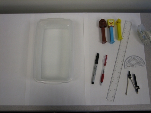
What you will need:
- Tank of water. A square or rectangular food storage container works well, as long as you can see through it and it is big enough. A fish tank would work really well, too. NOTE: You really do want to find a container that is big enough. If you can't or don't want to or it's not in your budget, it's okay, but just recognize that you are going to have a longer discussion of error and uncertainty at the end of the exercise. Why? Because if your container is too small, you won't be able to make observations over a wide range of angles of incidence.
- Paper
- Pen
- Straightedge
- Protractor
- Compass
- Three objects that you can see well when looking through the water. Upside down pushpins or screws work. I'm going to use Pez dispensers in my example.
The photo below shows my collection of materials for this activity.
Directions
-
Save the Optics Lab worksheet [5] to your computer. You will use this document to record your work in the remaining steps. The worksheet is in Microsoft Word format. You can use another format if you want to. You will submit your worksheet at the end of the activity, so it must be in a word processing, text, or image format I can open. Ask me if you think you have a weird format.
- Mark the location of the tank of water on the paper.
- Put one of your objects on one side of the tank of water so that if you look through the tank from the other side, you can see it through the water. I'm going to use Woodstock (see photo of step 3):
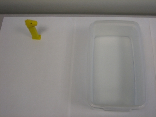 Illustration of step 3. Woodstock is standing on the left side of the tank of water.
 - Look from the other side of the tank at your first object and cover one eye (see photo of step 4):
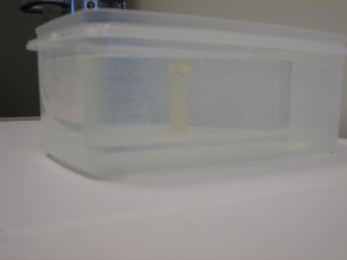 Illustration of step 4. I can see Woodstock through the tank full of water.
 - Now put one of your other two objects between your eye and the tank so that your first object is completely eclipsed (see photos).
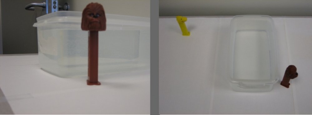 Illustration of step 5, eye view (left) and plan view (right). Chewbacca eclipses Woodstock.
 - Now put your third object between your eye and your second object so that the second object is completely eclipsed (see photos).
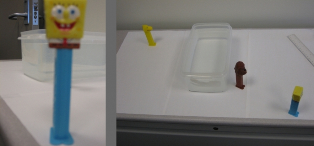 Illustration of step 6, eye view (left) and plan view (right). SpongeBob eclipses both Chewbacca and Woodstock.
 - Now take a pen and mark the location of your objects. I made a mark in the little divot right between their feet.
- Now you can take your objects and the tank of water away from the paper. You should have an outline of your tank and three dots drawn on your paper.
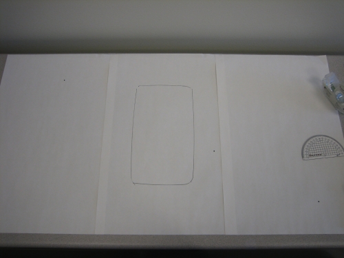 Illustration of step 8. There's the outline of the tank plus three dots showing the former locations of Woodstock, Chewbacca, and SpongeBob.
 - Connect the Chewbacca and SpongeBob dots with a line that extends to the outline of the tank.
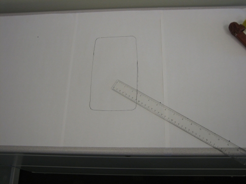 Illustration of step 9. Construct the incident ray with a straightedge.
 - Draw a line parallel to the Chewbacca-SpongeBob line that goes through the Woodstock point and connects to the outline of the tank on Woodstock's side of the tank. You can use a compass and straightedge to construct a parallel line. There is a Web site that gives a good tutorial showing how to do this: Math Open Reference [6]
- Use the straightedge to connect the two points on each side of the outline of the tank. Now you should have three line segments that show how light traveled from Woodstock through the air, through water, through air again, and to your eye.
Nitpicker Alert!
It is true that light was bent as it traveled from the air, through the wall of the tank and then through the water, then the wall on the other side of the tank, then the air again. Unless your tank has really thick walls, like, for example, the underwater viewing area of polar bear exhibits at zoos that have glass several inches thick, we should be able to ignore the effects of the thickness of the tank walls.
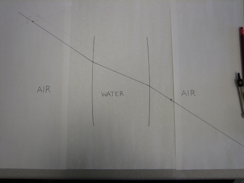 Illustration of step 11. There's the outline of the tank plus three line segments connecting the former locations of Woodstock, Chewbacca, and SpongeBob to the tank outline
 - Draw a line perpendicular to the tank outline at the point at which the incident ray from Woodstock to the tank intersects the tank outline.
- Measure the angle of incidence. This is the angle between the Woodstock-tank line segment and the perpendicular line.
- Measure the angle of refraction. This is the angle between the perpendicular line and the ray path inside the tank. See photo below.
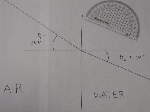 Illustration of steps 12, 13, and 14. The angle of incidence (θ1) = 33.5° and the angle of refraction (θ2) = 24°. Note that the protractor is just sitting there as a prop. I obviously did not measure the angles from way over there!
 - Replace the tank, put Woodstock in a different place and repeat the above procedure. You may also leave Woodstock in the same place and move your eye to a different place. Either way, repeat several times with either or both of the above variations.
- Using the worksheet for Lesson 4 Activity: Optics Lab, fill out Table 1 with your angle measurements.
- Eat all the Pez. This will ensure that your blood sugar is sufficiently high to carry out the next set of calculations.
- Continue completing the Lesson 4 Activity: Optics Lab worksheet.
Submitting your work
Submit your Lesson 4 Activity: Optics Lab worksheet. It should contain the plots you made and the answers to the questions at the end of this lab experiment. Please save your worksheet in the following format:
L4_Optics_AccessAccountID_LastName.doc (or whatever your file extension is).
For example, former Cardinals pitcher and hall of famer Bob Gibson would name his file "L4_Optics_rxg45_gibson.doc"
Then, upload your worksheet to the Optics Lab assignment in Canvas by the due date specified on the first page of this lesson.
Grading criteria
I will use my general grading rubric for problem sets [7] to grade this activity.
Snell's Law
Now that we are experts on how light is refracted as it passes from air to water, we can extend what we know to generalized waves passing through any medium. As long as we know the index of refraction, we should be able to describe the path a wave takes through some complicated layered structures. (See where we are going here? The Earth can be thought of as a big piece of material consisting of layers through which seismic waves pass.)
Snell's law describes the refraction of a wave passing through two materials that transmit the wave at different velocities:
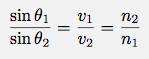
In words, the formula above says that if a wave passes from material 1 to material 2, the ratio of the sines of the angles of incidence and refraction (θ1 and θ2) will be a constant number and this constant number is equal to the ratio of the transmitting velocities of the two materials (v1 and v2) as well as the inverse ratio of the indices of refraction of the two materials (n1 and n2).
A diagram of what this formula means graphically is shown below.
.jpg)
Hopefully this rings a bell from the lab experiment we just did! In our experiment, our two materials were air and water just like in the diagram above. Air has an index of refraction of 1 (n1 = 1) and water has an index of refraction of 1.33 (n2 = 1.33).
Nitpicker Alert
Okay, actually a vacuum has an index of refraction of 1. Air at room temperature, pressure, and humidity has an index of refraction of about 1.0003. You'd have to design an experimental setup with a little more precision than what we did to resolve this discrepancy.
This means that we can use Snell's Law and calculate that the sine of the angle of incidence sin(θ1) divided by the sine of the angle of refraction sin(θ2) will always be equal to the ratio of the two indices of refraction, 1.33/1. This is what we confirmed in our experiment. Yay! Science works!
This also means we know that the ratio of the velocity of light through air to the velocity of light through water is equal to 1.33.
Quiz Yourself!
The velocity of light through air is 3 x 10⁸ m/s. What is the velocity of light through water?
Try it yourself and then click here to see my answer
The velocity of light through water is about 2.26 x 10^8 m/s. I got that answer by dividing 3 x 10^8 by 1.33.
Raypaths Through the Earth
The structure of the Earth makes tracing raypaths more complicated than the simple layered models we considered in the problem set. For one thing, the Earth is round, not flat. This means that all waves that start at the surface return to the surface, whether they encounter velocity changes along their path or not. Also, the concentric layers of material that make up the Earth aren't necessarily homogeneous. This means that sometimes waves are transmitted faster in certain directions than others. Let's discuss how raypaths travel through a homogeneous spherical body and then add complexity to see how seismic waves travel through a more "Earth-like" structure of concentric shells. Then we'll check out some actual seismic data to see how well the Earth mimics our simple model.
If the Earth were a Homogeneous Sphere
The animation below shows a cross-section through a homogeneous sphere. In this case, an earthquake that occurs somewhere on its surface would send seismic waves out in all directions and these waves would travel straight through to the other side.
This is a cross section through a homogeneous sphere. Let us just imagine that we have an earthquake that happened somewhere on the surface of the sphere over here. The wavefronts will travel outward from the source sort of like this, you know, the way that noise travels in all directions from a noise source. Or, if you toss a rock in a pond, the waves travel outward in concentric circles from the source. These are pictures of what the wavefronts look like. The ray paths are perpendicular to the wavefronts. We draw them like this. In a homogeneous sphere, all the ray paths would just travel straight through the sphere to the other side.
Hopefully you guessed that there was a point to all those refraction calculations you just did. What was that point? Well, the Earth is not a homogeneous sphere. It is composed of concentric shells of material and each one transmits seismic waves at a different velocity.
If the Earth had two layers over a homogeneous center
Let's consider a model like the sketch below, which is just a couple of spherical layers over a homogeneous center. This one is a little more Earth-like than the previous model we considered. When the incident ray strikes the boundary between the two layers, it will be refracted. It is refracted again at the next boundary, and then it happily travels along until it strikes the underside of that same boundary again and makes its way back up to the surface. In the animation below, note the shape of the ray paths through this model as opposed to the last model.
I've drawn here two layers over a homogeneous middle part. Each of these layers has a transmitting velocity. Let us say that each one of them is slower than the one below. Now let's say we've got an earthquake up here. One of the ray paths comes down like this. It hits this layer, and since the lower layer is a little faster, (you remember this, right) it is going to refract away from the normal, so it's going to go like that. Then it's going to do that same thing again because the third layer is even a little bit faster. Now it hits the underside of the layer and refracts back toward the normal and up. This can be generalized to any ray path that comes from this event. Here is another one. It even works if you have some ray paths that do not ever get as deep as that bottom layer. Here is an example of some ray paths that go through this layered media. Remember the difference between what this looks like and what the ray paths looked like in the earlier sketch where the Earth was completely homogeneous.
Earth model in which transmitting velocity increases smoothly with depth
Now what if you imagined a sphere composed of an infinite number of concentric layers, and let's say that each layer transmits seismic waves just a little faster than the layer above. This model in which velocity increases with depth is even more Earth-like than the previous model. At each local boundary, the ray still has to obey Snell's law, but since the layers are infinitely thin, the path ends up being a smooth curve. To see some of these curved ray paths, check out the animation below.
This model is even more Earth-like than the previous two. There are two big differences here. This model does not have a core in it, and also you need to have a little bit of imagination here because what I am hoping to have you think about is that you have got this gradation from dark to light that is smooth. I know you can see rings here but pretend they aren't there. what this model would show is if the Earth only had a mantle and it got successively denser and denser and denser from the outside to the inside, the waves would be transmitted faster and faster and faster. The effect of this would be to make the ray paths curved because at each layer's boundary the waves would still have to obey Snell's Law and refract, but if each layer is infinitely thin then mathematically that ends up being a curve. So let me just draw some sample rays. Here is an earthquake right here and so ray paths would curve like this or like that. Or like this. Anything that went straight down would just head through the middle but that is the only path that would be the same as the analogous path in a homogeneous Earth. Every other path curves. You might want to look back at the previous sketches to see the difference between these ray paths and the ray paths that went through a homogeneous Earth, or even the one that just had a couple of layers at the top.
Now, armed with our model of a sphere in which velocity increases with depth, we should be ready to plop seismometers down all over the world, measure the P and S wave arrival times from earthquakes, and confirm our idea about how wave speed varies in the Earth. In fact, seismologists did do this, and when they did, they realized that at some distances away from earthquakes, they didn't get any P or S arrivals at the times they should have arrived. They realized that there had to be a major boundary inside the Earth where material properties changed drastically, thus altering the wave paths enough to create a "shadow zone" where there are no direct arrivals from P and S waves. This is how the Earth's core was discovered. Seismologists knew that seismic rays took a curved path through the Earth. As the distance between the source and the receiver increased, the "turning point" (the deepest point along the wave's path) got a little deeper. At the farthest distance direct body waves were recorded, the turning point corresponding to that raypath must have been the depth of the mystery boundary, because a ray that tries to turn at a deeper point will run into that boundary, get refracted, and follow a different path. The depth of the boundary between the mantle and the outer core was found to be about 2900 km. This corresponds to a shadow zone for direct arrivals of P and S waves beginning at about 104° from the source. The same method was used to discover the inner core of the Earth as well.
A Seismic Record Section from the 2004 Sumatra-Andaman Earthquake
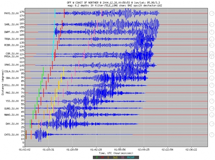
Let's check out some actual seismic data to see if we can distinguish all the features of the raypaths in the Earth-like models we considered. Below is a record section from the 2004 26 December Sumatra-Andaman earthquake. Creating a record section means plotting a suite of seismograms that are arranged in order by their distance from the earthquake. In this record section, the closest station is CHTO, at about 16 degrees away, and the farthest station is PAYG, at about 173 degrees away (Can't get too much farther than that because 180 degrees would be exactly on the other side of the Earth!). Each seismogram has some colored bars on it. These colored bars are arrival time picks for various body waves. Watch the two screencasts below the figure to see me sketch the paths the seismic waves took through the Earth to produce each of these arrivals.
Seismogram Arrivals Explained!

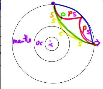
First I'll single out station SBA and draw a cross-sectional sketch of the Earth [8] that shows how each arriving wave gets from the earthquake to SBA.
This is a record section from the 2004 Sumatra Andaman earthquake. A record section just means that I have taken a bunch of seismograms and arranged them in order of their distance from the earthquake. So, on the x-axis here is time. On the y-axis is distance in degrees. Each of these seismograms is plotted with the name of its station and its distance away from the earthquake. What I'm going to do now is just focus on one of these stations. This station, SBA, here. I'm going to show you just by sketching that path that each of these arriving waves took to get from the earthquake to this station. These colored bars here are arrival time picks for various waves. This was probably done by an automatic picker that knows about how long it takes for each type of wave to get from one point to another on Earth. If I just make this little sketch right here of the Earth. I'm leaving out the crust here, but basically, this is a cross-section. Here's the mantle, and here's the outer core, and here's the inner core. And let us just pretend that my earthquake happened right up here at the top. We can pick any spot I guess. I'm going to choose this station SBA because it is handily almost exactly 90 degrees away and that is easy for me to freehand. So we'll draw a little house. That's our seismometer. The first arriving wave that gets from the earthquake to the seismometer is this one that is marked in green right here. It is the direct P wave. The path that the direct P wave takes through the mantle is kind of like that. Notice how it curves. It does not follow a straight line path. That is because seismic wave speed increases with depth. The next arriving wave is this arrival marked in red. That is PP. What PP does is it goes through the mantle and bounces once between the earthquake and the station, and then it continues on its way to the station. Each of these waves is a P wave in the mantle so we call it PP. The next arriving wave; well actually this orange one and this yellow one come practically on top of each other. The orange one is the direct S wave and the direct S wave follows the exact same path as the direct P wave only shear waves are slower so that is why it takes longer than the P wave to get from the earthquake to the station. The yellow one is a little more interesting. It is an S wave that bounces off the core mantle boundary and then gets to the station. So it is S and then that bounce point is called little c and then it is S again so the entire wave is called ScS. The next arriving wave is this pink one. The pink one is SS which follows the same path as PP only shear waves are slower so it takes it longer to get to the station. Those are all the waves marked here. We have this big high amplitude this coming in later on and those are actually surface waves. They travel along a path like this. Takes them longer to get there because the crust doesn't transmit waves as fast.
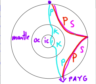
Now...Station PAYG is trickier! No direct P wave! No direct S wave! In fact, by looking at seismic records like this one, seismologists figured out that the Earth must have a core made of significantly different material than the mantle. Based on the "shadow zone," the distance range over which no direct mantle body waves are observed, seismologists also figured out the size of the core. The fact that no S waves could make it through the core showed scientists that at least part of it had to be a liquid. Watch my sketch of how this works for the arrivals at station PAYG. [9]
Let us look at the same record section, but a different station. This time I am going to look at station PAYG, which is almost 180 degrees away from the earthquake. I have drawn it down here. What you will notice right away is that the number of arrivals is fewer. There is no direct P wave and there is no direct S wave. The reason for that is that the core gets in the way. Remember at the earlier station that P waves and S waves take a kind of curving path through the mantle that I'm showing you right now with the mouse. If you are farther away than about 104 degrees then these waves will bounce off the core or they will be refracted within the core as P waves and so you will not get a direct arrival. This is how the core was discovered. What are the arrivals that are coming in at this station? The first one is this one here and that one is labeled PKiKP. What that wave does is, it is a P wave in the mantle, it comes down here, it gets refracted in the outer core, and the inner core, and back through the outer core, and back out through the mantle to this station. The path is called a P wave when it is in the mantle, and then a P wave in the outer core is called K. I do not know why that is. In the inner core it is called i. And then it goes back out as K and P. The whole thing together is called PKiKP. The next arriving wave is PP. That is our old friend. We know how that works. It goes through the mantle and it bounces and it goes to the station. Each of these paths is a P wave in the mantle. It is called PP. The last arriving wave is SS. It follows the same path as PP except shear waves are slower so it takes it longer to get there.
Want to make your own record section of a recent earthquake?
Thanks to the good folks at IRIS [10], the Incorporated Research Institutions for Seismology, it is not too hard for anyone to do. I recommend letting your students play around with this!

-
Go to Wilber3 [11], where you can request seismic data from recent earthquakes.
-
The default page has a map with recent (last month or so) earthquakes on it. The map is interactive, so you can draw a box to zoom in, and there are also some dialog boxes you can type into in order to narrow down the number of events in the list by date, location and magnitude.
-
The map locations are clickable colored circles. Clicking on one of them will highlight that event in the list on the same page.
-
After you've clicked on your selection in the list, the map will refresh and now show you all the stations that recorded data from your selected earthquake.
-
At this point you can click a button that says "Show Record Section"
What path does a P wave take through the mantle?
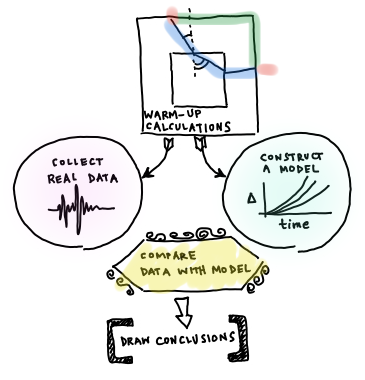
Motivation and Preamble
The Earth is optically opaque. Unlike the tank you used in the optics lab, you can't see through the Earth to verify what path a P wave takes on its way from an earthquake to a seismometer. How do we know what path a P wave takes? What data can we collect to help us find this out? We are going to take a two-step approach to answering these questions. We are going to collect some data from seismometers around the world that all recorded the same earthquake, and then we will use that data to plot a travel-time curve. We will then construct some models about what the data would look like given certain mantle properties. We will compare the data with our models to see if they match up or not.
What you will need:
You will need a plotting program, a scientific calculator, a protractor, and a straightedge to complete this problem set. Drawing software is only suggested if you have a program you are already adept at using, otherwise, sketch by hand.
Directions
You can save the P wave path worksheet [12] to your computer, and use it to record your work. The worksheet is in Microsoft Word format. To work on this assignment, you can use a word processing program, or even do it all on paper as long as I can read the scanned pages. You will submit your worksheet electronically, so it must be in a format I can open. Ask me if you aren't sure whether your format is weird. The downloadable worksheet has the same problems as are written out below; the worksheet is just to save you copy-and-pasting effort. This website has a couple of screencasted hints that are not in the worksheet, though.
Part 1: Snell's Law Warm-Up Calculations
Before we start jumping right into the data and models, we will do some warm-up calculations involving how rays travel. The point of this is so we have some intuitive sense later on about the meaning of our data and models, and what we might expect them to look like. In this part of the problem set, you will make calculations involving the refraction of waves through media and you will trace ray paths through media. You will have to make some sketches. If you want to use drawing software, go ahead. If you want to make your sketches by hand and take pictures of them, that is also fine. When I grade your sketches I will not be using a protractor to judge the precision of your angles, but I will be looking to see if your angles are correct relative to each other on the same sketch. For example, if the angle of refraction should be greater than the angle of incidence in a particular problem then you need to draw it that way.
The Problems
1.1 Calculate the angle of refraction for a ray of light passing from air to water with an incident angle of 45°. Assume the index of refraction of water (nwater) is 1.33 and nair is 1. Sketch the path of the ray through the water layer. 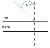
1.2 Calculate the angle of refraction for a ray of light passing from water to air with an incident angle of 30°. Assume the index of refraction of water (nwater) is 1.33 and nair is 1. Sketch the path of the ray through the air layer. 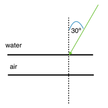
1.3 Suppose you have a ray of light that passes through three layers: air - water - air. The angle of incidence at the first air - water boundary is 20°. Calculate the angle of refraction at the first boundary in the diagram below and calculate both the angle of incidence and angle of refraction at the second (water - air) boundary. 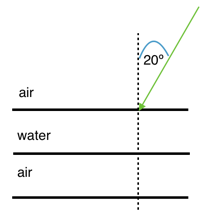
1.4 Now let's consider the path taken by a seismic wave instead of light. For the purposes of this calculation, we'll pretend the Earth is flat. An earthquake happens at the surface of a series of layers as pictured below. Consider a P wave that leaves the source along the path as shown in the cartoon and hits the boundary between the upper layer and the second layer with an angle of incidence of 30°. Given the transmitting velocities for a P wave in all the subsequent layers, sketch the path of the ray until it hits the bottom, and find all the angles of incidence and refraction along the way.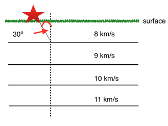
1.5 Let’s consider a seismic wave that passes through the square-shaped object below. In this object there is a fast center and an outer layer of slower material. The P wave leaves the source and hits the first boundary with an incident angle of 40°. Sketch the path taken by the P wave until it gets back to the outer surface of the square and calculate all the angles of incidence and refraction along the way.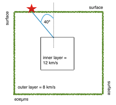
1.6 Now let’s say that same square-shaped object in #1.5 is actually homogeneous. Draw the path that the P wave would have followed to get from the source to the position of the “receiver” (where you calculated that it arrived at the outer surface in #1.5). Is the distance traveled as measured along the surface the same, shorter or longer as the distance as measured along the surface in #1.5? Is the actual path traversed by the P wave the same, shorter, or longer than the actual path traversed by the P wave in #1.5?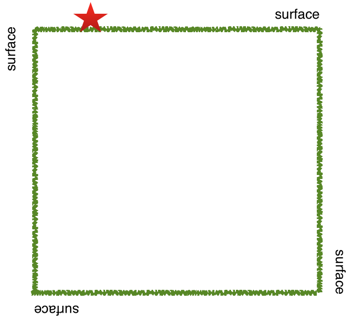
Road Check
Okay, so you just did a bunch of calculations and sketches. What's the upshot? Here's what we found out: Rays travel the fastest path they can. This will be a straight line path through a homogeneous solid, but might not be a straight line path in an object composed of different materials that transmit rays at different speeds. Rays change direction at the boundary between two materials.
Therefore, if the mantle is homogeneous then a P wave will take a straight line path with a constant velocity through it. If the mantle is not homogeneous then the P wave's velocity will not be constant all the way through and its path will not be a straight line. The obvious next step towards our goal of figuring out what path a P wave takes through the mantle is to collect some data about P wave velocities. We should look for data covering a variety of paths so we can compare if the velocities are all the same or not. What we want is to either go get data from a station that recorded P waves from earthquakes all over the world, or else get data from one earthquake that was recorded by stations all over the world.
We could do either one, but data is commonly archived by earthquake instead of by station, so it will be more convenient to collect data from a variety of stations that all recorded the same earthquake. Let's do it!
Part 2: Collecting data and making observations

In this part of the problem set, you will pick the arrival times of P waves on seismograms and use them to construct a travel time curve for P waves through the mantle. Then, you will compare this data to models of travel time curves for an assumed homogeneous mantle.
The seismograms for this activity are clickable thumbnails so you can work with a big version of each one. On this web page there are several hints about how to do most of the calculations.
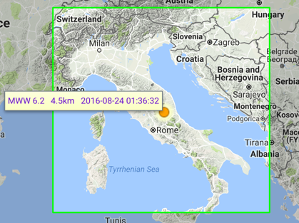
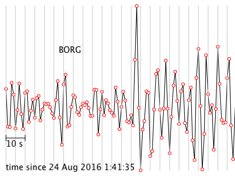
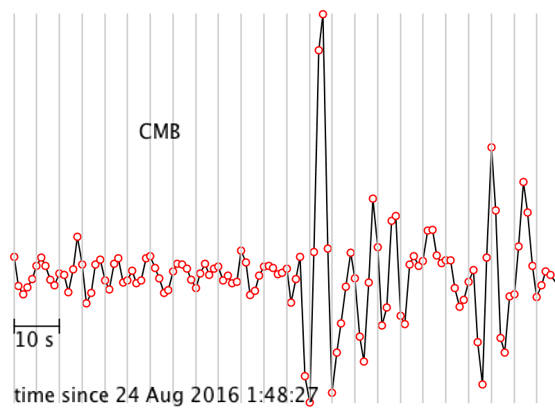
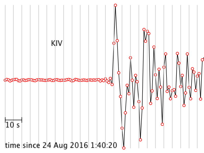
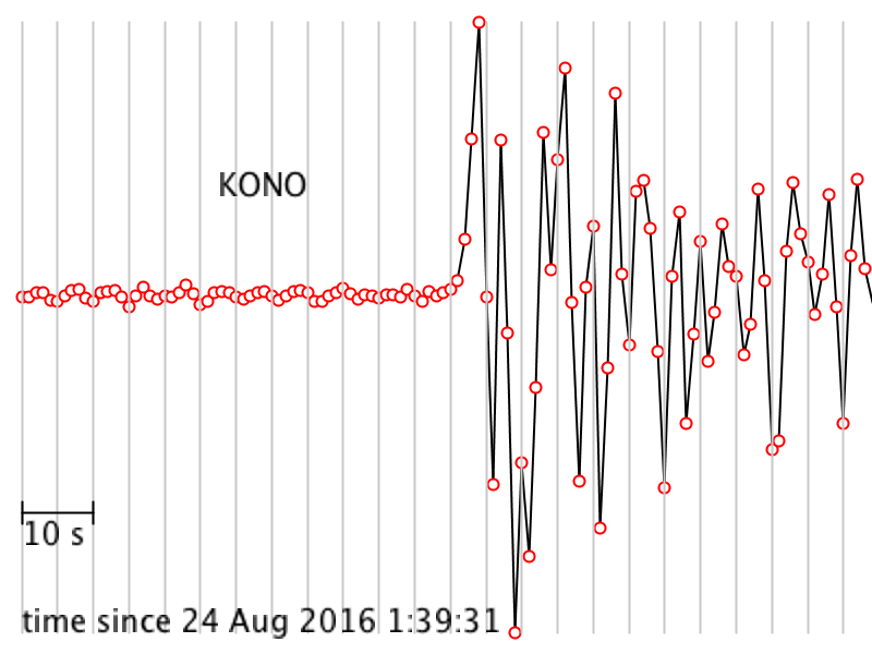
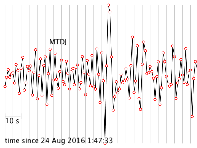
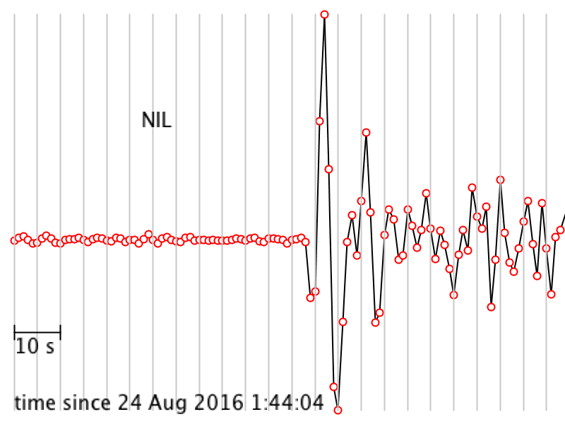
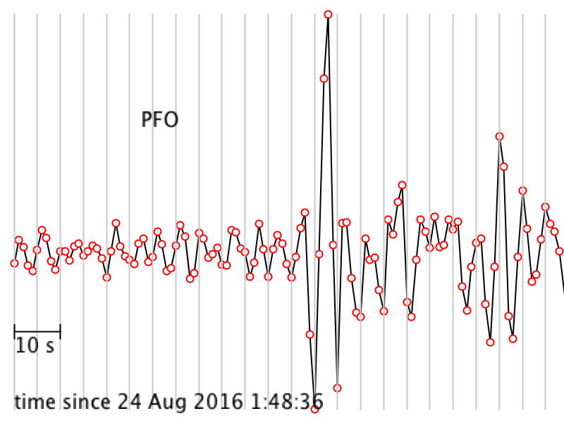
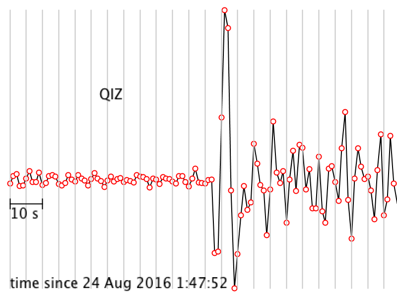
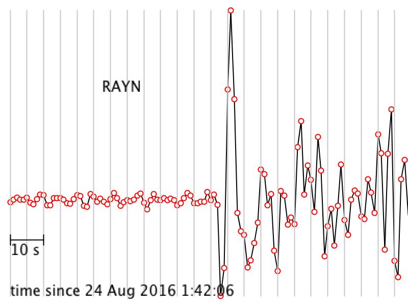
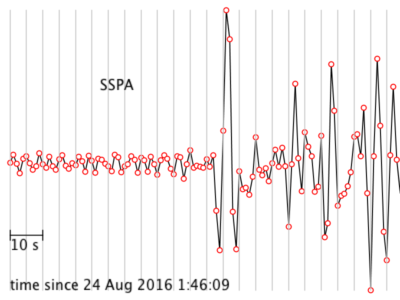
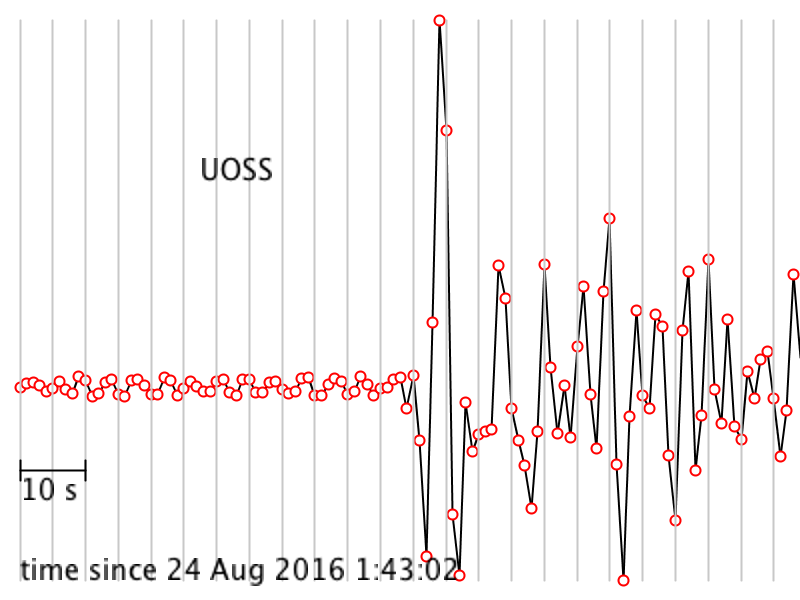
The seismograms you'll be working with are from the Amatrice, Italy, earthquake of 24 August 2016. Its location was 42.7226° N, 13.1871° E, and it happened at 01:36:32 UTC. All the seismogram times are also in UTC.
The Seismograms
 [13]
[13]
 [14]
[14]
 [15]
[15]
 [16]
[16]
 [17]
[17]
 [18]
[18]
 [19]
[19]
 [20]
[20]
 [21]
[21]
 [22]
[22]
 [23]
[23]
 [24]
[24]
 [25]
[25]
 [26]
[26]
The Problems
For #s 2.1, 2.2, and 2.3 I find it easiest to make a table in which I write down the station name in column 1, The P wave arrival time at that station in column 2, the travel time in column 3 and the distance in degrees in column 4. Doing so makes it easier to make plots and be organized. I am leaving it up to you to construct such a table, or if you hate tables, to ignore this advice.
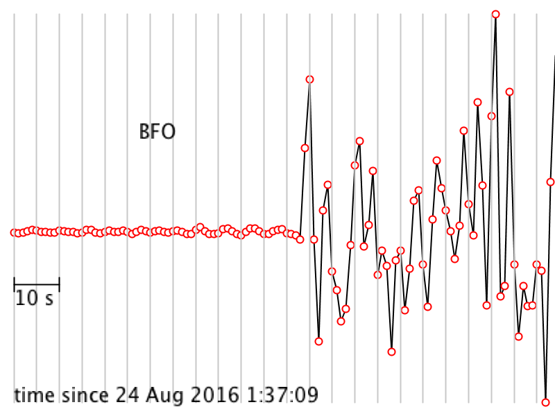
2.1 For each seismogram, pick the arrival time of the P wave. The P wave is the first impulsive arrival that rises appreciably higher than the background noise level. It can take a bit of skill and practice to pick arrivals on a seismogram, but at least P waves are easier than the later arrivals.
My tutorial for picking the arrival time of a P wave [27] (and a transcript [28])
2.2 Calculate the time it took the P wave to get to each station.
My tutorial for calculating P wave travel time [29] (and a transcript [30])
2.3 Calculate the distance between each station and the event in degrees. In order to do this, you'll have to compute the great circle distance between the event and each station. Here is the formula for great circle distance between two points on the surface of a sphere: cos(d) = sin(a)sin(b) + cos(a)cos(b)cos|c| in which d is the distance in degrees, a and b are the latitudes of the two points and c is the difference between the longitudes of the two points. Jean-Paul Rodrigue, at Hofstra University, provides an excellent explanation and tutorial of how to calculate distance along a great circle path [31].
My tutorial for calculating great circle distance [32] (and a transcript [33])
There is a nice website that will calculate the great circle distance for you [34] and it will give you the answer in kilometers, so if you use it, divide your distances by 111.32 to get from kilometers to degrees in order to make your plot in #2.4.
2.4 Make a plot of distance in degrees vs. P wave travel time. Note that choice of which quantity to put on which axis depends on what you are trying to do with this data. Many seismologists put distance on the x axis and travel time on the y axis because then the slope of the data is the quantity known as the “slowness.” However, doing it the other way around is also quite common, especially if you are stacking record sections to make a plot. You can choose.
2.5 Which station was closest and which station was farthest away? What were the distances between the earthquake and each of these two stations? What was the difference in arrival time between those two stations?
2.6. This event was large enough that it was recorded by stations even farther away than the farthest station you worked with. Why didn't I make you pick P waves for stations that were farther away?
2.7 We know the travel time of the P wave to each station and we know the surface distance between the earthquake and each station but we don’t know the actual path the P wave took and we don’t know whether velocity was constant along that path or not (Remember that those are the two things we are trying to find out in this lab exercise). So when we calculate velocity, keep in mind that it is an apparent, average velocity. What is the apparent average velocity of the P wave for the closest station? What is the apparent average velocity of the P wave for the farthest station? Are they the same or not? If they are not the same, can the difference be attributed to rounding during calculations, mistakes in arithmetic, or other uncertainties?
2.8 Look at your plot from #2.4 and describe how the apparent average velocity changes with station distance, if it does. For example, are the data randomly scattered with no relationship among them? Is there a smooth variation with distance? If there’s a smooth variation, does velocity increase or decrease? Or, does the velocity stay about the same? Are there sudden jumps?
Road Check
Up until now we have been collecting and analyzing a dataset chosen to help us figure out if the Earth’s mantle is homogeneous or not. The next step is to predict what travel time data would look like if the mantle is in fact homogeneous. Then we can compare it to our actual data and see what we find out.
Part 3: Construct a model and compare it to the data
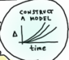 We will construct a model plot of travel time vs distance (like the plot in #2.4) except that we will set the velocity to a constant and we will calculate what the travel time curves should look like instead of using real data. Doing this is not quite as trivial as you might guess. It takes a little bit of trigonometry to do this correctly.
The Problems
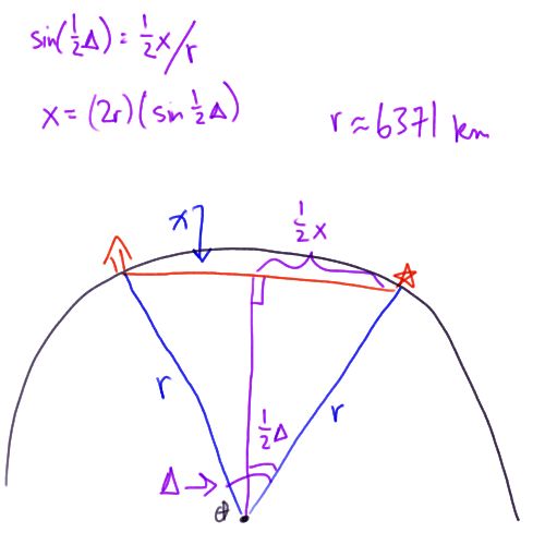
3.1 If the great circle distance between an earthquake and a station is 45º, what is the straight-line path distance through the Earth between them? (see hint cartoon and screencast below)
You can also read this transcript of me screencasting the right triangle sketch
Here is how to solve for the path length of a P wave through the mantle on the assumption that the mantle is homogeneous and transmits waves at the same speed regardless of depth.
I am just going to draw a hemisphere of the Earth. Here is the center of the Earth. Let us assume there is an earthquake that happens over here. And you have a seismometer over here that recorded a P wave. If the mantle is homogeneous it means that the P wave will travel a straight line path through the Earth from the earthquake to the seismometer. To solve this problem of what this distance x is, I am going to first draw a radius from the center of the Earth to my earthquake and another radius from the center of the Earth to the seismometer. This is an isosceles triangle because these two sides are both the radius of the Earth and then this other side here is the one we are trying to find. We also know something else about this triangle. We know this angle. This angle seismologists call delta, and it is exactly the great circle arc distance between the earthquake and the seismometer. You have already calculated delta for all the stations in this problem set. We drop a perpendicular line from x to the center of the Earth bisecting x and bisecting this angle delta. This is a right angle here, and this distance is one half x and this angle here is one half delta. The sine of one half delta is equal to the opposite side, which is one half x, divided by the hypotenuse, which is the radius of the Earth. Let us write that down. This is a fabulous expression because we know everything in it except x and we are trying to solve for x so that is awesome. Let us rearrange. x equals twice the radius times the sine of one half delta. If you want to find x you can just plug in delta, which you have already calculated, and the radius of the Earth, which we can take as 6371 km. That's a good approximation. And away you go. X is the distance between the earthquake and the station traversed by a P wave if you assume the mantle is homogeneous.
3.2 Suppose a P wave traveled along the path you calculated in #3.1 at a constant speed of 8 km/s. Calculate its travel time between the earthquake and the station.
3.3 Suppose a P wave traveled along the path you calculated in #3.1 at a constant speed of 10 km/s. Calculate its travel time between the earthquake and the station.
3.4 Suppose a P wave traveled along the path you calculated in #3.1 at a constant speed of 12 km/s. Calculate its travel time between the earthquake and the station.
3.5. Assume constant mantle velocities of 8, 10, and 12 km/sec. Draw the three travel-time curves that correspond to these velocities on one set of axes.
My tutorial for how to make your reference travel time curves [36] now that you know how to calculate the straight-line P wave path and find the travel time for a single station. (and a transcript [37])
 3.6. Combine your plot from #2.4 and your plot from #3.5 on the same axes. Can your data be fit with a curve representing constant velocity? Feel free to try other values for the velocity if 8, 10, and 12 don’t work.
 3.7. Time to answer the big question from the beginning of the problem set! Does the P wave follow a straight line path through the mantle? How do you know? Lead me through your logic and your observations from this lab to answer this question.
Submitting your work
Please save your worksheet and name it like this:
L4_Ppath_AccessAccountID_LastName.doc (or whatever your file extension is).
For example, former Cardinals manager and hall of famer Whitey Herzog would name his file "L4_Ppath_dnh24_herzog.doc"--This naming convention is important, as it will help me make sure I match each submission up with the right student! You can look it up; his given name is Dorrel Norman Elvert Herzog. Upload your finished product to the Canvas assignment by the due date listed on the first page of the lesson.
Grading Criteria
I will use my general grading rubric for problem sets [7] to grade this activity.
Teaching and Learning Discussion I
Let's take some time to reflect on what we've covered in the past two lessons!
For this activity, I want you to reflect on what we've covered in Lessons 3 and 4 and consider how you might adapt these materials to your own classroom or share the ways in which you already teach this material. Since this is a discussion activity, you will need to enter the discussion forum more than once to read and respond to others' postings. This discussion will take place over the second week of this lesson.
Graded Discussion Directions
- Enter the Teaching and Learning I Discussion Forum
- Post your thoughts.
- Read postings by other EARTH 520 students, too, and respond to at least one other posting by asking for clarification, asking a follow-up question, expanding on what has already been said, etc.
Grading criteria
You will be graded on the quality of your participation. See the grading rubric [4] for specifics on how this assignment will be graded.
Additional Resources and Bibliography
Additional resources
Web sites
Papers
- Irifune, T. and R. J. Hemley (2012). Synthetic Diamond Opens Windows Into the Deep Earth, Eos 93, 65-66.
Bibliography
Anderson, D. L. (1989). Theory of the Earth. Boston: Oxford. Blackwell Scientific Publications, p. 366
Dziewonski, A. M. & Anderson, D. L. (1981). Preliminary Reference Earth Model, Physics of the Earth and Planetary Interiors, 25 (4), pp. 297-356.
Summary and Final Tasks
By now you should have a handle on the material properties of the interior of the Earth. In this lesson you made some simple optical measurements and extended them to figure out some properties of the Earth's mantle. You know why seismic waves take the paths they take and about how long it takes them to do it. You also found out the current state-of-the-art thinking about how hot the center of the Earth is and what it is made of. Oh, and hopefully, you got to eat some Pez candy, too.
Reminder - Complete all of the lesson tasks!
You have finished Lesson 4. Double-check the list of requirements on the Lesson 4 Overview page to make sure you have completed all of the activities listed there before beginning the next lesson.