Elasticities and Demand Curve Shapes

Economics is a dynamic process. Given the millions of human interactions that make up an economy, it is not surprising that things do not stay the same for very long, if at all. Things change: this is the nature of a dynamic economy. We now ask, how much do they change?

At this point, this question relates to the shapes and slopes of the demand curves, which we will examine here. We will look at the supply curve in the next lesson.

In physics, the term “elasticity” refers to how much something stretches when force is applied to it. In economics, when we think about "elasticity,"we are interested in how much a quantity demanded or supplied will change when some “force” is applied to the market. Both the demand and supply curves have elasticities. Let us talk first about the elasticity of demand. The phrase “elasticity of demand” is incomplete: we are talking about the response of demand to something. So, for the title to be complete, we have to talk about the price elasticity of demand. That is, how much does the quantity demanded change when price is changed? We could also talk about the income elasticity of demand, which asks “how much does the quantity demanded change with income?”

The price elasticity of demand is defined as the percentage change in quantity divided by the percentage change in price. Or, mathematically, we get:

The Greek letter eta, $\eta$ , is used to denote elasticity.

The notation $\%\Delta P$ is shorthand for "percent change in price", where the Greek letter delta denotes the change in something.

A percent change in some variable is: [(value 2 - value 1)/value 1] x 100%.

For example, if the price of a bag of Doritos rises from 99 cents to $1.29, then the percent price change will be:

We use this format (a percentage change divided by a percentage change) because it conveniently lets us work in a dimensionless world. If we instead looked at absolute changes in quantity and absolute changes in price, our results would have to have dimensions, such as “pounds of oranges per thousand dollars” or “cars per million Euros.” Instead, when comparing a percentage change in one thing to a percentage change in another, we avoid the confusion of what units we should be using.

This formula uses the endpoints of the interval, which means that if we calculate the elasticity from point 1 to point 2, it will be different than the elasticity from point 2 to point 1. This is seen to give inconsistent answers; so instead, we often calculate the “midpoint” elasticity. That is, instead of defining the elasticity using Q₁ and P₁ in the denominators, we use the midpoint between P₁ and P₂, and Q₁ and Q₂. So, the formula for the midpoint elasticity is:

We can also define a “point” elasticity. If we shrink the interval between Q₁ and Q₂, we end up not using the distance between two points, but instead we have the reciprocal of the slope of the line multiplied by the ratio of the values of P and Q at the point in question. The slope of a line on a supply and demand diagram will be $\Delta P/\Delta Q$ , but because we are interested in the change in quantity that comes from the change in price, we examine the reciprocal (1 divided by the value), of $\Delta Q/\Delta P$ . Because we want to cancel out any units, we have to multiply this slope by the actual values. So if we look at the point elasticity at a point (Q₁, P₁) then we would calculate it as:

Example

Suppose that at a price of $10 per box, a store will sell 1000 boxes of bananas a week. If the store raises its prices to $12 per box, it will sell 750 boxes. What is the elasticity?

This particular demand curve is illustrated in the following diagram:

Figure 2.4 Quantity of Bananas Sold

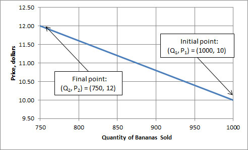
1) Using the original formula, we get:

$$\begin{array}{l}\eta =\left[\left(750–1000\right)/1000\right]/\left[\left(12-10\right)/10\right]\\ =-0.25/0.20=-1.25\end{array}$$

 

2) Using the midpoint formula, we get:

$$\begin{array}{l}\eta =\left[\left(750-1000\right)/\left(1000+750\right)\right]/\left[\left(12-10\right)/\left(10+12\right)\right]\\ =\left[250/1750\right]/\left[2/22\right]\\ =-0.1429/0.0909=-1.57\end{array}$$

 

So, these numbers are quite different.

What about the point elasticity? Well, to answer this, we need the slope of a line. If we assume that the demand curve is a straight line, then what is the slope? Given that we have the points (Q,P ) = (1000, 10) and (750, 12), then the slope is $\Delta P/\Delta Q$ = (12-10)/(750-1000) = -0.008. But in the elasticity, we need $\Delta Q/\Delta P$, which is -250/2 = -125.

So, at point 1, the point elasticity will be P/Q * $\Delta Q/\Delta P$= (10/1000) * -125 = -1.25. At point 2, it would be (12/750)*-125 = -2.

Steepness of Elasticity

If something only stretches a small amount under pressure, then we say it is inelastic. In economics, we say that a good is inelastic if its quantity demanded does not change very much with a change in price. On a supply and demand diagram, an inelastic good is one that has a very steep slope. This is shown in the following diagram:

Figure 2.5 Elasticities of various demand curves

Credit: Barry Posner

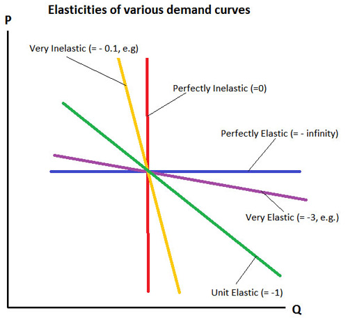
Typically, goods that are thought of as necessities will be very inelastic. That is, no matter how expensive they get, we will still buy them. Health care, staple foods and gasoline are goods with low elasticities. If a demand curve is perfectly vertical (up and down) then we say it is perfectly inelastic. If the curve is not steep, but instead shallow, then the good is said to be “elastic” or “highly elastic.” This means that a small change in the price of the good will have a large change in the quantity demanded. If the curve is perfectly flat (horizontal), then we say that it is perfectly elastic. Luxury goods are often very elastic – if the price increases a little, then people will move over to something else.

Remember that the elasticity is a ratio of percent changes in quantity and price.

Also, remember that all elasticities of demand will be negative, since the demand curve slopes downwards.

Summary

• A Perfectly Inelastic Demand Curve is vertical (η = 0). This is very rare in reality. You could claim that the elasticity of life-saving medical treatment is perfectly inelastic, since most of us would give anything and everything to stay alive.
• A highly inelastic demand curve is very steep (η close to zero, e.g., -0.1.) Many goods that are necessities or have very few substitutes behave this way.
• A demand curve with an elasticity near -1 is said to be “uniformly elastic.”
• A highly elastic demand curve is very flat (η between -2 and -5). Luxury goods, or goods with lots of substitutes behave like this.
  Perfectly elastic goods have a horizontal demand curve (η = -∞.) This is rare in the world.
• In the following diagram, the supposed value of the price elasticity of demand is shown beside each line.

Some sample elasticities (from the real world):

• Gasoline: -0.04
• Sugar: -0.31
• Long distance phone service (1995): 0.35
• Tires: -1.20
• Movies: -3.70

So, let's think for what these numbers mean. The elasticity of gasoline (or, if I want to be complete and formal, the price elasticity of demand of gasoline) is -0.04. Put another way, this means that if the price increases 1%, the quantity that the public wants to purchase only goes down 0.04%. Or if we scale these numbers up, we can say that if the price increases by 100% (that is, it doubles), then the quantity consumed only falls by 4%. So, if gasoline gets a lot more expensive, people will still use almost as much, at least in the short term. This is because most of us don't have a lot of choice about using gasoline (in the short term - more about what "short-term" means a bit later.) A lot of us don't have the option of using less gasoline, because we still need to get to the store and to work, and so on. Gasoline was more than twice as expensive in 2008 as it was in 2002, but we used about the same amount.

The number for long-distance phone service was also quite inelastic, because back in 1995 we didn't have a lot of options. Today, this number would be very different. Now we have cell phones that don't charge by how far you are from the caller, and we have Skype and we have VOIP and we have iPhones with video talk and we have webcams, and we have cable companies offering calling plans, and we have people talking about setting up communications networks on power lines, and so on.

Looking at the number for movies, we see that it has a high value (actually, because it is a negative number, it's actually smaller, but it is bigger in absolute terms.) This means that if the price goes up 1%, then the quantity demanded goes down by 3.4%. This is because movies are somewhat of a luxury, and there are usually plenty of alternatives.

We'll talk a lot more about the reasons behind these elasticities in Lesson 4 when we talk about market dynamics or what happens to supply and demand when we consider the effects of time and of the costs of other things. The important thing to take from this lesson is just to understand what a demand curve is, and how we measure just how much the quantity of a good demanded changes with the price of the good.

Reiteration

If you remember nothing else from this lesson, I hope you remember and understand the following two points.

1. A demand curve is a functional relationship. I cannot say this enough times. It is a curve that defines the relationship behind how much of a good will be demanded in a market at a certain price. Change the price, and a different quantity will be demanded. Demand is not a constant, but a variable.
2. Demand curves slope downwards because of the notion of declining marginal utility - the more of something that one has consumed, the less benefit (and, therefore, the less they are willing to pay) for the next unit of the good in question. Also, this is why the price elasticity of demand is negative: if price goes up, quantity demanded goes down, and vice versa.