Confidence Intervals and the Central Limit Theorem
 Read It: Confidence Intervals and the Central Limit Theorem
One application of the central limit theorem is finding confidence intervals. To do this, you need to use the following equation. Note that the z* value is not the same as the z-score described earlier, which was used to standardize the normal distribution. Here, the confidence interval is the sample statistic (e.g., , , etc.) plus/minus the z* value times the standard error. Note that this is the same equation we used in Lesson 4 when you learned about the standard error method. In Lesson 4, the z* value was set to 2 for the 95% confidence interval. This was an approximation of the z* value, which is actually 1.96 for an alpha value of 0.05.
where z* is chosen so that %P of the distribution is between -z* and +z* for %P confidence level.
The z* value, therefore, is only dependent on the confidence level. In other words, if you consider two very different datasets, the sample statistic and standard error will change, but the z* value will remain the same as long as you are using the same confidence level for both datasets. These z* values can be found in tables that list the values for a given alpha level, making it easy to quickly find different confidence intervals for the different levels. For example, for a 99% confidence interval, shown below, the z* value is 2.576. The confidence interval could then be calculated by plugging that value into the above equation, along with the sample statistic and standard error.
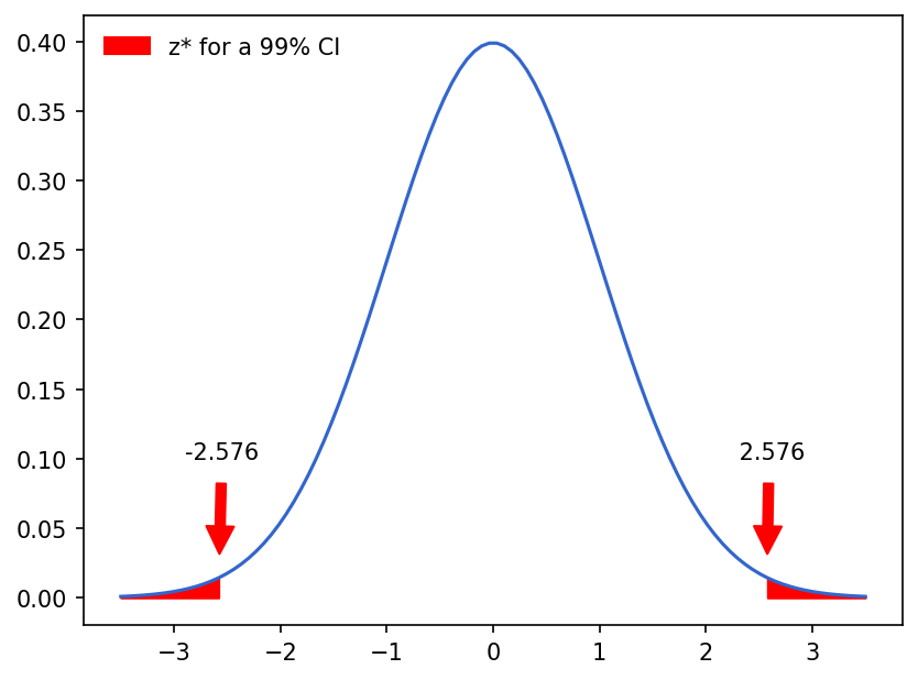
Example of a 99% confidence interval calculated using the z* value.
 Watch It: Video - Confidence Interval from Normal Distribution (5:32 minutes)
All right, we're going to continue to talk about the normal distribution in this video. And in particular, we're going to learn how to actually calculate the confidence interval from the normal distribution. And so, in the past we have defined our 95 percent confidence interval as the mean, plus or minus the two times the standard deviation. And so, in effect that looked something like using our data from above where we calculated the mean and standard error of our p hat distribution, meanR minus 2 times SER comma meanR plus 2 times SER. Then we can print the confidence interval. And so, here we can see that the 95 percent confidence interval is 0.37 to 0.63. But this is an approximation. Normally our value here, is usually calculated from something known as a z star, z, or a z statistic. So in order to do that, we need to specify the interval, P equals 95. And then we calculate the zstar which is just using stats dot norm dot interval of P divided by 100. And what we want to do is convert this into an array so we can run that. We can look at zstar which is minus 1.95 plus 1.95. And we can see how that is very close to 2. So what we have been doing so far in this class is using two as a very easy approximation for the actual z-star value, which is 1.95996398. So if we want to do a confidence interval with this zstar, we can really use the same formula. I'm going to copy this down. But instead of 2, we can use the actual value. So, and we don't need to do an array because this value already has the negative and the positive here. So I'm going to erase that, still say meanR but replace 2 with zstar times the standard error for R. And so, we can run this. And we can see that it has flipped it until we do this, change this to a plus. It goes back to the order, smaller versus larger because that's adding a negative and then adding a positive. And so we can see that it actually is very similar once it gets out to this third digit is where we start to see differences in the confidence interval. But the benefit to doing this type of methodology is that we can easily change our confidence interval to whatever confidence level we want by just changing this p-value. So if we want the 80th confidence interval, all I need to do is change that to 80. My zstar changes and now my confidence interval has changed. And so, this is a very easy way to do confidence intervals. And it's something that you would normally do in a traditional statistics class where you would look up this zstar value or your dip in confidence level and do a calculation. But it's important to note that this style of doing confidence intervals assumes that your data is normally distributed, and that it is sufficiently large enough to do this type of statistical analysis on it because it is following the central limit theorem, which we talked about earlier in the lesson.
 Try It: DataCamp - Apply Your Coding Skills
Try to find the 99% confidence interval of the 'phatdf' dataframe using the z* method discussed above.
 Assess It: Check Your Knowledge