Lessons
This is the course outline.
Lesson 1: Investment Decision Making and Compound Interest
Introduction
Overview
This course deals with mineral and oil project evaluation and investment decision-making. We will start by introducing the process of investment decision-making and the compound interest rate method. To make an investment decision, one needs to experience the processes of defining the problem, analyzing the problem, developing alternative solutions, deciding upon the best solution and converting the decision into effective action.
Then, in Lesson 1, the compound interest rate will be covered. Using the compounding method, we can select the appropriate factors to calculate the future value, current value, and the annual value.
One goal of this course is the application of project evaluation methods in the mining and oil industry. Besides the evaluation techniques, this lesson will cover some background and knowledge about the mining and oil industries, through readings of news and papers.
Learning Objectives
At the successful completion of this lesson, students should:
- understand the processes of investment decision-making;
- understand how to use compounding interest rates to calculate present, future, and annual values;
- understand how to apply the evaluation techniques in the mining and oil industry; and
- understand how to use Microsoft Excel for the calculations.
What is due for Lesson 1?
| Reading | Chapter 1 of the textbook by Stermole. |
|---|---|
| Assignment |
Go through the Syllabus, Orientation, and Lesson 1 on the website. |
Questions?
If you have any questions, please post them to the discussion forum, located under the Modules tab in Canvas. The TA and I will check that discussion forum daily to respond. While you are there, feel free to post your own responses if you, too, are able to help out a classmate.
Introduction to Investment Analysis
Investors make decisions relying on the relative profit potential of investment alternatives. The wrong choices may be made if systematic and quantitative methods are not used. In a given investment situation, it is necessary to consider several economic and technical parameters with respect to costs, profits, savings, the choice of time, tax and loyalty, project life, etc. If a reliable approach is not used to quantify the effects of these factors, it is very difficult to correctly assess each alternative and make the best choice.
The economic viewpoint assumes that capital accumulation is the primary investment objective of capitalistic individuals, companies and societies. From the late 1980s to the late 1990s, it is estimated that more capital investment dollars were spent in the US than were spent cumulatively in the past 200 years in the US. And the numbers in the 2010s were even larger. The importance of proper economic evaluation techniques in determining the most economically-effective way to spend this money seems evident for individuals, companies, and societies. This course presents the development and application of these economic evaluation techniques.
Investment decisions are analyzed over the lifetime of a project which can be decades long, and there are many input data that are related to time such as escalation and inflation of costs and revenues. Therefore, predictions, forecasting, estimations, and assumptions are required for these data which is involved with risk and uncertainty. Consequently, results of the analysis are highly dependent on accuracy and correctness of the proposed inputs. However, the techniques provided in this text can give the decision maker much better ideas about the relative risks and uncertainties between alternatives. This information, along with the numerical economic evaluation results, can help the investors to make a better choice than without using them.
In the majority of cases, making business decisions means dealing with alternative choice problems, which includes selecting the best alternative from several possible choices. The economic evaluation techniques in this course are based on the premise that profit maximization is the investment objective; that is, the alternation that maximizes the future worth of available investment dollars. In general, this involves answering the question, “Is it better to invest cash in a given investment situation, or will the cash earn more if it is invested in an alternative situation?”
Several applicable and useful techniques for evaluating various investment situations will be covered in this course and include future, present, annual value, and break-even analysis. But, the course focuses mainly on methods such as compound interest rate of return (ROR) analysis, as the primary decision-making criterion used by the majority of firms and organizations, and net present value (NPV) analysis, as the second-most used technique, properly applied on an after-tax basis.
Taxes are a cost relevant to most evaluation situations and economic analysis must be done after-tax. This course will cover the scenarios that it is proper to neglect taxes such as government project evaluations where taxes do not apply. Also, the cases with taxes incorporated will also be discussed and analyzed.
There are two main categories of projects or investments that economic evaluation decision-making can be applied to:
- revenue producing investments
- service producing investments
A possible third classification, “saving producing projects” will be illustrated later in the course.
Discounting and Compounding
Compounding
In order to compare different alternatives in an economic evaluation, they should have the same base (equivalent base). Compound interest is a method that can help applying the time value of money. For example, assume you have 100 dollars now and you put it in a bank for interest rate of 3% per year. After one year, the bank will pay you . Then, you will put the 103 dollars in the bank again for another year. One year later, you will have . If you repeat this action over and over, you will have:
Which can be written as:
In general:
The value of money after nth period of time can be calculated as:
Which F is the future value of money, P is the money that you have at the present time, and i is the compound interest rate.
Example 1-1:
Assume you put 20,000 dollars (principal) in a bank for the interest rate of 4%. How much money will the bank give you after 10 years?
So the bank will pay you 29604.8 after 10 years.
Discounting
In economic evaluations, “discounted” is equivalent to “present value” or “present worth” of money. As you know, the value of money is dependent on time; you prefer to have 100 dollars now rather than five years from now, because with 100 dollars you can buy more things now than five years from now, and the value of 100 dollars in the future is equivalent to a lower present value. That's why when you take loan from the bank, the summation of all your installments will be higher than the loan that you take. In an investment project, flow of money can occur in different time intervals. In order to evaluate the project, time value of money should be taken into consideration, and values should have the same base. Otherwise, different alternatives can’t be compared.
Assume you temporarily worked in a project, and in the end (which is present time), you are offered to be paid 2000 dollars now or 2600 dollars 3 years from now. Which payment method will you chose?
In order to decide, you need to know how much is the value of 2600 dollars now, to be able to compare that with 2000 dollars. To calculate the present value of a money occurred in the future, you need to discount that to the present time and to do so, you need discount rate. Discount rate, i, is the rate that money is discounted over the time, the rate that time adds/drops value to the money per time period. It is the interest rate that brings future values into the present when considering the time value of money. Discount rate represents the rate of return on similar investments with the same level of risk.
So, if the discount rate is i=10% per year, it means the value of money that you have now is 10% higher next year. So, if you have P dollars money now, next year you will have and if you have F dollars money next year, your money is equivalent to dollars at present time.
Going back to the example, considering the discount rate of 10%:
We can calculate the present value of $2600 occurred 3 years from now by discounting it year by year back to the present time:
Value of 2600 dollars in the 2nd years from now
Value of 2600 dollars in the 1st years from now
Value of 2600 dollars at the present time
So, it seems at the discount rate of i=10%, present value of 2600 dollars in 3 years equals 1953.42 dollars, and you are better off, if you accept the 2000 dollars now.
With the following fundamental equation, present value of a single sum of money in any time in the future can be calculated. It means a single sum of money in the future can be converted to an equivalent present single sum of money, knowing the interest rate and the time. This is called discounting.
P: Present single sum of money.
F: A future single sum of money at some designated future date.
n: The number of periods in the project evaluation life (can be year, quarter or month).
i: The discount rate (interest rate).
Example 1-2:
Assuming the discount rate of 10 %, present value of 100 dollars which will be received in 5 years from now can be calculated as:
You can see how time and discount rate can affect the value of money in the future. 62.1 dollars is the equivalent present sum that has the same value of 100 dollars in five years under the discount rate of 10%
Note:
The concept of compounding and discounting are similar. Discounting brings a future sum of money to the present time using discount rate and compounding brings a present sum of money to future time.
Compound Interest Formulas I
Example 1-2 was about one single sum; what if you want to add some savings to your bank account each year? So, we need to learn some more techniques to be prepared for real-world economic evaluations. First, take a look at Figure 1-2. It can help us to better understand the investment evaluation problems.
| P | A | A | A | A | A | F | ||
|
|
||||||||
| 0 | 1 | 2 | 3 | ... | n-1 | n | ||
Figure 1-2: Time diagram
The horizontal line represents the time. The left-hand end shows the present time and the right-hand end shows the future. The numbers below the line (1, 2, 3, …, n) are time periods. Above each time period, there is a sum A, which shows the money that occurs in that time period; here, we assume all of them are equal payments, so:
A is a uniform series of equal payments at each compounding period;
P is a present single sum of money at the time zero;
F is a future sum of money at the end of period n. And i is the compound interest rate.
In order to understand an economic evaluation problem we have to determine:
- How much money is given?
- When is the money given (where on the timeline)?
- What is the time period (year, quarter, or month)?
- What is the interest rate?
- What needs to be calculated?
Following these steps, we just need to use the proper equation to solve the problem. Based on the unknown (asked) variable, there are six basic categories of problems here:
- F (future value) needs to be calculated from given P
- F (future value) needs to be calculated from given A
- P (present value) needs to be calculated from given F
- P (present value) needs to be calculated from given A
- A (uniform and equal period values) needs to be calculated from given F
- A (uniform and equal period values) needs to be calculated from given P
Table 1-1 displays a method of notation that can help summarize the given information and avoid confusion.
| To be Calculated Quantity | Given Quantity | Appropriate Factor (symbol) | Relationship | |
|---|---|---|---|---|
| 1 | F | P | ||
| 2 | P | F | ||
| 3 | F | A | ||
| 4 | A | F | ||
| 5 | P | A | ||
| 6 | A | P |
Note: “/” in the Appropriate Factor (symbol) column is not a division operator, the entire or , … is a factor (symbol). The first letter shows the variable that needs to be calculated and the second letter shows the given variable. The two subscripts on each factor are the given period interest rate, i, followed by the number of interest compounding periods, n.
The new notation helps us summarize the problem. The factor actually give a gives us a coefficient that when multiplied by given parameter, gives the unknown parameter.
All time value of money calculations involves writing an equation or equations to calculate F, P, or A. Each of terms in the column “Appropriate Factor (symbol)” has a name that you will learn later in this course.
Please watch the following (4:32) video:
PRESENTER: Hello. In this video, I'm going to summarize the basic economic evaluation problems, and I will explain how to approach each one. When facing a problem, we have to ask these five main questions. How much money is given? When is the money given, or where on the timeline? What is the time period, year, quarter, or month? What is the interest rate? What needs to be calculated?
The next step in approaching the problem is to draw the timeline. Here, as you can see, the horizontal line represents the time. The left hand end shows the present time and right hand end shows the future. Numbers below the line 0, 1, 2, 3, and n are time periods.
Now, let's add the variables. P on the left hand side is the present single sum of money at time zero. This is the amount of money that is received or paid at the present time, at time zero, at year zero or month zero. We could also write it-- write this P above the time zero. It would be the same.
The other variable is F, which is the future sum of money at the end of the period n. This is the amount of money that is received or paid in the future in the end of the end period, end year, end month. We could also write it above the end year, it's the same. The other parameter is A.
Above each time period starting from year one to year n, there is an A, which are called uniform series of equal payments at each compounding period. These A's show the money that has occurred, that is paid or received in those time periods. Here we assume all of them are equal payments.
When we face a problem, we just need to use the proper equation to solve it. And the next step is to figure out what type of problem we have. Based on given and unknown variables, there are six main categories of problems. In first category, P, money paid or received at the present time is given, and F, future value of that amount needs to be calculated.
Second category, F is given and P needs to be calculated. In third category, F needs to be calculated from given A, uniform and equal series of payments. In fourth category, A needs to be calculated from given f. Fifth category, P, present value, needs to be calculated from given A, and in sixth category, a needs to be calculated from given P. Note that in each type, we have only two money variables.
You can see these six categories in this table. The first column shows the unknown variable, the variable that needs to be calculated. The second column shows the given variable. And the third column shows the appropriate factor. Factor is just a notation, a symbol to summarize the problem.
The slash sign is not a division operator. The first letter on the left hand side of the slash sign shows the variable that needs to be calculated. And the second letter on the right hand side of the slash sign shows the given variable. The two subscripts on each factor are period interest rate, i, followed by the number of interest compounding period, n.
1. Single Payment Compound-Amount Factor
The first category of six categories that were introduced explains the situation that the present value of money is given and asks you to calculate the future value according to the given interest rate of i per period and n period from now. This problem can be summarized with the factor (symbol) of and can be shown as:
| P | _ | _ | _ | _ | _ | F=? | ||
|
|
||||||||
| 0 | 1 | 2 | 3 | ... | n-1 | n | ||
Figure 1-3: Single Payment Compound-Amount Factor, F/Pi,n
As explained earlier, the future value of money after n period with an interest rate of i can be calculated using the Equation 1-1: which can also be written regarding Table 1-1 notation as: . The mathematical expression is called the “single payment compound-amount factor."
Compound Interest Formulas II
3. Uniform Series Compound-Amount Factor
The third category of problems in Table 1-5 demonstrates the situation that equal amounts of money, A, are invested at each time period for n number of time periods at interest rate of i (given information are A, n, and i) and the future worth (value) of those amounts needs to be calculated. This set of problems can be noted as . The following graph shows the amount occurred. Think of it as this example: you are able to deposit A dollars every year (at the end of the year, starting from year 1) in an imaginary bank account that gives you i percent interest and you can repeat this for n years (depositing A dollars at the end of the year). You want to know how much you will have at the end of year nth.
| 0 | A | A | A | A | F=? | ||
|
|
|||||||
| 0 | 1 | 2 | ... | n-1 | n | ||
Figure 1-4: Uniform Series Compound-Amount Factor,
In this case, utilizing Equation 1-2 can help us calculate the future value of each single investment and then the cumulative future worth of these equal investments.
Future value of first investment occurred at time period 1 equals
Note that first investment occurred in time period 1 (one period after present time) so it is n-1 periods before the nth period and then the power is n-1.
And similarly:
Future value of second investment occurred at time period 2:
Future value of third investment occurred at time period 3:
Future value of last investment occurred at time period n:
Note that the last payment occurs at the same time as F.
So, the summation of all future values is
By multiplying both sides by (1+i), we will have
By subtracting first equation from second one, we will have
which becomes:
then
Therefore, Equation 1-3 can determine the future value of uniform series of equal investments as . Which can also be written regarding Table 1-5 notation as: . Then .
The factor is called “Uniform Series Compound-Amount Factor” and is designated by F/Ai,n. This factor is used to calculate a future single sum, “F”, that is equivalent to a uniform series of equal end of period payments, “A”.
Note that n is the number of time periods that equal series of payments occur.
Please review the following video, Uniform Series Compound-Amount Factor (3:42).
PRESENTER: In the third category, equal amounts of money A are enlisted pay to receive at each time period for n number of time periods. n can be years or months, and interest rate is i. And the question asks you to calculate the future value of these payments, a single sum of money that is equivalent to all these series of payments A. Here, given information are A, n, and i. And F is the unknown parameter. These sets of problems can be displayed with the factor F slash A, or F/A. Again, the left side of this slash sign is the unknown parameter F, and the right side is the given variable, which is A.
Here, you can see the equation to calculate F from A, i and n. The mathematical proof of this equation is straightforward, and they explain it in Lesson One. We can write this equation, regarding the factor notation, F equals A multiply the factor. This factor is called uniform series compound-amount factor. And it is used to calculate the future single sum F that is equivalent to uniform series of equal ends of period payments A.
Let's work on an example to see how this factor can be used. Assume you save $4,000 per year and deposit it, in the end of the year, in an imaginary saving account or some other investment that gives you 6% interest rate per year, compounded annually, for 20 years, starting from year 1 to year 20th. And you want to know how much money will you have in the end of the 20th year.
First, we draw the time line. Left-hand side is the present time. We don't have anything there. Note that your investment, it starts from year 1 to year 20th. If there is no extra information in the question, and question says you invest for 20 years, you need to assume your investment, it starts from year 1. So there is no payment at present time, or year zero.
Right-hand side is the future time, which is a single amount future value, and it is unknown. Your investment takes 20 years, so n equals 20. And above each year, you have to write $4,000, because you have a payment of $4,000 in the end of each year. So A equals $4,000, n number of years is 20, i interest rate 6%, and F needs to be calculated.
And F equals A times the factor F/A. In this factor, i is 6% and 20. And we use the equation to calculate the F. And we find the answer. So if you invest $4,000 per year for 20 years, with 6% interest rate, you will have about $147,000 at the end of the 20th year.
Example 1-3:
Assume you save 4000 dollars per year and deposit it at the end of the year in an imaginary saving account (or some other investment) that gives you 6% interest rate (per year compounded annually), for 20 years. How much money will you have at the end of the 20th year?
| 0 | $4000 | $4000 | $4000 | $4000 | F=? | ||
|
|
|||||||
| 0 | 1 | 2 | ... | 19 | 20 | ||
So
A =$4000
n =20
i =6%
F=?
Please note that n is the number of equal payments.
Using Equation 1-3, we will have
So, you will have 147,142.4 dollars at 20th year.
| Factor | Name | Formula | Requested variable | Given variables |
|---|---|---|---|---|
| F/Ai,n | Uniform Series Compound-Amount Factor | F: Future value of uniform series of equal investments | A: uniform series of equal investments n: number of time periods i: interest rate |
4. Sinking-Fund Deposit Factor
The fourth group in Table 1-5 is similar to the third group but instead of A as given and F as unknown parameters, F is given and A needs to be calculated. This group illustrates the set of problems that ask you to calculate uniform series of equal payments (or investment), A, to be invested for n number of time periods at interest rate of i and accumulated future value of all payments equal to F. Such problems can be noted as and are displayed in the following graph. Think of it as this example: you are planning to have F dollars in n years and there is a saving account that can give you i percent interest. You want to know how much you have to deposit every year (at the end of the year, starting from year 1) to be able to have F dollars after n years.
| 0 | A=? | A=? | A=? | A=? | F | ||
|
|
|||||||
| 0 | 1 | 2 | ... | n-1 | n | ||
Figure 1-5: Sinking-Fund Deposit Factor,
Equation 1-3 can be rewritten for A (as unknown) to solve these problems:
Equation 1-4 can determine uniform series of equal investments, A, given the cumulated future value, F, the number of the investment period, n, and interest rate i. Table 1-5 notes these problems as: . Then . The factor is called the “sinking-fund deposit factor”, and is designated by . The factor is used to calculate a uniform series of equal end-of-period payments, A, that are equivalent to a future sum F.
Note that n is the number of time periods that equal series of payments occur.
Please watch the following video, Sinking Fund Deposit Factor (4:42).
PRESENTER: The fourth group is similar to the third one. But A is the unknown and F is the given variable. This set of problems asks you to calculate uniform series of equal payments, A, to be invested for n number of time periods at interest rate of i. And the accumulated future value of all payments or equivalent future value is F.
This set of problems can be summarized with the factor A over F or A slash F. The left side of this last sign is the unknown parameter. Here it is A. And the right side is the given variable, which is F.
Equation 1-3 for uniform series compound amount factor can be rewritten for A as unknown to solve these problems, which gives the Equation 1-4. Equation 1-4 can determine uniform series of equal investments, A, for accumulated future value, F, number of investment period n and interest rate i.
We can write this equation according to the factor notation, A equals F times the factor A over F. This factor is called the Sinking-Fund Deposit Factor. And it is displayed by A slash F. The factor is used to calculate the uniform series of equal end of the period payments, A, that are equivalent to a future sum, F.
For example, referring to example 1-7 in previous video, let's say you plan to have $200,000 after 20 years. And you are offered an investment, which can be the imaginary savings account, that gives you 6% per year compound interest rates. And you want to know how much money, equal payments, you need to save each year, or invest-- deposit in your account in the end of each year.
So in summary, you want to have $200,000 after 20 years. And you can invest your money with 6% interest rate. The question is, how much you need to invest per year?
Again, the first step is drawing the time line. Left-hand side is the present time. We won't have any payment. So there is no payment at present time or time zero. Right-hand side is the future. And you want to have a single amount of $200,000. So you write $200,000 in the 20th year, or in the end of right-hand side of the time line.
Note that $200,000 has the same time dimension as the last payment, A. Both are in the year 20th. Your investment takes 20 years, so n equals 20. And above each year, you have to write A, which is unknown and needs to be calculated.
So F equals $200,000. n number of years is 20. i, interest rate, 6%. And A needs to be calculated.
We can use the factor notation to summarize the equation. In this factor, i is 6%, n is 20, and F is given, and A needs to be calculated. And we calculate the result. So if you want to have $200,000 in 20 years from now with 6% interest rate, you will need to invest equal amounts of $5,437 per year at the end of each year for 20 years, starting from year one.
Example 1-4:
Referring to Example 1-3, assume you plan to have 200,000 dollars after 20 years, and you are offered an investment (imaginary saving account) that gives you 6% per year compound interest rate. How much money (equal payments) do you need to save each year and invest (deposit it to your account) in the end of each year?
| 0 | A=? | A=? | A=? | A=? | F=200,000 | ||
|
|
|||||||
| 0 | 1 | 2 | ... | 19 | 20 | ||
So
F=$200,000
n=20
i=6%
A=?
Using Equation 1-4, we will have
So, in order to have 200,000 dollars at 20th year, you have to invest 5,436.9 dollars in the end of each year for 20 years at annual compound interest rate of 6%.
| Factor | Name | Formula | Requested variable | Given variables |
|---|---|---|---|---|
| Sinking-Fund Deposit Factor | A: Uniform series of equal end-of-period payments | F: cumulated future value of investments n: number of time periods i: interest rate |
Note that
Compound Interest Formulas III
5. Uniform Series Present-Worth Factor
The fifth group in Table 1-5 covers a set of problems that uniform series of equal investments, A, occurred at the end of each time period for n number of periods at the compound interest rate of i. In this case, the cumulated present value of all investments, P, needs to be calculated. In summary, P is unknown and A, i, and n are given parameters. And the problem can be noted as and displayed as:
| P=? | A | A | A | A | 0 | ||
|
|
|||||||
| 0 | 1 | 2 | ... | n-1 | n | ||
Figure 1-6: Uniform Series Present-Worth Factor,
If we replace substitute F in Equation 1-3 from Equation 1-2, we will have the present value as:
then,
Equation 1-5 gives the cumulated present value, P, of all uniform series of equal investments, A, as . And also can be noted as: .The factor is called the “uniform series present-worth factor” and is designated by . This factor is used to calculate the present sum, P that is equivalent to a uniform of equal end of period payments, A. Then
Note that n is the number of time periods that equal series of payments occur.
Please review the following video, Uniform Series Present Worth Factor (Time 3:35).
PRESENTER: The fifth group covers the set of problems that P is a known parameter, A, i and n are given variables. In these problems, we have uniform series of equal investments, A, in the end of each time period, for n number of periods, at the compound interest rate of I.
And the problem asks you to calculate the accumulated present value of all investments, P. We can summarize these questions using the factor notation. P is the unknown variable, and should be on the left side. And A is the given, and should be written on the right side.
As explained before, Equation 1-3 returns the future value, F, from A, i and n. And Equation 1-2 calculates the future value, F, from present value, P, interest rates, i and n number of periods. So if we substitute F in Equation 1-3 from Equation 1-2, we will have this new equation-- 1-5. This equation gives us the accumulated present value of equal series payments, A, paid for n period, at interest rate of i.
Equation 1-5 can also be written according to factor notation. P equals A times the factor P over A. This factor is called Uniform Series Present-Worth Factor, which is used to calculate the presence on P that is equivalent to a uniform series of equal payments, end of the period payments, A.
For example, what would be the present value of 10 uniform investments of $2,000, invested at the end of each year, for interest rate of 12%, compounded annually? First, we draw the time line. Left hand side is a present time, time zero payment, which needs to be calculated. N equals 10, because there are 10 uniform investments.
So we have 10 years. And above each year, we have $2,000, starting from year one to year 10. So A equals $2,000, n is 10, and interest rate is 12%. Using the factorization, P equals A, multiply the factor-- i is 12%, and n is 10. And the result.
So if you save $2,000 per year, at the end of each year for 10 years, starting from year one to year 10, the accumulated money is equal to $11,300 at present time. It has the same value as $11,300 at the present time.
Example 1-5:
Calculate the present value of 10 uniform investments of 2000 dollars to be invested at the end of each year for interest rate 12% per year compound annually.
| P=? | A=$2000 | A=$2000 | A=$2000 | A=$2000 | 0 | ||
|
|
|||||||
| 0 | 1 | 2 | ... | 9 | 10 | ||
So,
A =$2000
n =10
i =12%
P=?
Using Equation 1-5, we will have:
Note that we use the factor when we have equal series of payments. i is the interest rate and n is the number of equal payments. There is an important assumption here, the first payment has to start from year 1. In that case will return the equivalent present value of the equal payments.
Now let's consider the case that we have equal series of payments and the first payment doesn't start from year 1. In that case the factor will give us the equivalent single value of equal series of payments in the year before the first payment. However, we want the present value of them (at year 0). So, we need to multiply that with the factor and discount it to the present time (year 0).
Example:
| P=? | A=$2000 | A=$2000 | A=$2000 | 0 | |||
|
|
|||||||
| 0 | 1 | 2 | ... | 10 | 11 | ||
Note that there are 10 equal series of $2,000 payments. But the first payment is not in year 1. The factor returns the equivalent value of these 10 payments to the year before the first payment, which is year 1.
| P=? | $2000(P/A12%,10) | 0 | |||||
|
|
|||||||
| 0 | 1 | 2 | ... | 10 | 11 | ||
However, we want the present value. So, we need to discount the value by one year to have the present value of 10 equal payments.
| P=? | $2000(P/A12%,10)(P/F12%,1) | 0 | |||||
|
|
|||||||
| 0 | 1 | 2 | ... | 10 | 11 | ||
Example: Now consider the the following case that the first payment starts at year 3:
| P=? | A=$2000 | A=$2000 | A=$2000 | 0 | ||||
|
|
||||||||
| 0 | 1 | 2 | 3 | ... | 10 | 12 | ||
| Factor | Name | Formula | Requested variable | Given variables |
|---|---|---|---|---|
| Uniform Series Present-Worth Factor | P: Present value of uniform series of equal investments | A: uniform series of equal investments n: number of time periods i: interest rate |
6.Capital-Recovery Factor
The sixth group in Table 1-5 belongs to set of problems that A is unknown and P, i, and n are given parameters. In this category, uniform series of an equal sum, A, is invested at the end of each time period for n periods at the compound interest rate of i. In this case, the cumulated present value of all investments, P, is given and A needs to be calculated. It can be noted as .
| P | A=? | A=? | A=? | A=? | 0 | ||
|
|
|||||||
| 0 | 1 | 2 | ... | n-1 | n | ||
Figure 1-7: Capital-Recovery Factor,
Equation 1-5 can be rewritten for A (as unknown) to solve these problems:
Equation 1-6 determines the uniform series of equal investments, A, from cumulated present value, P, as . The factor is called the “capital-recovery factor” and is designated by A/Pi,n. This factor is used to calculate a uniform series of end of period payment, A that are equivalent to present single sum of money P.
Note that n is the number of time periods that equal series of payments occur.
Please watch the following video, Capital Recovery Factor (Time 3:37).
PRESENTER: The sixth group belongs to the set of problems that A is unknown and P, i, and n are given parameters. This category is similar to the fifth group, but P is given and A needs to be calculated. In this category of problems, we know the present value P, or accumulated present value of all payments. And we want to calculate the uniform series of equal sum A that are invested in the end of each time period for n periods at the compound interest rate of i.
So we have present value P, and we want to calculate equivalent A, given interest rate of i and number of periods n. The proper factor to summarize these questions is A over P, or A/P. A is the unknown variable, is on the left side, and P, given variable, on the right side.
Equation to calculate A is straightforward. We just need to rewrite the equation in 1-5 for A as unknown, and we will have equation 1-6 that calculates A from P, i, and n. If we write the equation 1-6 according to the factor notation, we will have factor A over P. The factor is called capital recovery factor and is used to calculate uniform sales of end of period payments A that are equivalent to present single sum of money P.
Let's work on this example. We want to know the uniform series of equal investment for five years at interest rate of 4% which are equivalent to $25,000 today. Let's say you want to buy a car today for $25,000, and you can finance the car for five years and 4% of interest rate per year, compounded annually. And you want to know how much you have to pay each year.
First, we draw the timeline. Left side is the present time, which we have $25,000. n equals 5, and above each year, starting from year one to year five, we have A that has to be calculated. For the factor, we have i equal 4% and n is five and the result, which tells us $25,000 at present time is equivalent to five uniform payments of $5,616 starting from year one to year five with 4% annual interest rate. Or $25,000 at present time has the same value of five uniform payments of $5,616 starting from year one to year five with 4% annual interest rate.
Example 1-6:
Calculate uniform series of equal investment for 5 years from present at an interest rate of 4% per year compound annually which are equivalent to 25,000 dollars today. (Assume you want to buy a car today for 25000 dollars and you can finance the car for 5 years with 4% of interest rate per year compound annually, how much you have to pay each year?)
| P=$25,000 | A=? | A=? | A=? | A=? | A=? | 0 | |
|
|
|||||||
| 0 | 1 | 2 | 3 | 4 | 5 | ||
Using Equation 1-6, we will have:
So, having $25,000 at the present time is equivalent to investing $5,615.68 each year (at the end of the year) for 5 years at annual compound interest rate of 4%.
| Factor | Name | Formula | Requested variable | Given variables |
|---|---|---|---|---|
| Capital-Recovery Factor | A: uniform series of equal investments | P: Present value of uniform series of equal investments n: number of time periods i: interest rate |
Note that
Using these six techniques, we can solve more complicated questions.
Example 1-7:
Assume a person invests 1000 dollars in the first year, 1500 dollars in the second year, 1800 dollars in the third year, 1200 dollars in the fourth year and 2000 dollars in the fifth year. At an interest rate of 8%:
1) Calculate time zero lump sum settlement “P”.
2) Calculate end of year five lump sum settlement “F”, that is equivalent to receiving the end of the period payments.
3) Calculate five uniform series of equal payments "A", starting at year one, that is equivalent to above values.
| P=? | 1000 | 1500 | 1800 | 1200 | 2000 | F=? | |
|
|
|||||||
| 0 | 1 | 2 | 3 | 4 | 5 | ||
1) Time zero lump sum settlement “P” equals the summation of present values:
2) End of year five lump sum settlement “F”, that is equivalent to receiving the end of the period payments equals the summation of future values:
Please note that in the factor subscript, n is the number of time period difference between F (the time that future value has to be calculated) and P(the time that the payment occurred). For example, 1800 payment occurs in year 3 but we need its future value in year 5 (2 year after) and time difference is 2 years. So, the proper factor would be: .
3) Uniform series of equal payments "A" can be calculated from either P or F :
or
Example 1-8: repeat your calculations for the following payments:
| P=? | 800 | 1000 | 1000 | 1600 | 1400 | F=? | |
|
|
|||||||
| 0 | 1 | 2 | 3 | 4 | 5 | ||
1) Time zero lump sum settlement “P” equals the summation of present values:
2) End of year five lump sum settlement “F”, that is equivalent to receiving the end of the period payments equals the summation of future values:
3) Uniform series of equal payments "A" can be calculated from either P or F:
or
Cash Flow
The first step in conducting an economic evaluation analysis is to understand the concept of “cash flow.” “Cash flow” represents the net inflow or outflow of money during a given period of time that can be month, quarter, or year. Cash flow can be reported as before-tax cash flow (BTCF) and after-tax cash flow (ATCF).
Operating Profit or EBITDA = Gross Revenue or Savings – Operating Expenses
Before tax Cash Flow = Operating Profit or EBITDA – Capital Expenditure
After tax Cash Flow = Before tax Cash Flow – Income Tax Expenditure
Which is formatted as:
Gross Revenue or Savings
– Operating Expenses
_____________________________
Operating Profit or EBITDA
– Capital Expenditure
_____________________________
Before tax Cash Flow
– Income Tax Expenditure
_____________________________
After tax Cash Flow
EBITDA : Earnings before interest, taxes, depreciation, and amortization
Example 1-9:
Assume an investment project for which you need to invest 20 and 15 million dollars in year 0 and year 1 (you can think of it as 20 million dollars now and 15 million dollars next year) to build a facility. In year 2, the plant will start producing and you can make revenue by selling the products. Each year, starting from year 2, operating costs and tax have to be paid. Project net cash flow can be calculated as:
| Year 0 | Year 1 | Year 2 | Year 3 | Year 4 | Year 5 | Year 6 | Year 7 | Year 8 | |
|---|---|---|---|---|---|---|---|---|---|
| Revenue | 18 | 20 | 22 | 24 | 26 | 28 | 30 | ||
| Operating Cost | -4 | -4 | -4 | -5 | -6 | -8 | -10 | ||
| Capital Cost | -20 | -15 | |||||||
| Tax Cost | -3 | -4 | -5 | -6 | -7 | -8 | -9 | ||
| Project Cash Flow | -20 | -15 | 11 | 12 | 13 | 13 | 13 | 12 | 11 |
Each column stands for a time period (that can be year, quarter, month, …) and each cell shows the inflow or outflow of money. Investment cash flow in any year represents the net difference between inflows of money from all sources, minus investment outflows of money from all sources. The cash flow for this project for all years is calculated in the last row.
As you can see, all the costs (Capital Cost, Operating Cost, Tax, ...) are entered with the negative sign in the table, and then summation of each column gives the net cash flow in that year. The negative cash flow incurred in years 0 and 1 will be paid off by positive cash flows in years 2 through 8.
Discounted Cash Flow (DCF)
If future cash flow is discounted, we can have cash flow in terms of present value, which is called discounted cash flow (DCF). As explained before, DCF considers the time value of money and applies it to the inflow and outflow of money occurred in the future. DCF is a tool that enables us to compare the future cash flow with the present value of money.
Different investment projects have different cash flows that happen in different time intervals in the future and DCF can give an assessment to decide which project is more profitable. DCF brings the future amounts to a same base that is easily understandable for decision makers. For example, assume you have two options: investing your money in Project A that gives you 1000 dollars every year from 2025 to 2035 or investing in Project B that gives you 1500 dollars every year from 2030 to 2040. Which project will you choose? DCF is a tool that can help you finding the answer. DCF can also be used to estimate the value of a company based on its future performance.
Example 1-10:
Please calculate the discounted cash flow from Example 1-9 assuming:
1) Discount rate = 10%
2) Discount rate = 12%
3) Discount rate = 15%
Assuming discount rate = 10%:
We can repeat the same procedure for discount rate = 12% and 15%. Table 1-2 shows the results.
| Year | 0 | 1 | 2 | 3 | 4 | 5 | 6 | 7 | 8 |
|---|---|---|---|---|---|---|---|---|---|
| Project Cash Flow | -20 | -15 | 11 | 12 | 13 | 13 | 13 | 12 | 11 |
| DCF (discount rate = 10%) | -20 | -13.6 | 9.1 | 9.0 | 8.9 | 8.1 | 7.3 | 6.2 | 5.1 |
| DCF (discount rate = 12%) | -20 | -13.4 | 8.8 | 8.5 | 8.3 | 7.4 | 6.6 | 5.4 | 4.4 |
| DCF (discount rate = 15%) | -20 | -13 | 8.3 | 7.9 | 7.4 | 6.5 | 5.6 | 4.5 | 3.6 |
Net Present Value (NPV)
Now, all the DCFs in Table 1-3 have the same base, which is present value, consequently it’s possible to add them together and create a new criterion for project evaluation. The criterion which represents this summation is called net present value (NPV). NPV is the cumulative present worth of positive and negative investment cash flow using a specified rate to handle the time value of money.
Example 1-11:
Please calculate the NPV for the cash flow in Example 1-9 assuming:
1) Discount rate = 10%
2) Discount rate = 12%
3) Discount rate = 15%
Discount rate = 10%:
Assuming discount rate = 12%:
Assuming discount rate = 15%:
As you can see, the discount rate has a substantial effect on the project NPV, higher discount rates give lower NPV of the cash flow. The other important factor is the time. The closer the money is to present time, the higher present value it has, which affects the NPV.
Example 1-12:
Assume you have two alternative projects to invest your 600 dollars. The cash flow in Project A and Project B are shown in Table 1-4. Which project do you choose if the discount rate is 10%?
| Year | 0 | 1 | 2 | 3 |
|---|---|---|---|---|
| Project A Cash Flow | -600 | 500 | 300 | 200 |
| Project B Cash Flow | -600 | 200 | 300 | 500 |
Please note that two projects have similar numbers for cash flow but they happen in different times. DCFs are displayed in following table.
| Year | 0 | 1 | 2 | 3 |
|---|---|---|---|---|
| DCF for Project A | -600 | 454.5 | 247.9 | 150.3 |
| DCF for Project B | -600 | 181.8 | 247.9 | 375.7 |
This example shows how time affects the NPV of an investment project. As displayed in Table 1-5 and NPV calculations, Project A which has higher positive cash flows in closer time has higher NPV and it is a better alternative for investment than Project B.
Minimum Rate of Return
The terms “minimum rate of return," “hurdle rate," “discount rate," “minimum discount rate," and “opportunity cost of capital” are interchangeable with the term “cost of capital” as used in this course and in common practice. These terms should not be confused with the “financial cost of capital,” which is the cost of raising money by borrowing or issuing a bond, debenture, common stock or related debt/equity offerings. When the usual situation of capital rationing exists, the “opportunity cost of capital” generally is larger than the “financial cost of capital."
Microsoft Excel Tutorial
Microsoft Excel is a useful, convenient and widely used software for financial calculations and analysis that you will learn in this course. So, you are expected to learn and use required skills to utilize such tools.
If you do not have access to a commercial-grade spreadsheet program (such as Excel or OpenOffice), you can find free Spreadsheet applications available through Google Drive or a similar online tool. Following links include tutorials for Google Spreadsheet.
• Google Spreadsheet Tutorial from Google [1]
• Google Spreadsheet Tutorial from YouTube [2]
And also if you search online for “Google Spreadsheet Tutorial”, you can find some other good tutorial websites and videos.
Microsoft Excel
If it is the first time you are using Excel, please refer to the following video for a tutorial of Microsoft EXCEL 2010. (Time 10:00)
Please note that you need to open this video in YouTube [3]. (transcript [4])
You can follow the tutorial step by step to be a master of Excel 2010, which is a very powerful tool in the industry, business, and academia.
Tutorial for calculating present Value using Microsoft Excel (Time 7:35):
PRESENTER: Hi, guys. Welcome to subjectmoney.com. This is our video series of Excel tips and tricks. And in this video, we're going to go over how to find the present value of multiple future cash flows of different amounts.
Now, I'm already assuming that you pretty much know, have a decent understanding, of present value. But just in case, I'll kind of explain it. Basically, what present value is is most people know that a certain amount of money in the future, say $100 in the future, is not equivalent, does not have the same value as $100 today.
And the reason why is because if you had $100 today, you could invest that money. And it would earn interest. It would give you a return, making it worth more than $100 in the future. So why would a $100 in the future be worth $100 today?
Kind of a simple explanation of it is just to imagine that you had an account that you earned 10% interest on. OK. If you put $100 on in account, one year from today, it would be worth $110. And two years from today, it would be worth $121.
So, basically, what we're saying, if 10% is your discount rate, that's your opportunity cost. $121 two years from today, discounted the present value today, would be worth $100 if your opportunity to invest was 10%. And $110 one year from today, if you had a 10% account that you could invest in, would only be worth $100.
So that's kind of the concept of present value. All right, so what we're going to do, let's just go ahead and move into the purpose of this video. I'm gonna go over how to find the present value using Microsoft Excel.
OK. So you can see here I have a little chart. This right here stands for today, today plus one, which means one year from today, two years from today, three years from today, four years from today, and so on. And for each year, I have an expected cash inflow.
So like one year from today, I'm expecting to receive $100. Seven years from today over here, I'm expecting to receive $1,000. So we want to find the present value of all these cash flows. Because this could be one single investment maybe that's bringing in these cash flows. So what is the present value of this investment?
All right, so first I'll go to the long way to do it. I could go here and just enter in the formula for each cash flow. So that would be equals the cash flow I'm referring to that cell, F8, the cash flow, divided by-- so the form is going to be the cash flow divided by 1 plus the rate of return. That's our opportunity cost or our discount rate.
Now, I'm going to hit F4. Because we don't want this cell. When we drag this formula over, we want this to stay put. And we want to stay locked into that cell. But this, we're not doing it. Because when we drag these over, we need to be referring to each cell.
All right, so we close parentheses, and then I put the power of 1. And that gives a present value of $92.59. I need a new mouse. All right, let me do the Show Formula real quick.
OK. So I'm going to go ahead, and I can drag this over. And this is basically a lump sum present value formula in each one of these. Because we're finding the present value of a single cash flow.
So I can drag this over. Now, what I have to do, though, is this cash flow is two years from today. So it needs to be discounted back two years. So it's going to be the cash flow divided by 1 plus the discount rate to the power of 2, or however many years it is until we receive it.
So over here, it's going to be discounted three years. And we will do that all the way until our final cash flow. And we need to go in here and change this formula four years, five years, six years, and seven years.
All right. Now, so you can see we have the formula for each cash flow. Now, I'm going to get out of the Show Formula mode. And now you can see in this row, we have our present value of each cash flow.
OK. So the present value of multiple future cash flows is going to be the sum of the present values of each cash flow. So =sum, that's the sum formula. And then all we have to do is we're doing the sum of-- and in parentheses, we highlight all of these numbers, the sum of all the present values.
So our present value is $2,260.80. All right, now that was the long way. I'm going to go ahead, and I'm going to show you the short version in Excel. And that's using the Net Present Value mode.
Now, I'm going to go ahead and delete this row, because we don't even need it. So right here, we have all of our cash flows. All we're going to do is we hit =npv, which stands for Net Present Value.
And then right here, you can see it tells us what to do. So it says to enter the rate. So we refer back to our rate. And it says enter a comma. So we hit a comma. And now, we're going to add up all of our cash flows.
Oh, no, no, no. Sorry. We're not going to add them up. Comma-- click them and a comma, and then close the parentheses. And you can see the net present value is $2,260.80, the same as what we had before, except for we didn't have to do all of those calculations.
So again, I'll show you the formula. And you can see it. It =npv, the rate, and then each cash flow to be received. And you cannot skip years.
Even if one of these years doesn't have a-- maybe you don't expect any money. You still have to enter it in. Because say right here I made this 0, it's going to change our net present value. But we still need to have that cell entered into this formula.
Because it's discounting each one of these back. It's discounting this one one year. If we were to skip it, then it wouldn't discount it back the right amount of years.
All right, so that concludes this tutorial of how to find the present value of multiple future cash flows. Make sure to visit our website at subjectmoney.com and to share our videos. And stay tuned, because we have plenty more coming in the future. Thanks, bye.
And also, these two following links (Times: 5:15 and 7:50):
PRESENTER: Here I'm going to talk to you about the present value, what it is, and two really easy ways that you can get a present value in Microsoft Excel. So firstly, you may or may not know that present value essentially tells you how much to invest today, so that you have a certain amount in the future. So the basic premise of it is in 10 years, I want $50,000. OK, well, how much do I have to invest today and at what interest rate in order to get $50,000? Well, I find the interest rate by the type of investment or security that I'd like to invest, get the average interest rate, and then I can figure out exactly how much I need today in order to have that 50 grand in 10 years.
Now, we're going to talk about, like I said, two ways to do it. This is the mathematical formula right here. The present value equals the future value over 1 plus the interest rate raised to however many periods there are. I've got all the syntax listed right here with what every argument means and does. The important thing to remember is that N or number of periods can be any time frame, right, could be weeks months, days, years, quarters. The only important thing to remember is it all has to stay consistent. I'll talk about what to do when you have to separate it by months later on, but for now, let's just keep our number of periods to years. It will make everything a little bit easier for this.
So this is the basic mathematical formula. We'll talk about-- we'll actually use that in a second. The next thing is the Excel formula. So let me actually hide this real quick. The formula or the function that we're going to be using is the present value function, and it has a number of arguments, rate, number of periods, the payment, the future value, and the type. So let's go ahead and go through those right now.
Now, the rate is going to be the interest rate that you receive on your funds. So let's go with the most basic example, right. I want 50 grand. I've got a bank account. I'm only going to put my money within the bank accounts. So how much do I put in this bank account today to get 50 grand in 10 years? OK, so the rate that my bank is giving me is 3.25%, not so bad, right. The number of periods is going to be 10, because I want to do this for 10 years. Well, the number of payments-- well, this is not an annuity problem. I'm not going to be putting any money in my bank account. I want to know how much I'm going to make solely based on-- or solely based off the income from the interest payments.
The next thing is FV or future value. That is $50,000. How much do I want in the future? I want 50 grand. The last argument is going to be the type. This is similar to the future value function. No, actually, it's exactly the same for type, and that the type simply means whether or not you're going to receive money or input money at the beginning or the end of the period. Now if you leave type blank, it's assumed that any amount of money that's due is going to be at the end of the period. If you put a 1 for type, all of the money is going to be entered in the beginning of the period.
That's really just for an annuity, though, so we don't have to worry about that right now. So let's go ahead and use the Excel formula first. So equals PV, open parenthesis, let's get our rate, well our interest rate is right here, 3.25%, select that, comma, number of periods, 10 years, comma. Our payment, well, are we going to be paying anything into this? Am I going to add $100 every week or $1,000 every month? No. So our payment is 0 comma. Now for the future value, what do I want to do for that? Well, I want 50 grand. So that's all that we need. We don't have to worry about type, close the parenthesis, hit Enter, and you can see that we need $36,313.61.
Now, why is this negative? It's negative, because it's basically saying that you need to pay this much into your bank account today in order to get $50,000 in 10 years. Now the way that we fix that is simply double click the cell and put a negative sign in front of the function. It's not going to hurt anything. It simply makes it a positive number. Now let's go ahead and use the formula.
So this is the formula. Don't forget future value over 1 plus the interest rate raised to the number of periods. We'll do that right here very quick equals future value divided by 1 plus the interest rate raised to the number of periods, 10, close parentheses, hit Enter. And it is exactly the same. So those are the two different ways you can calculate the present value in Excel. And if you're in Excel, really you're only going to be using the present value function. So I will leave you with this.
PRESENTER: Here, I'm going to go through three examples of a typical present value problem or question in a finance class of college level, or something similar to that. Now in a previous tutorial, I've already told you what the present value function is, how to use it, and basically what present value means. So this one, I'm not going to spend too much time on that. So let's go ahead and dive right on in.
The first question is a very basic one. With an interest rate of 6%, what is the current value of $7 million if you will receive it in 15 years? This is sort of a typical example. What's worth more? So much in the future, or so much now? So let's figure out what it's actually worth in today's dollars, or using only interest rate.
So equals, pv, open parentheses. Now our rate, that's very easy. Just our interest rate of 6%. So 0.06. Now remember, when you're doing the interest rate here, you have to do it as a decimal. So 0.06. You can't type in a whole number like 6. It's not going to interpret that correctly.
The number of periods. Well, that's very easy. It's 15 years. So our number of periods-- 15 comma. Payment-- are we going to be paying into this at all, or is anyone going to be paying us at all over these 15 years? No. So payment is 0, because we're only talking about one lump sum in 15 years.
But we do know the future value. So what is the future value? $7 million. Now if you wanted, you could type it in as seven, 7, 7,000, or actually, 7 million. If you're doing this in the real world, you're going to break it down to a smaller number, such as 7, for 7 million.
So now we have the rate, right here. The number of periods-- 15. Payment is 0, because we're not going to be paying into it. It's not an annuity. And the future value is 7 million. Let's close parentheses, and hit Enter.
So it tells us that the present value is just about $3 million. Now why is this red? Why is this negative? Well, because it's assuming that this is your cash outflow. So you're going to put this 3 million in, say, a bank or a bond that pays 6%. And to put your money into something, you have to pay it out.
But to get rid of the red, the negative, simply put a little minus sign right in front of the pv function. Once you do that, you'll notice that it's a positive number once again.
All right, so let's go ahead and go to the second present value problem, on the second tab. What is the present value of putting $500 into an interest bearing account with a 2.75% interest rate for 6 years?
Now this would be considered the basic annuity problem, right? An annuity, a set of equal cash flows that you're investing at an equal rate over a period of time. So the equal cash flows being $500 invested, let's say, once a year for 6 years. So we're going to keep it easy by keeping it at years for now.
So equals, pv, open parentheses. Our rate, very easy-- 2.75%. Remember, put it in decimal form, 0.0275 comma. Number of periods, very easy. We're sticking with years for now, so 6 comma. Now the payment. Well, this time, we are going to be paying into the account every year. So the payment here is going to be 500, because that's how much we're paying in.
Now we don't have to worry about a future value for this problem, because we're not trying to figure out how much one lump sum in the future is worth today. We have many payments into the account. So close the parentheses. We got the percentage for our rate, number of periods, 6, and the payment, which is $500 going in every period.
Simply hit Enter, and we see you will end up with, or in today's dollars, it's $2,731.18. Once again, to make that positive, double-click, put a negative sign in front of it, and hit Enter. And that's it for that problem.
So just remember that since this is an annuity, we do have to fill in the argument for the payment. This one right here-- pmt. So the payment basically is what you're going to do for an annuity, right? Future value, if you want to figure out what one lump sum is worth today.
So let's go on to the third example. It's a little bit different, maybe a little bit trickier, but same premise. So if you know that you can sell something, say, an asset, in 3 years for $170,000, right? And you know that the discount rate for the asset is 4.25% per all of your due diligence and your own research. Well, then, what are you going to pay for the asset now?
So this is a present value. It's a little bit different, but the point is, how much money you going to shell out now so that you can sell it for 170 grand in the future with a 4.25% discount rate? All right, so the way to do this, exactly like before, just a different word problem.
So equals, pv, open parentheses. Once again, our rate. Well, that's easy, right? Discount rate, that's our rate-- 4.25%, so 0.0425. Now how many years would we like to discount this for? Well, we want to discount it for 3 years, so 3 for the number of periods. Number of periods-- 3.
Now for the payment, are we going to have any payments in or out? Well, let's say that this is a non-cash flow generating asset, right? Could be a mainframe for data backup, or something like that. So the payment's going to be 0.
But we do have a future value. The future value is $170,000. If you had it in thousands, you would simply write 170, but I'm going to put the full number here-- 170,000. Close the parentheses and we're done.
So all I did here, the rate is the discount rate this time. It's not called interest rate, but it's the same thing for our purposes, for what we're doing. Number of periods-- 3 years. And there is no payment. It's just a simple lump sum in 3 years, right? It's worth $170,000 in 3 years. So that is the future value of it.
Now what's it worth today? Let's hit Enter and find out. So today, it is worth $150,044.72.
Now once again, this is a negative number. You can see red has the parentheses around it, because you have to pay that much money in order to get this asset, or to gain the asset. So it's considered a cash outflow, right? Negative. But to make it a positive number, simply go before the function, negative sign, Enter, now we have a positive number.
So that's about it for these three examples. I think we've pretty much covered a broad range of things. This was probably the most difficult example. But don't forget, just because the word problems, the wording's a little bit different, the inputs are going to be relatively the same. So that's it for these examples.
Tutorial for calculating FutureValue using Microsoft Excel (Time 3:58):
PRESENTER: Real quickly, I would like to show you how to use Excel to complete a future value time value of money problem. And let's look here. I put together a little sample problem. Let's read it. You invest $50,000 in a CD that matures after three years and pays 4% interest. How much will the CD grow to after three years?
So if I hadn't already told you it was a future value problem, you could have determined it by this question here. What will be the future value in three years of that particular CD? So that's what we're going to be solving for.
Now all of your time value of money problems start the same way. They all start with filling in the variables that you know and then solving for the unknown. In this case, we know everything else here. What we don't know is the future value.
So present value. As of today, we are going to invest $50,000. So go ahead and enter $50,000. Now I just set up a little chart here. Anyone can do that or can set anything up just as easily by typing in the squares of your Excel.
And then that matures after three years. So n is going to be our number of periods. In this case, it happens to be years. It could be months. If it is months, we have to adjust the interest rate accordingly. Since it's not, in this case, and pays 4% interest, our interest rate is going to be 4%.
And I have a little comment here. You can enter it as a percentage or a decimal place. So it doesn't matter. It's entirely up to you.
Payment, that's a reoccurring type of item. So maybe you were going to invest $50,000 today and then make additional payments every year of $1,000, in which case-- and that $1,000 has to be reoccurring, the same payment continually. In this case, we don't have one. And as I told you, I always fill in what I know.
I'm going to go ahead and enter 0. And then future value is what we're solving for. Come up here. Excel makes it so easy. Go to Formulas, Financial-- looks kind of overwhelming. Future Value right here.
And then we can just plug everything in. You can also skip filling out the chart and come right here and enter in the information. I like to go ahead and enter it in my chart. And then I'll just click on it. Or as I said, you could enter 0.4 or 4% over here.
Number of periods, 3. Payment was 0. Present value, 50,000. The type we can go ahead and leave blank. That is going to be dependent upon when we actually make the timing of the payment. So in this case, we're going to go ahead and assume here that we're making it at the end of the year. Click OK and we've got our answer, 56,243. The reason why that's negative, if we would adjust our present value here as an outflow of cash, making it a negative 50,000, which would be an outflow, then we would receive at the end of the three years, $56,243.
Real quickly, let me show you, if we were going to make it in months, how we would go ahead and do that. And the great thing about Excel, since I entered everything over here, all I have to do is modify these things. So let's say it was 36 months instead of three years. And we would need to adjust our interest rate there as well. So we'll do 4% divided by 12 for making it a monthly rate.
Sorry about that. Make sure it'll run the calculation. And it's slightly higher, because the interest rate would be compounding more frequently.
But as you see, you can adjust anything. Once you get the basic foundation set up, you can adjust any of these numbers and future value will calculate for you automatically. Hope that was helpful. Thank you.
For practice, I strongly recommend you to come back and solve the Lesson 1 examples in Excel and compare your results.
Summary of Lesson 1
Summary
Table 1-12 summarizes the material that we learned in Lesson 1.
| Factor | Name | Formula | Requested variable | Given variables |
|---|---|---|---|---|
| F/Pi,n | Single Payment Compound-Amount Factor | F: future value of a single sum | P: present single sum of money n: number of time periods i: interest rate |
|
| P/Fi,n | Single Payment Present-Worth Factor | P: equivalent present value of a single sum | F: single future sum of money n: number of time periods i: interest rate |
|
| F/Ai,n | Uniform Series Compound-Amount Factor | F: Future value of uniform series of equal investments | A: uniform series of equal investments n: number of time periods i: interest rate |
|
| A/Fi,n | Sinking-Fund Deposit Factor | A: Uniform series of equal end-of-period payments | F: cumulated future value of investments n: number of time periods i: interest rate |
|
| P/Ai,n | Uniform Series Present-Worth Factor | P: Present value of uniform series of equal investments | A: uniform series of equal investments n: number of time periods i: interest rate |
|
| A/Pi,n | Capital-Recovery Factor | A: uniform series of equal investments | P: Present value of uniform series of equal investments n: number of time periods i: interest rate |
To master all the knowledge to do your homework, you also need to go through the first two chapters of the textbook. Also, to finish your homework, you will need to know how to use Excel.
Reminder - Complete all of the Lesson 1 tasks!
You have reached the end of Lesson 1! Double-check the to-do list on the Lesson 1 Overview page [5] to make sure you have completed all of the activities listed there before you begin Lesson 2.
Lesson 2: Present, Annual and Future Value, and Rate of Return
Introduction
Overview
In this second lesson, we will enhance our knowledge of calculating present, annual, and future values, and then the rate of return analysis and break-even method will be explored. The calculation of present, annual, and future values is essential to project evaluation. And the rate of return and break-even methods are a critical framework to make investment decisions.Proper application of these different approaches to analyzing the relative economic merit of alternative projects depends on the type of projects being analyzed. As noted in Lesson 1, two basic classifications of investments are:
- revenue-producing investment alternatives
- service-producing investment alternatives
The application of these methods differs for revenue and service-producing projects. This lesson concentrates on the application of present worth, annual worth, future worth, and rate of return techniques and their examples. These methods are illustrated here on a before-tax analysis basis.
Learning Objectives
At the successful completion of this lesson, students should be able to:
- enhance their understanding of present, annual, and future values;
- understand the framework of break-even and rate of return analysis;
- use present, annual, and future values to make investment decisions; and
- use break-even and rate of return analysis to make investment decisions.
What is due for Lesson 2?
This lesson will take us one week to complete. Please refer to the Course Syllabus for specific timeframes and due dates. Specific directions for the assignment below can be found within this lesson.
| Reading | Go through the examples in Chapter 2 and 3 of the textbook for present, annual, and future values, as well as the examples of break-even and rate of return analysis. Sections include: 2.3, 2.4, 2.5, 2.6, 3.1, and 3.2. |
|---|---|
| Assignment | Homework 2. |
Questions?
If you have any questions, please post them to the discussion forum, located under the Modules tab in Canvas. I will check that discussion forum daily to respond. While you are there, feel free to post your own responses if you, too, are able to help out a classmate.
Nominal, Period, and Effective Interest Rates
Nominal, Period and Effective Interest Rates Based on Discrete Compounding of Interest
Usually, financial agencies report the interest rate on a nominal annual basis with a specified compounding period that shows the number of times interest is compounded per year. This is called simple interest, nominal interest, or annual interest rate. If the interest rate is compounded annually, it means interest is compounded once per year and you receive the interest at the end of the year. For example, if you deposit 100 dollars in a bank account with an annual interest rate of 6% compounded annually, you will receive dollars at the end of the year.
But, the compounding period can be smaller than a year (it can be quarterly, monthly, or daily). In that case, the interest rate would be compounded more than once a year. For example, if the financial agency reports quarterly compounding interest, it means interest will be compounded four times per year and you would receive the interest at the end of each quarter. If the interest is compounding monthly, then the interest is compounded 12 times per year and you would receive the interest at the end of the month.
For example: assume you deposit 100 dollars in a bank account and the bank pays you 6% interest compounded monthly. This means the nominal annual interest rate is 6%, interest is compounded each month (12 times per year) with the rate of 6/12 = 0.005 per month, and you receive the interest at the end of each month. In this case, at the end of the year, you will receive dollars, which is larger than if it is compounded once per year: dollars. Consequently, the more compounding periods per year, the greater total amount of interest paid.
Please watch the following video, Nominal and Period Interest Rates (Time 3:52).
PRESENTER: In this video, I'm going to explain nominal, period, and effective interest rates. Financial agencies usually report the interest rate on an annual base. The interest rate can be compounded once or more per year. If the interest rate is compounded annually, it means the interest rate is compounded once per year. If the interest rate is compounded quarterly, then interest rate is compounded four times a year. And if interest rate is compounded monthly, it means the interest rate is compounded 12 times a year.
Let's work on an example. Assume you deposit $100 in an imaginary bank account that gives you 6% interest rate, compounded annually. So nominal interest rate is 6%, compounded annually. The interest rate of 6% is compounded once a year, and you will receive interest and the principal of your money in the end of year one. So you will receive $100 multiplied by 1 plus 6% power of 1 in the end of year one, which equals $106.
Now let's assume the bank pays you 6% interest, compounded quarterly. So it means nominal interest rate is 6% quarterly, or interest rate will be compounded four times a year, and interest rate is calculated at the end of each quarter. In order to calculate the amount of money that you will receive in the end of year one, we need to calculate the period interest rate, which is going to be 6% divided by 4 and it equals 1.5%. You deposit your $100 at present time, and the bank calculates the interest with a rate of 1.5% per quarter. There are four quarters in a year, so the interest will be compounded four times per year at the rate of 1.5% per quarter. Then, at the end of the year, you will receive $100 multiplied by 1 plus 0.15 power 4, which equals $106 plus $0.14. As you can see, if bank considers interest rate which is compounded quarterly, it will give you slightly higher interest comparing to the case that interest rate was compounded annually.
Now let's assume bank pays you 6% interest compounded monthly, which means interest rate is compounded 12 times a year. In this case, bank calculates the interest every month. And similar to the previous example, period interest rate is going to be 6% divided by 12, which is going to be 0.5% per month. And you will receive $100 multiplied by 1 plus 0.005 power 12, which equals $106 plus $0.17. Because there are 12 compounding periods, and per period interest is 0.5%. As you can see here, interest rate is compounded monthly, so you will receive slightly higher money in the end of the year. The more compounding per year you have, the higher interest you will receive in the end of the year.
Period interest rate i = r/m
Where m = number of compounding periods per year
r = nominal interest rate = mi
"An effective interest rate is the interest rate that when applied once per year to a principal sum will give the same amount of interest equal to a nominal rate of r percent per year compounded m times per year. Annual Percentage Yield (APY) is the standard term used by the banking industry to identify an effective interest rate."
The future value, F1, of investing P at i% per period for m period after one year:
| P | _ | _ | _ | _ | _ | F1 = P(F/Pi,m) = P(1+i)m |
|
|
||||||
| 0 |
1 |
2 |
... |
m periods per year |
||
And if the effective interest rate, E, is applied once a year, then future value, F2, of investing P at E% per year:
| P | _ | _ | F2 = P(F/PE,1) = P(1+E)1 |
|||
|
|
||||||
| 0 | 1 period per year |
|||||
Then:
Since P the same in both sides:
Then:
If the effective Annual Interest, E, is known and equivalent period interest rate i is unknown, the equation 2-1 can be written as:
Going back to the previous example,
Please watch the following video, Effective Interest Rate (Time 4:02).
PRESENTER: In this video, I'm going to explain how to calculate the effective interest rate. In the previous video, we learn how to calculate the period interest rate, which is nominal interest rate, r, divided by the number of compounding period per year, m. So to calculate the future value, you will need to know the number of period from present time and desired future and also period interest rate. For example, f, future value at the end of year one equals p, multiply 1 plus i power m, where m is the number of compounding period per year.
An effective interest rate is the interest rate that when applied once per year, it will give you the same amount of interest equal to a nominal rate of r. Annual percentage yield, or APY, is the term that is used in the banking industry for effective interest rate. You can see here, when you read somewhere, that for example interest rate is 6% compounded monthly, it is a bit confusing. Because it doesn't tell you what would be the actual interest rate per year. Effective interest rate is the rate that helps us here. Effective interest rate is the per year rate that gives you exactly the same interest equal to using nominal rate that is compounded multiple times a year.
Going back to the$ example in the previous video, you saw that if you deposit $100 in a bank account, that gives you 6% interest rate compounded monthly, you will receive $106 plus $0.17 per year. So you can guess effective interest rate here can be 6.17%. Now let's see if we can find a general equation. In previous slide, I explained how we calculate the F1 future value at the end of year one from period interest rate, i, and number of compounding periods per year, m.
If you want to calculate the future value at the end of year one using effective interest rate, here we show it, we have to we will have F2 equal P multiply 1 plus E power 1. Effective interest rate is E And we want to calculate the future value in the end of year one. The future value of money at the end of year one using per period interest rate and effective interest rate should be equal. So F1 should be equal to F2.
And we have an Equation 2-1. This equation can be written for i. E is the effective interest rate. m is the number of compounding periods per year, and i is period interest rate. Going back to the example in the previous video, we deposited $800 in a bank account that gives us 6% of interest compounded monthly. To calculate the effective interest rate, we need to calculate the period interest rate first and then we use the equation that we just extracted. So effective interest rate would be 6.17%, which means if we apply 6.17% interest rate per year, it will give us exactly the same future value as applying interest rate of 6% compounded monthly.
Example 2-1:
Assume an investment that pays you 2000 dollars in the end of the first, second, and third year for an annual interest rate of 12% compounded quarterly. Calculate the time zero present value and future value of these payments after three years.
| P=? | _ | _ | _ | _ | 2000 | _ | _ | _ | 2000 | _ | _ | _ | 2000 | F=? |
|
|
||||||||||||||
| 0 | 1 | 2 | 3 | 4 | 5 | 6 | 7 | 8 | 9 | 10 | 11 | 12 | ||
Quarterly period interest rate i = 12/4 = 3%
Please note that since the interest rate is compounded quarterly, we have to structure the calculations in a quarterly base. So there will be 12 quarters (three years and 4 quarters per each year) on the time line.
The 2000 dollars interest is paid at the end of the first, second, and third year, which are going to be the last quarters of each year (4th quarter, 8th quarter, and 12th quarter).
Please watch the following video, Nominal and Period Interest Rates Example (Time 3:45).
PRESENTER: Let's work on an example. Assume there is an investment that pays you $2,000 in the end of the year one, year two, and year three, for an annual interest rate of 12% compounded quarterly. And we want to calculate the present value at time zero and a future value in the end of year three of these payments.
The first thing that we need to do is to draw the timeline and locate the payments on the line. The smallest interval in the timeline should be compounding period, which is quarter in this example. The project lifetime is three years. So we should have 12 quarters or time interval on the timeline.
Then we place the payments. First payment is at the end of the year one, which will be 4th quarter. Second payment of $2,000 will be at the end of second year, which will be 8th quarter. And third payment at the end of the third year, which is going to be twelfth quarter.
Now, we have to calculate the present value of these payments. But first we need to calculate the period interest rate, which is going to be 12 divided by 4 equals 3, because we have 4 quarters in a year. It is very important to note that we have to use the period interest rate, because our time intervals are quarter.
Then we calculate the present value of these payments. First payment is in the end of the first year, which is going to be 4th quarter, with 3% interest per quarter. Second payment is in the 8th quarter with 3% interest rate per quarter. And the third $2,000 is in the 12th quarter, with 3% interest rate. And the result which shows the present value of these three payments.
Now, future value. Again, first we have to calculate the period interest rate and it is going to be 3%. Then we calculate the future value of these three payments. By future value we mean at the end of the project lifetime, which is at the end of third year or 12th quarter. In order to calculate the present value of the first payment we need to know how many time periods are between this time and the future time.
The first $2,000 is paid at the 4th quarter, which is 8 quarters away from the future time, because future time is at 12th period. So we need to write 12 minus 4 as the time period here in the factor, because the future time is in 12th period. The second $2,000 is paid at the end of the second year or 8th quarter, which is 4 quarters away from the future time. And the last $2,000 is paid at the end of the third year or 12th period. This is the same time as our desired future time. And N or time difference would be zero.
Continuous Compounding of Interest
If an annual interest rate compounds annually, then it should be compounded once a year.
If an annual interest rate compounds semi-annual, then it should be compounded twice a year.
If an annual interest rate compounds quarterly, then it should be compounded 4 times per year.
If an annual interest rate compounds monthly, then it should be compounded 12 times per year.
If an annual interest rate compounds daily, then it should be compounded 365 times per year.
And if the compounding period becomes smaller, then the number of compoundings per year, m, becomes larger. In the limit as m goes to infinity, period interest, i, approaches zero. This case is called Continues Compounding of Interest. Using differential calculus, Continues Interest Single Discrete Payment Compound-Amount Factor (F/Pr,n) can be calculated as:
And, Continues Interest Single Discrete Payment Present Worth Factor (P/Fr,n)
r is nominal interest rate compounded continuously
n is number of discrete valuation periods
e is base of natural log (ln) = 2.7183
Example 2-2:
Lets recalculate example 2-1 considering continues compound interest rate of 12%:
Note: The following links explains how to use the excel function (EXP) to calculate e raised to the power of number:
Link 1: EXP Function in Excel [6]
Link 2: Excel Functions [7]
Please watch the following video, Continuous Compounding of Interest (Time 4:54).
In this video, I'm going to explain continuous compounding interest, and I will show you how to calculate the future and present value in case of continuous compounding.
If we have more and more compounding period per year, then compounding period becomes smaller and smaller. Then number of compounding period per year, m, becomes larger and larger. So in this case, future value can be calculated as present time, multiply 1 plus i power n multiply m. M is the number of compounding period per year. I is the period interest rate, which equals r divided by m, and r is the nominal interest rate, which is m multiply i.
In the limit as m goes to infinity, period interest rate i, which is r divided by m, approaches to 0. In this case, it is called continuous compounding of interest.
Now, let's calculate compound-amount factor, F over P, or future value factor for continuous interest. So this factor equals 1 plus i power n multiply m, and we can rewrite i as r over m.
Now, we need to calculate the limit as m goes to infinity. In this case, this term approaches to 0, and this term approaches to infinity. So we can extract an e term here, and we calculate the limit as e power rn.
So compound-amount factor, or future value factor, for continuous interest will be e power rn, or future value can be calculated as P multiply by e power rn. F is the future value for continuous compounding interest. R is the nominal interest rate compounded continuously, n, number of discrete valuation periods, which can be one year, two year, three years, and so on. And e is the base of natural log.
Similarly, we can calculate the present value in case of continuous compounding interest. The present value factor equals the inverse of future value factor. So present value can be calculated as P equals F divided by e power r,n. P is the present value for continuous compounding interest.
Now, let's work on an example. It is a previous example, but we are going to consider the continuous compounding interest rate. Assume there is an investment that pays you $2,000 in the end of year one, year two and year three, and you want to calculate the present value at the present time and the future value in the end of the year three. And we have to consider continuous compounding interest rate of 12%.
First, we draw the time line. We are going to have three $2,000 payments at the end of year one, year two, and year three, and we want to calculate the present value of these three payments.
The first payment is going to be at the end of year one. So we need to discount that for one year with the 12% of continuous interest. The second payment is at the end of year two, so n is going to be 2. And the last payment is going to be at year three, so n equals 3.
And now, we substitute the factor, which is going to be 1 over e power 12% multiplied by 1 and so on, and the result.
Now, we are going to calculate the future value of these three payments. The first payment is happening at the end of the year one, which is two years away from future time. So n equals 2. The second payment is one year away from future time, so n equals 1. And the last payment is exactly at the same time as the future time, so n is 0 and we write the $2,000, and we don't need any compounding. And then we replace the factors. E power 12% multiply by 2 for the first payment and so on. And we have the result.
“Flat” or “Add-on” Interest Rate
A flat or add-on interest rate is applied to the initial investment principal each interest compounding period. This means total interest received for the investment on a flat interest is calculated linearly and simply is the summation of interest on all periods. For example, if you invest 1000 dollars at the present time in a project with flat interest rate of 12% per annum for 100 days, you will receive 32.88 dollars after 100 days:
The flat interest rate is usually applied when interest is calculated for a portion of a year or period.
Note: In engineering economics, the term “simple interest” is usually used as “add-on” or “flat” interest rate as defined here.
Applications of Compound Interest Formulas
Example 2-3:
If an investment gives you 8% interest compounded annually, how long will it take to double your money, invested in present time?
By taking ln (natural log) or log from each side, we will have:
It takes 9 years to double your money for an investment with 8% interest compounded annually.
The following links show how to calculate natural log using Excel:
Link 1: LN Function [8]
Link 2: How to Return the Natural Logarithm of a Number using Formulas [9]
Example 2-4:
Calculate the present value of following payments assuming the interest rate of 10% (compounded per period)
| P=? | A2=1000 | A3=1000 | A4=1000 | A5=1000 | A6=1000 | ||
|
|
|||||||
| 0 | 1 | 2 | 3 | 4 | 5 | 6 | |
Note that here, uniform series of $1000 start from year 2. However, factor returns the P in the year before beginning of the first payment, which is year 1 here. Therefore, to calculate the present value of these uniform series of payments, we need to discount that for one year by multiplying it by .
Example 2-5:
What is the present value and equivalent series of annual end-of-period values for payments occurred in the following timeline, assuming the interest rate of 10% (compounded per period)?
| P=? | A1=1000 | A2=1000 | A3=1000 | A4=2000 | A5=2000 | A6=2000 | A7=3000 | A8=3000 | A9=3000 | |
|
|
||||||||||
| 0 | 1 | 2 | 3 | 4 | 5 | 6 | 7 | 8 | 9 | |
Note that:
There are three equal series of 1000 dollars from year 1 to year 3 so the present value (at time 0) of those can be calculated as: .
There are three equal series of 2000 dollars from year 4 to year 6: Because gives the P of these three payments at the year 3 (one year before the first one) so we need to discount the value for three years to have the present value for time 0 so present value of three equal series of 2000 dollars from year 4 to year 6 equals:
There are three equal series of 3000 dollars from year 7 to year 9: and gives the P at the year 6 (one year before the first one) so we need to discount the value for six years to have the present value for time 0 so present value of three equal series of 3000 dollars from year 7 to year 9 equals:
Please watch the following video, Applications of Compound Interest Formulas (Time 4:56).
PRESENTER: Let's work on a slightly more complicated example. We want to calculate the present value of this cash flow which are going to be annual end-of-period values for payments occurred in the following timeline considering the interest rate of 10% compounded per period. So if you notice here, we are going to have three payments of $1,000 at the end of year one, year two, and year three and three, $2,000 payments at the end of year four, five, six and three $3,000 payments at the end of year seven, eight, and nine.
As you can see here, these are not all equal. So we cannot use the factor P over A directly here. So we need some modification. First, we need to calculate the first equal series of payments, first three equal series of payments and then the second equal series of payments and the third, we calculate the third, $3,000.
For the first one, we use the factor P over A, interest rate is 10%, and we are going to have three of them. It starts from year one and finishes at the end of year three and there are three payments. Now the second three payments, the second three payments of $2,000, which are going to happen at the end of year four, five, and six.
So as you can see here, if we use the factor P over A, 10% interest rate, and three payments, this factor is going to return the present value of these three payments in one year before the first one, which is going to be here, year three. But we need it at the present time, which is year zero.
So we need to discount the result for three more years to be able to get the present value at year zero. So that's why we multiply the result of these by discounting factor by the present value for three years. So we multiply it by P over F, 10%, and three years.
Now, let's calculate the last three payments. As you can see here, the first one is at the end of the year seven. So, similarly, if we wanted to use the factor P over A, 10%, and three payments, this is going to give us the present value of these three payments at the end of year six. But we want it here at year zero.
So we need to discount this value for six more years. So that's why we multiply this with factor P over F with 10% and six periods of discounting, six years of discounting.
There's also another other way to calculate the present value of these payments. You can calculate the periods in value of each payment individually using the factor P over F and then add them all together. You might find this method to be easier and more convenient. But it needs more work and calculation.
So it's similar than what we had before. You can calculate the present value of the first payment, second payment, third payment, and so on. For the first three payments, the present value calls $1,000 multiplied by a factor P over F, 10%, and one year, because this is one year away from present time.
Second one is two years away from the present time. The third is three years away from present time. And the second three payments, you can calculate the present value with $2,000 multiplied by P over F factor, 10%, and four. And it equals four because it is happening the year four. This is four years away from present time and so on.
Note: As displayed in Figure 2-1, using Microsoft Excel, you can calculate all the present values and then add them together much more conveniently.
Example 2-6:
Assume you can invest in a machine that can yield the income after all expense of 1000 dollars twice in the first and second years, 2000 dollars twice in the third and fourth years, and 3000 dollars twice in the fifth and sixth years. At the end of the sixth year, the machine has a resale value of $10,000. How much can be paid for this machine at the present time with the interest rate of 10% compounded annually?
| P=? | A1=1000 | A2=1000 | A3=2000 | A4=2000 | A5=3000 | A6=3000 | F=10,000 | |
|
|
||||||||
| 0 | 1 | 2 | 3 | 4 | 5 | 6 | ||
Here we have:
Two 1000 dollars at year 1 and 2, so the present value can be calculated as
Two 2000 dollars at year 3 and 4, so the present value can be calculated as . Because, similar to explanation in example 2-4 and 2-5, gives the present value of these two payments at the year 2 (one year before the first one) it needs to be discounted for two years to have the present value for time 0 and present value of two 2000 dollars at year 3 to year 4 equals 2000 .
Two 3000 dollars at year 5 and 6: similarly, PV of these two payments will be . Because returns the present value at year 4 and it is required to be discounted for 4 years to give the present value of these payments at time zero.
Figure 2-2 displays how you can calculate the present value in Microsoft Excel by adding up all the present values of payments occurring in different time periods.
Example 2-7:
In order to pay off a 100,000 dollars mortgage in 20 years with interest rate of 8% per year (compounded annually), how much will the annual end-of-year mortgage payments be?
| P=100,000 | A=? | A=? | A=? | A=? | |||
|
|
|||||||
| 0 | 1 | 2 | 3 | ... | 20 | ||
Break-Even Calculations
Similar to what we had in previous sections (such as Example 2-6), there are problems that require you to calculate present value (as an unknown variable) for payments occurring in the future as revenue, with interest rate or rate of return (as known variable). These types of calculations are called break-even and enable you to determine the initial investment cost that can break-even the future payments considering a specified interest rate. It gives you the equivalent amount of money that needs to be invested at present time for receiving the given payments in the future with the desired interest rate.
As explained in Lesson 1, time value of money affects present value calculations. Consequently, the size of the payments, interest rate, and also payment schedule are influential factors in determining present value and break-even calculations.
Example 2-8:
Assume two investments of A and B with the payment schedule as shown in Figure 2-3. Calculate the present value of these investments considering minimum rates of return of 10% and 20%. The calculation will give the initial cost that can be invested to break-even with 10% and 20% rate of return.
Please notice that cumulative payments for investment A and B are equal and the difference between two investments is in the payment schedule.
|
Investment A P=? |
A=100 | A=200 | A=300 | A=400 | |
|
|
|||||
| 0 | 1 | 2 | 3 | 4 | |
|
Investment B P=? |
A=400 | A=300 | A=200 | A=100 | |
|
|
|||||
| 0 | 1 | 2 | 3 | 4 | |
Figure 2-3a: In investment A, the payment (revenue) schedule will be 100, 200, 300, and 400 dollars at the end of the first, second, third and fourth year. In investment B, the payment (revenue) schedule will be 400, 300, 200, and 100 dollars at the end of the first, second, third and fourth year.
Assuming rate of return 10%:
Assuming rate of return 20%:
This example shows the effect of time on future payments.Cumulative payments for investment A and B are equal, and the difference between two investments is in the payment schedule. In investment B, the investor receives a larger amount of revenue in the closer future, which amortizes the investor’s principal more rapidly than “A."
Example 2-9:
Investing on an asset is expected to yield 2,000 dollars per year in income after all expenses for each of the next ten years. It is also expected to have a resale value of $25,000 in ten years. How much can be paid for this asset now if a 12% annual compound interest rate of return before taxes is desired? Note that the wording of this example can be changed to describe a mineral reserve, petroleum, chemical plant, pipeline, or other general investment, and the solution will be identical.
| C=? | I=2000 | I=2000 | I=2000 | ... | I=2000 | L=$25,000 | |
|
|
|||||||
| 0 | 1 | 2 | 3 | ... | 10 | ||
Figure 2-3b: Cash flow: 2,000 dollars per year in income after all expenses for 10 years and resale value of $25,000 in the tenth year.
C: Cost
I: Income
L: Salvage Value
Present Value Equation:
Let’s equate costs and income at the present time.
Present value of all costs =present value of all incomes plus present value of salvage
The result will be similar, if costs and revenue plus salvage is equated in any time.
Future Value Equation
If we equate costs and income by the end of the 10thyear, then:
future value of cost = future value of income + future value of salvage
Annual Value Equation
Let’s equate the annual value costs and incomes,
annual value of cost = annual value of income + annual value of return
Please note that an equation can be written to equate costs and incomes at any point in time and the same break-even initial cost of $19,350 can be obtained.
Rate of Return (ROR) Calculation
So far, we have learned how to determine the unknown variables including present value, future value, uniform series of equal investments, and so on. In these question types, the interest rate was a given parameter. But, there are situations where the interest rate, i, is the unknown variable. In such cases, we know (or expect) the amount of money to be invested and the revenue that will occur in each time period, and we are interested in determining the period interest rate that matches these numbers. This category of problems is called rate of return (ROR) calculation type. In these problems, we are interested to find the interest rate that yields a Net Present Value of zero (the break-even interest rate). This break-even rate is sometimes called the Internal Rate of Return.
For example, assume for an investment of 8000 dollars at present time, you will receive 2000 dollars annually in each of year one to year five. What would be the interest rate (compounded annually) for which this project would break even?
The problem can be written as:
or
With a trial and error procedure, we can find the interest rate that fits into this equation (i= 7.93%). Therefore, the rate of return on this investment (or Internal Rate of Return) is i= 7.93% per year.
Again, assume all the parameters are known and specified except the rate of return i. In order to determine i, usually, a trial and error method is used that will be explained in Example 2-10 and the following video.
Example 2-10:
In Example 2-9, assume 20,000 dollars is paid for the asset in present time (C = 20,000 dollars), a yield of 2,000 dollars per year in income after all expenses is expected for each of the next ten years and also the resale value in the tenth year will be 25,000 dollars. What annual compound interest rate, or return on investment dollars, will be received for this cash flow?
| C=20,000 | I=2000 | I=2000 | I=2000 | ... | I=2000 | L=$25,000 | |
|
|
|||||||
| 0 | 1 | 2 | 3 | ... | 10 | ||
Figure 2-4: Cash flow: 20,000 dollars investment at present time, 2,000 dollars per year in income after all expenses for 10 years and resale value of $25,000 in the tenth year.
An equation can be written setting costs equal to income at any point in time and the project rate of return i can be calculated, i.e., the beginning or end of any period. Here, we will use the present value method to determine internal rate of return, i.
In order to solve this problem, an equation that equates costs to income at any point in time (for example beginning or end of any period) should be written with the project rate of return i as an unknown variable.
present value equation at present time to calculate i:
It is very difficult to solve this explicitly for i. By trial and error, we can easily find the i that makes the right side of the equation equal to the left side.
For the initial guess of i=10% , the left side is:
And for i=12% , the left side is:
Then, we can try i=11% (the middle point) and i=11.5% to find 11.5% is the rate of return to make the left side to equal to the right side.
In Excel specifically, another way to calculate the break-even rate of return is to use the IRR function. As long as the project has an investment cost in the present year and subsequent cash flows, you can use the IRR function to calculate the Internal Rate of Return. (If the project has a different cost and cash flow structure, then it's harder to use the Excel function here.) This video [10] has a short example (without any narration) of the Excel IRR function. The Excel help file for IRR [11] is also very useful.
For an illustration of the trial and error method, see the following video, Trial and error problem in Excel (6:52).
(Please use 1080p HD resolution to view it).
PRESENTER: OK, this video shows you how to calculate the rate of return for mining all your project. So specifically, I want to show you how to use based on this equation to get the rate of return for a project. On the left side, it's 20,000. It's 20,000. And on the right side is this part, which is showing only one parameter in the equation, the interest rate i.
So what I wanted to do is just find the right interest rate, i, to make this part equal to the left part, which is 20,000. So this part equals to the left side, 20,000. OK.
So I want to do this in Excel. And firstly, we get a try if we plug in i equals to 10%. We get the right side to be $21,930. Which is here. And if I plug in 12% I get the right side value of $19,350.
So we want to make the right side to be $20,000. So we know the right rate of return and interest rate i should be between 10% and 12%. So let's do this in Excel. Here this column is i. And this column, we call it right side result.
OK, it's basically a trial and error solution, trial and error method. So we plug in 10%. And we want to make the stack to be thousands.
So the next number should be 0.101. And then the next number should be 0.102. And then we select them 3, drag them down to 12%, which is here. Here.
We want to calculate the right side result based on this column, the interest rate. OK, we plug in the number. So it's 2,000 multiplied by a number. 1 plus this number, to the power of 10.
And minus 1 divided by this number, multiplied by 1 plus this number. OK, to the power of 10. Plus $25,000 divided by 1 plus this number to the power of 10.
OK, we got $21,927. And we drag this down to 12%. And then we get this column for the right side result. We can see for $20,000 value it should be between 11.4% and 11.5%. So $20,000 is between these two numbers.
And then we want to narrow it down further. So let's make another column. This is i. This is right side result. And we want to make a smaller stack.
OK, stack, and we drag it down to this number. And then we still calculate the right side result. We copy this equation and we put it here. Put it here. And this should be D2. D2. D2. D2. OK.
Then we drag this down. So we can see that this number should be the nearest to $20,000. Which means this should be the right interest rate, the right rate of return for this project. And so that should be 11.46% as the rate of return for this project.
And we can use this trial and error method to solve the rate of return for our project. So that's it for this video.
Summary and Final Tasks
Summary
In Lesson 2 we have learned:
- nominal, period, and effective interest rates based on a discrete compounding of interest;
- present, annual, and future values and the conversions between the values as one of the most important fundamentals of the class; and
- how to conduct rate of return and break-even analysis, which are very critical frameworks for investment decision-making.
Reminder - Complete all of the Lesson 2 tasks!
You have reached the end of Lesson 2! Double-check the to-do list on the Lesson 2 Overview page [12] to make sure you have completed all of the activities listed there before you begin Lesson 3.
Lesson 3: Annual Percentage Rates, Salvage Value, Bond Investment and Financial Cost of Capital
Introduction
Overview
In Lesson 3, we will learn about Annual Percentage Rates (APR), Salvage Values, Bond Investments, Financial Costs, and Opportunity Costs of Capital. APR is another rate that is important to this class. Bond is a common investment tool these days. After this lesson, students will also be able to distinguish the financial cost of capital and the opportunity cost of capital. Similar to the previous lesson, the introduction in this class will be based on examples, textbook reading, and assigned reading materials.
Learning Objectives
At the successful completion of this lesson, students should be able to:
- understand Annual Percentage Rate and how to calculate it;
- evaluate the value of a bond and understand the cash flow pattern of a bond;
- demonstrate the concept of financial cost of capital and opportunity cost of capital; and
- evaluate a project(s) using Net Present Value, Benefit Cost Ratio, and Present Value Ratio.
What is due for Lesson 3?
This lesson will take us one week to complete. Please refer to the Course Syllabus for specific time frames and due dates. Specific directions for the assignment below can be found within this lesson.
| Reading | Read Chapter 3 of the textbook. |
|---|---|
| Assignment | Homework and Quiz 3. |
Questions?
If you have any questions, please post them on our discussion forum (not email), located under the Modules tab in Canvas. I will check that discussion forum daily to respond. While you are there, feel free to post your own responses if you, too, are able to help out a classmate.
Annual Percentage Rates (APR)
Annual Percentage Rate (APR) is usually used for loans, mortgages, and so on. APR represents an annualized expression of the cost of borrowing money.
When you take out a loan or mortgage on a property, in addition to the interest, you are required to pay some other transaction costs such as points*, loan origination fees, a home inspection fee, mortgage insurance premiums, … . Considering these costs, the amount of money that you will receive is actually somewhat less than what you requested. APR is the expression that reflects some of these costs, and under the Federal Truth in Lending Law, Regulation Z, the lender is required to provide this information to the borrower. Since APR includes mentioned transaction costs, it is higher than interest rates. You can think of APR as the rate of return on the loan taking process considering its costs.
* Loan points are a percentage of the loan value that is deducted as transaction cost.
APR can be a good tool for comparing different loans offered by lenders. But there are two issues that need to be considered before comparing APRs:
- how the lender calculates APR and what costs are included;
- the fact that the difference between APR and loan interest rate is higher for smaller loans with shorter lifetimes, considering similar costs.
To better undertand APR watch the brief video from Investopia Annual Percentage Rate (APR): What It Means and How It Works [13]
Example 3-1
Calculate the APR for a 5-year, $25,000 loan with the interest rate of 6% (compounded annually), considering 1.5 points and loan originating fee of 250 dollars. Assume all the costs are deducted at the time of taking the loan (present time).
Note: 1.5 points equals a cost of 1.5% of the loan value.
First, the uniform series of annual payments needs to be calculated.
Regarding Table 1-12 and Equation 1-6
Then, we have to calculate the costs and deduct them from the loan:
So, borrower will receive $24,375 at the present time and pay $5,934.91 to the bank, each year, starting from end of the year 1:
Now, we have to calculate the rate of return for such a project.
| Loan-cost= 24,375 | A=5,934.91 | A=5,934.91 | A=5,934.91 | A=5,934.91 | A=5,934.91 |
|
|
|||||
| 0 | 1 | 2 | 3 | 4 | 5 |
Present value of loan – present value of the costs = present value of all annual payments
With the trial and error technique, explained in the Lesson 2 section “Break-Even and Rate of Return (ROR) Calculations II,” we can calculate i =6.94% as the APR for loan.
Please watch the following video, Calculating APR for a loan or mortgage (4:43).
PRESENTER: In this video, I'm going to explain how to calculate Annual Percentage Rate, or APR, for loans or mortgages. APR is a parameter that shows the annual cost of borrowing money. When you're going to take out a loan or mortgage on a property, in addition to the interest, you will pay some other transaction costs, which usually includes points, loan origination fees, home inspection fee, mortgage insurance premiums, and closing costs.
So eventually, you will receive a little bit less than the amount that you ask for for the loan or mortgage. APR is the parameter that helps you calculate the true cost of borrowing money. APR reflects some of these costs, but not all of them. So when you take a loan or mortgage, you need to ask what costs are included in the APR.
So APR is very close to the interest rate of the loan or the mortgage, but it will be a little bit higher because you receive a little bit less amount of money. Let's work on this example. Let's assume we're going to take $25,000 of loan at the present time with the interest rate of 6%, compounded annually. And we have to pay off the loan in five years.
And costs are going to be 1.5 points. And loan originating fee of $250. Let's calculate the APR for this loan.
The first thing that needs to be calculated is the uniform series of annual payments that we have to pay each year to pay off the loan. So we can use the factor A over P to calculate this uniform series of annual payments. So $25,000, multiply the factor A over P and the equation, and the result. So we have to pay $5,935 per year for five years to pay off the loan.
In the next step, we have to calculate the loan costs. Here, we have points and loan origination fee. We have 1.5 points, which means the cost is going to be 1.5% of the total original amount of loan $25,000, which comes to $375, and loan origination fee, which is $250. So total cost of the loan is going to be $375 plus $250, which comes to $625.
In the next step, we have to deduct the loan cost of $625 from the original amount of the loan, which was $25,000. We are going to actually get $24,375 at the present time, but we have to pay $5,935 per year. In order to calculate the APR of this project, we need to calculate the return on this project.
Let's say you are going to receive $24,375, and you need to pay $5,935 per year for five years. So in order to calculate the rate of return, we write the equation present value of loan minus present value of cost should be equal to present value of all annual payments. And we calculate the rate of return for this project, which will be 6.94%.
And this is going to be the APR of the loan. Please note that APR should be very close to the interest rate. As we can see here, the APR of 6.94% is very close to the loan interest rate of 6%.
Excel formula to calculate Rate of Return
Rate of return for an investment can be determined by the try and error method that is previously explained. Also, a convenient way to learn to calculate rate of return is to use Microsoft Excel or Google Sheets and apply Internal a Rate of Return (IRR) function to the cash flow.
Note: You have to enter the occurred amounts in the spreadsheet in the form of cash flow (you can enter the years in horizontal or vertical direction). It means inflow and outflow of cash should be entered with different signs (depending on the project). So, you can enter the loan with negative signs at the present time and annual payments in following years with positive signs.
More information about the IRR function in provided in following links.
IRR Function in Microsoft Excel [14]
Excel ITT Function [15]
Please watch the following video, Internal Rate of Return (1:58).
The IRR function calculates the internal rate of return of a series of cash flows. In this example, we have a series of cash flows, starting with an initial investment, a negative number in Period 0, and then a whole bunch of cash inflows over the next five years. We'd like to work out what the internal rate of return of these cash flows are.
If we click in the cell where we want the result, we can activate the Function Wizard. We can go to the Financial category, go to IRR. And when we say OK, we are asked for these arguments.
The first one is the values, which is basically an array or reference to cells that contain the numbers for which we want to calculate the IRR. So in that case, it would be this list here. And then you are asked for a guess. And in some cases, the IRR cannot come up with a number. You need to put in a guess. And generally, I'll put in 0.1, or 10%. And when you click OK, you'll see that the IRR is calculated.
In order for the IRR to work, you need to understand two issues. The first is that your series of cash flows must contain at least one negative number and at least one positive number in order for it to work, otherwise it'll deliver an error message.
The second issue is that unlike the NPV function, the IRR function assumes that the first value it is given occurs in Period 0, and after that it goes to Period 1, 2, whereas the NPV function assumes that the first number it's given occurs at the end of Period 1. This is extremely important, especially if you're trying to reconcile your NPVs to your IRR numbers.
Figure 3-1 displays the APR calculations for Example 3-1.
Bond Investment
Please read the materials and watch the videos below:
Investing Basics: Bonds (4:47)
PRESENTER: Bonds are a common investment. However, to many investors, they remain a mystery. So let's explore what a bond is and how it might benefit your investment portfolio. A bond is a loan given to a company or government by an investor. By issuing a bond, a company or government borrows money from investors, who in return are paid interest on the money they've loaned. Companies and governments issue bonds frequently to fund new projects or ongoing expenses. Some investors use bonds in hopes of preserving the money they have while also generating additional income. Bonds are often viewed as a less risky alternative to stocks and are sometimes bonds used to diversify a portfolio. Consider this example. The hypothetical city of Fairview wants to build a new baseball stadium, so it decides to issue bonds to raise money. Each bond is a loan for $1,000, which Fairview promises to pay back in 10 years. To make this loan more attractive to investors, Fairview agrees to pay an annual interest rate of 2%, which in the bond world is also known as a coupon rate. An investor buys the bond at face value for $1,000. Now, let's fast-forward. Each year, the city of Fairview pays the investor $20.
These regular interest payments continue for the length of the bond, which is 10 years. Once as the bond reaches maturity, the investor redeem his bond and Fairview returns his $1,000 principal investment. This bond was a good deal for both the city and our investor. Fairview got the money it needed to build a stadium. The investor received regular interest payments and the return of the original investment. Because a bond offers regularly scheduled payments and the return of invested principal, bonds are often viewed as a more predictable and stable form of investing. Compare regular payments of a bond to the experience of owning a stock. With stocks, profits and losses are driven by market forces and are generally less predictable. Of course, like any investment, bonds are not without risk. One risk that bond investors face is the possibility that the issuer defaults on paying back the principle. This is what is known as default risk. Typically, bonds with higher default risk also come with higher rates of return, also known as yield. The amount of risk depends mostly on the financial stability of the issuer. For example, many governments are generally considered stable issuers and issue bonds with a relatively low yield.
Corporate bonds typically represent a greater risk of default. That's why corporate bonds often offer a higher coupon rate. Several credit rating agencies assign ratings to different bonds. This can help bond investors gage the financial strength of the bond issuer. These rating agencies often use different criteria for measuring risk, so it's a good idea to compare ratings when considering a particular bond. Keep in mind, rating agencies aren't always accurate, so be sure to research a bond and its risks thoroughly before investing. Another risk to consider is interest rate risk. This is the risk that interest rates will go up, and any bonds you own will be worth less if sold before their maturity date. After all, when interest As the interest rates rise, more investors allocate their money into the new higher interest rate bonds. If you wanted to unload a low-interest rate bond to take advantage of these new rates, you'd have to sell your bond at a lower price than what you bought it at to make it a worthwhile purchase for another investor. Capital preservation and income generation are just two ways bonds might be part of a diversified portfolio. Many investors use a mix of stocks and bonds to pursue their investment goals, and because bonds move differently from stocks, they can help increase or protect portfolio returns.
Keep in mind that this discussion showed you one simplified way that investors might use bonds and only a few of the risks to consider. Like all investments, bonds are complex and have a variety of uses and risks. Before you invest in bonds, it's important that you invest in your own financial education.
[LIGHT PIANO MUSIC]
Video: Investopia Dictionary: Bond Yield (1:56)
[NARRATION IS SET TO WHIMSICAL BACKGROUND MUSIC]
PRESENTOR: Two popular bond yield measures are the current yield and the yield to maturity. The current yield is the interest it pays annually, divided by the bond's current price. This calculation tells investors what they will earn from buying a bond and holding it for one year. Jane is thinking about buying a bond for $100 with a $10 annual coupon. She divides $10 by $100 to find its current yield is 10%. Since bond prices constantly change due to market and economic conditions, Jane may not really earn 10%. Her actual return will depend on how long she holds the bond and its price when she sells it. Jane might sell the bond after two years for $75. While she earned $20 during the two years she held it, since she sold it for $25 less than she bought it for, she actually lost $5. The current yield approximates what she might earn, which helps her decide whether to invest. Since she wants to buy a bond, Jane also needs to consider yield to maturity, YTM, which is the anticipated return if she holds the bond until it matures. That is, if she doesn't sell before the maturity date of the bond.
YTM is expressed as an annual rate, and it accounts for what all of a bond's future coupon payments are worth today at their present value. Jane needs to know the bond's market price, par value, coupon interest rate, and time to maturity calculate YTM. She plugs these numbers into a computer program that assumes all coupon payments are reinvested at the same rate as the bond's current yield of 10%. YTM is a complex calculation, but it gives Jane a better idea of her potential returns and lets her compare what she could earn from bonds with different maturities and coupons.
[Take control of your financial future today with premier education brought to you by Investools from TD Ameritrade Holding Corp.]
A bond is a financial tool that can help the government and corporations raise money for their investments. A bond is a document that simply means “I owe you” or “IOU.” The Government and corporations issue the bond for a specified period of time (can be weeks to years). Buyers pay the bond at face value (the price that is written on the bond) and purchase the bond once it is issued. In the end of the specified period (known as maturity date), buyers receive the face value. In return, bond issuers agree to pay a fixed annual amount as interest, called bond’s coupon. Some bonds allow the interest rate to be adjusted with inflation rate. And some bonds can be converted to common stock or other securities after a period of time. A good thing about a bond is that buyers don’t necessarily need to wait until the maturity date; they can sell their bonds before the maturity dates in the market. The price of a bond (a bond that is not new) depends on the financial market and interest rates in the market and can be higher or lower than its face value. If the interest rate in the market drops, then the bond can be sold at a higher price than the face value, and vice versa.
The organization that issues the bond usually backs (supports) it with some selected asset as collateral in case of bankruptcy. And if the issuer organization doesn’t provide real tangible assets for supporting the bond, the bond is called a “junk bond.” In general, bonds with a higher level of risk pay higher interest rates.
Brokers and investors usually measure economic performance in terms of compound interest rate of return, which is referred as “yield to maturity” (YTM), as well as the “current yield." Most bonds, debentures, and notes pay interest on a semi-annual basis, but related interest rates are described nominally. This means that the evaluation of a bond must be made on a semi-annual basis and then expressed as a nominal value.
The U.S. Government offers different types of securities [21] including:
- Treasury bills [22]
- Treasury notes [23]
- Treasury bonds [24]
- Treasury Inflation-Protected Securities (TIPS) [25]
- Floating Rate Notes (FRNs) [26]
Please read the materials provided in the above links.
If you would like to know more about the history of bonds and the bond market, you can find some interesting documentaries on YouTube.com.
Example 3-2
Calculate the rate of return for a new bond with a face value of $1000 dollars and a maturity date of 10 years that pays 30 dollars every six months.
| C = $1000 | I=$30 | I=$30 | I=$30 | L = $1000 | |
|
|
|||||
| 0 | 1 | 2 | ... | 20 | |
C: Cost
I: Interest Income (semi-annual)
L: Maturity Value
Present value of cost = present value of income
According to Table 1-12:
With the trial and error method, we can calculate that i = 3% per semi-annual period. So, the nominal rate of return equals 2*3 = 6% per year compounded semi-annually. In bond broker terminology, the term “yield to maturity” is used to describe this nominal rate of return and may be listed by acronym “YTM.”
The following figure shows how you can calculate rate of return using IRR function in Microsoft Excel. Please notice the figures and signs, especially the first and last years.
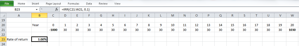
The spreadsheet calculates the internal rate of return (IRR) for a cash flow scenario. It spans columns B through W and rows 20 to 23.
-
Row 20 is labeled "Year" and contains values from 0 to 20 across columns C to W.
-
Row 21 lists cash flows for each year:
-
Year 0: -1000 (initial investment)
-
Years 1–19: 30 (constant annual returns)
-
Year 20: 1030 (final payment)
-
-
Row 23 shows the calculated "Rate of return" as 3.00% using the formula
=IRR(C21:W21, 0.1)displayed in the formula bar.
Old Bond Rate of Return Analysis
As explained before, buyers can sell their bonds in the market before their maturity dates.
Example 3-3
Assume person A buys the new bond that is explained in Example 3-2. After two years (in the end of the year), person A decides to sell the old bond to person B for 800 dollars. Calculate the rate of return of investment for person B.
Person B investment can be shown as:
| C = $800 | I=$30 | I=$30 | I=$30 | L = $1000 | |
|
|
|||||
| 0 | 1 | 2 | ... | 16 | |
We can write the equations for this investment as:
Present value of cost = present value of income
The trial and error technique or IRR function in Microsoft Excel gives that i = 4.82% per semi-annual period and a nominal rate of return 2*4.82 = 9.64%per year compounded semi-annually.
Note: the only thing different from previous the calculation is the time and investment cost.
Please watch the following video, Calculating return on a bond investment (7:53).
PRESENTER: In this video, I'm going to talk about bonds and how to calculate the return on a bond investment.
Bonds are financial tools that can help governments and corporations raise money for their investments. So a bond is a piece of document that simply says, I owe you. So there are three things that you need to know about the bond. The first one is the face value. When buyers buy bond, they pay the face value. The face value is the amount that is written on the bond at the time that it's issued. The second thing that you need to know about the bond is the maturity date, which actually means the expiration date. It is the date that buyers receive the face value of the bond. The third one is the interest that the issuer of the bond pays to the buyers of the bond, and it is called bond coupon and it will be paid as fixed amount. It can be annually or semiannually, every six months.
Some bonds allow the interest rate to be adjusted with the inflation rate. Some bonds can be converted to some common stock or other securities. The good thing about bond is the buyer of the bond doesn't need to wait until the maturity date and receive his or her money. Buyers of the bond can sell the bond at any time before the maturity date.
The price of a bond is dependent on the financial market and interest rate in the market can be higher or lower than the face value. If the interest rate in the market drops, then bond can be sold at the higher price than the face value. For example, if you buy a bond and in the market, the interest rate drops, you can sell your bond at the higher price than the face value because the bond has coupon, which means that you're going to receive fixed amounts of payments per year or per six months, and these are fixed. If the interest rate in the market drops, your bond has higher value in the market.
Usually, the issuer of the bond has to support or back the bond with some selected asset as collateral in case of bankruptcy. Bonds with higher level of risk pay higher interest rate. The interest rate has to be reported nominally, but the interest can be paid on the semiannual basis.
Let's work on this example. Let's assume you are going to buy a bond that has a face value of $1,000 with a maturity date of 10 years that pays you $30 every six months, and you want to calculate the return on this investment.
First, we draw the time line. We are going to have 20 time intervals because there are 10 years and each six months, we are going to receive $30. We are going to have $1,000 investment at the present time, and we are going to receive $30 every six months, which are going to be 20 payments of $30. And in the end, we are going to receive the $1,000 of the face value of the bond. And we are going to calculate the return on this project.
We write the equation. Present value of the cost should be equal to present value of income. Present value of the cost is the $1,000 that we pay for this investment at the present time, and we are going to receive 20 payments of $30. And in the end of the 10th year, which is going to be the 20th period, we are going to receive the face value of $1,000.
And then we have to solve this equation using the trial and error method or IRR function in Excel, which I'm going to explain in the next video. And we calculate the i as 3% per semiannual. And then we need to calculate the nominal rate of return, which equals 2 multiply 3%, which will be 6% per year, compounded semiannually. So this investment of buying a bond at the present time at the price of $1,000 with a maturity date of 10 years and a coupon of $30 being paid every six months, is going to have the return of 6% per year compounded semiannually. The 6% nominal rate of return that we calculated is also called yield to maturity or YTM.
Now, let's work on an other example-- old bond rate of return analysis. Let's assume person A buys a new bond that is explained in the previous example, and then this person wants to sell the bond after two years to the person B at $800. Let's calculate the rate of return in this investment for person B.
So again, the first thing that we have to do is we have to draw the time line. And here, because person A is selling the bond after two years to person B, we are going to have 16 periods of six months. Person B is buying the bond at the cost of $800, and person B is going to receive $30 every six months for 16 periods of six months. In the end of the eighth year or 16 six months, person B is going to receive the face value of $1,000. Please note that person B is buying the bond at $800 but is going to receive the face value of the bond at the end of the maturity date.
And we write the rate of return equation. Present value of cost equal to present value of income. Cost is going to be $800, and person B is going to receive 16 payments of $30 every six months and $1,000 in the end of the 16th period. And we calculate the rate of return for this investment using the trial and error technique or IRR function in Excel, which is going to be 4.82%. And again, this is per semiannual period. We need to report that as the nominal rates per year. So we have to multiply by 2. So we are going to get 9.64% per year compounded semiannually. This is the return on this investment.
Example 3-4
Assume interest rates in the financial market dropped, which causes the price of an old bond to increase. So, person A in Example 3-2 can sell the old bond after two years (in the end of the year) to person B for 1200 dollars. Calculate the rate of return of investment for person B.
Similar to Example 3-3, person B's investment can be shown as:
| C = $1200 | I=$30 | I=$30 | I=$30 | L = $1000 | |
|
|
|||||
| 0 | 1 | 2 | ... | 16 | |
Present value of cost = present value of income
And rate of return per semi-annual period will be i = 1.58% and the nominal rate of return is: 2*1.58 = 3.16%per year compounded semi-annually.
Example 3-5
Now assume this situation: Since the interest rate dropped in the financial market, the issuer organization can call the old bonds after 4 years (from now -- total maturity period of 6 years). This means that at that time, the issuer organization takes the bond and pays the face value. Please calculate the rate of return for person B’s investment if he buys the old bond at $1200.
Person B's investment can be shown as:
| C = $1200 | I=$30 | I=$30 | I=$30 | L = $1000 | |
|
|
|||||
| 0 | 1 | 2 | ... | 8 | |
Note that the old bond will be called in 4 years from now after person B buys it.
Present value of cost = present value of income
The rate of return for person B’s investment will be i = 0.45% per semi-annual period and the nominal rate of return: 0.9% per year compounded semi-annually.
Financial Cost of Capital and Opportunity Cost of Capital
As briefly explained in the first lesson, the financial cost of capital for a project (for a privately owned company) can be the average cost of financing current projects (or under consideration projects). The opportunity cost of capital or minimum rate of return (denoted as “i*”) reflects other opportunities that exist for the investment of capital now and in the future. The opportunity cost of capital for an investment is higher and more important than the financial cost of capital. An investor will invest in a project only if the rate of return is higher than opportunity cost capital (minimum rate of return).
Rate of return is a decision method to accept or reject a project and it is not a reliable method to rank several projects in terms of investment. Also, the rate of return for a current project is not necessarily applicable to future projects. For example, if an investment project has the rate of return of 5%, but another investment with similar (or lower) risk (such as interest paid by the bank to the money in your account or interest from buying Treasury Bond) has the rate of return of 6%, then the minimum rate of return and opportunity cost of capital will be 6%, and the project is not acceptable for investment.
If a company doesn’t have budget constraints, then it would keep investing in a new project until the rate of return on the next project is less than the cost of raising money. See Figure 3-3, below.
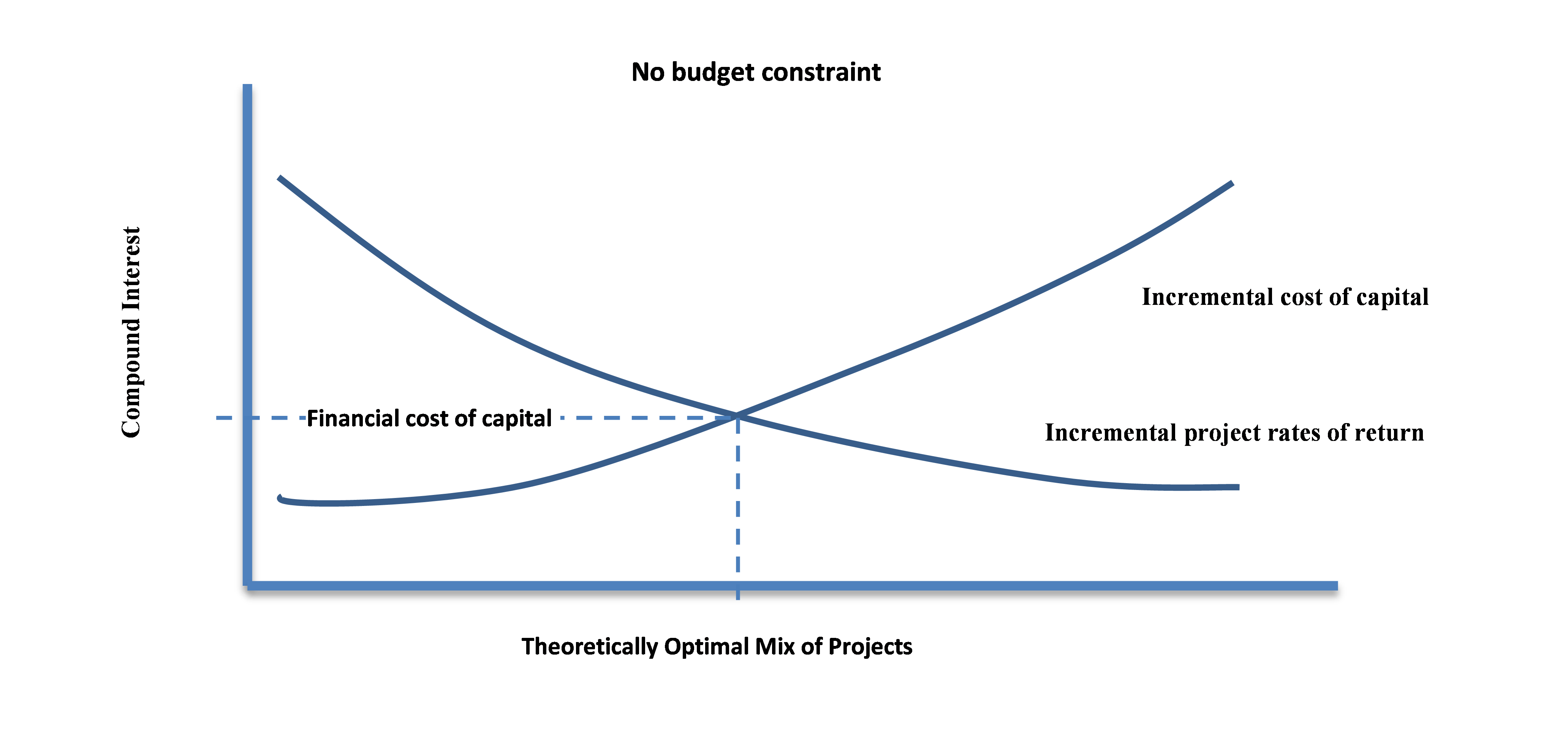
But this assumption is not usually realistic, and in the real world, there is always a budget constraint. As Figure 3-4 shows, budget constraint causes the cost of the capital curve to move upward and also to the left. In this case, the financial cost of capital needs to be adjusted to a minimum acceptable rate of return (MARR). The minimum acceptable rate of return reflects the project’s rate of return that is given up for the project under consideration.
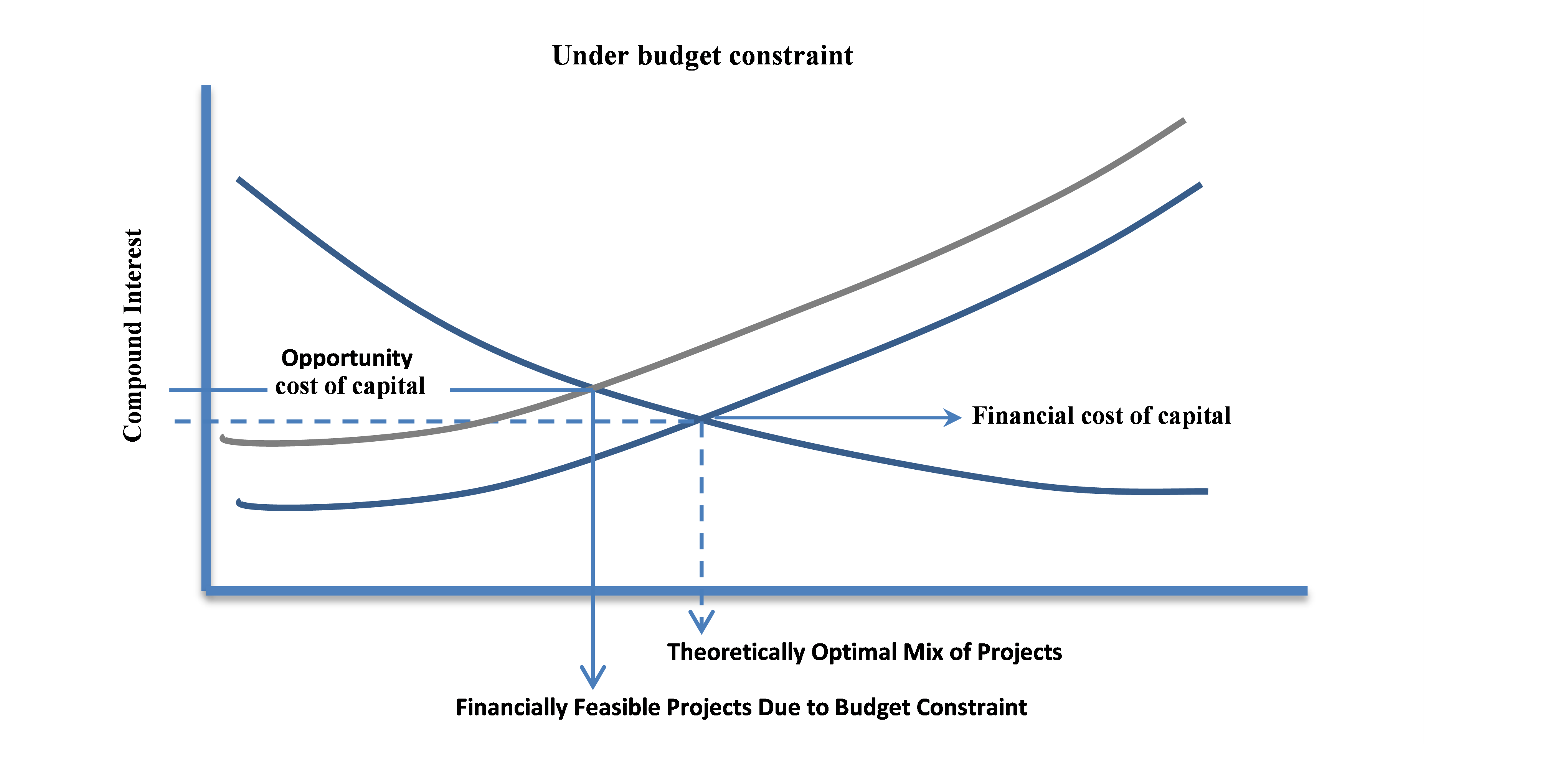
However, if the project that is under consideration is the only possible project or it is not comparable with other projects, or there is enough funding available for all other projects with a higher rate of returns, then the opportunity cost of capital can be equal to the financial cost of capital.
Net Present Value, Benefit Cost Ratio, and Present Value Ratio for project assessment
Net Present Value (NPV)
As explained in the first lesson, Net Present Value (NPV) is the cumulative present worth of positive and negative investment cash flow using a specified rate to handle the time value of money.
Or
Or
If the calculated NPV for a project is positive, then the project is satisfactory, and if NPV is negative then the project is not satisfactory.
The following video, NPV function in Excel, explains how NPV can be calculated using Microsoft Excel (8:04).
PRESENTER: In this video, I'm going to explain how to use NPV function in Excel to calculate the NPV of a cash flow. There are two main ways of calling NPV function in Excel. The first method is clicking in this little Fx here. When you click that, this window pops up, and then you can search the NPV function in this box.
You click Go. It finds the NPV function, or you can go to the Financial category here and you will find the NPV function. And then you click OK.
You can see three boxes here. The first one is asking you to enter the Rate. This rate is the interest rate that you're going to discount your cash flow when you calculate the NPV. You can write a number here, which is going to be 10%, or you can rate these from a cell, which I wrote 10% here. Then after, we can click this one or we can push Enter.
And then after, you can enter the cash flow. You can enter the cash flow one by one, in each of these values, or you can choose the cash flow as a series here. Then you click here. If you entered everything correctly, the NPV is going to be calculated and the function shows the NPV here. If something is wrong, you won't see a correct NPV here. Then I click OK. So as you can see, the NPV is calculated and shown.
The other way to call the NPV function is you just write equal sign, and then write NPV open parentheses, the first one, and then you can see did this thing pops up. In the first, you need to enter a rate. You can write a value here-- you can write 10%, or you can read it from this cell. And then you write a comma, and then you enter the values. You start from here, go all the way to the end of the cash flow. And you close the parentheses.
So one thing that you have to be very careful using the NPV function in Excel is NPV function in Excel always considers you are entering your cash flow from year 1. So if you have the cash flow that is happening at the present time, at time 0-- at year 0-- you have to enter that manually. NPV function in Excel does not consider any cash flow at time 0-- it doesn't understand a time 0. NPV assumes that you are entering everything from year 1.
So you can always double-check the result of this NPV function. If you calculate the present value of each of these payments, the summation of that discounted cash flow should be equal to this net present value. Let's quickly calculate that. Let's say we want to calculate the present value of these payments. The first one equals $50,000 divided by 1 plus interest rate. I put a dollar sign behind the column to fix this when I'm going to apply it to the other cells, and power, year.
So as you can see here, this is the present value of this $50,000 of investment. I apply that to the other cells. So the summation of this discounted cash flow, these present values, should be exactly the same as the NPV that we calculated using the NPV function in Excel, which you can see they are exactly the same.
So let's work on another example that has the cash flow at present time. So as you can see in this investment, we are going to have $60,000 of investment at present time, and also $50,000 of investment at year 1. This investment is going to yield the annual income of $24,000 a year, from year 2 to year 10. Let's see how we can calculate the NPV of this cash flow using the NPV function in Excel.
So as you can see here, because we are going to have a payment at present time, we need to enter that payment manually. So what we do is, we write the equal sign and then we add this payment, which is happening at the present time, or year 0. And then after, we use the NPV function for the rest of the cash flow. I write NPV-- I rate the interest rate from here. Then I select the cash flow, starting from the year 1 all the way to the year 10. I close the parentheses, and I press Enter. So this is the NPV, using the NPV function of this cash flow.
Let's double-check our result. Let's see if this is correct or not. So I'm going to calculate the present value of all these payments, and then the summation should be exactly same as this NPV-- using the NPV function. So present value equals this payment-- it is happening at the present time, so it doesn't need to be discounted. So it is equal same amount-- present value of this, $50,000, equals $50,000 divided by open parentheses 1 plus interest rate. I fix the column to make sure it doesn't change-- to make sure interest rates sale doesn't change when I'm going to apply to the other cells. I close the parentheses, and power, year. So this is the present value of this-- $50,000 happening at year 1.
So I apply this to the rest of cash flow, and the summation of this discounted cash flow should give me the exact same value as the NPV-- that I used the NPV function in Excel. As we can see, these are exactly the same.
So these are two ways of calculating NPV using Excel, and how we can double-check the other one.
In the video NPV and IRR in Excel 2010 [27] (8:59) you can find another useful video for calculating NPV using Excel NPV function. In this video, cash flow is formatted in the vertical direction (there is absolutely no difference between vertical and horizontal formatting, using spreadsheet).
In the following video, IRR function in Excel, I'm explaining how to calculate the Rate of Return for a given cash flow using Microsoft Excel IRR function (4:19).
PRESENTER: In this video, I'm going to explain how to calculate rate of return for a given cash flow using IRR function in Excel. There are two ways that we can call IRR function. First, we can click on this fx icon. This window pops up, and we can write IRR in this box, which is a search box. Go, it finds it. Or, we can choose the financial from this list and find the IRR.
When we choose IRR, this window opens up. And it has two boxes. The first box needs you to enter the cash flow. There's a very important point in calling Excel IRR function. That requires you to enter the cash flow, and it assumes your cash flow starts from year zero. So you should be very careful using IRR function in Excel. It assumes your cash flow starts from year zero or present time.
So I select the cash flow starting from year zero. And I click here or press Enter. So here, it already calculated the IRR. But sometimes, the IRR function cannot find a rate of return. So you need to give it an initial guess. If you don't have any assumption in your mind, just give it 10%. If still it doesn't calculate it, give it 20%, and so on. And you press OK. So as you can see here, the rate of return for this cash flow, starting from year zero, is 14.06%.
The other way to call the IRR function in Excel is just writing the IRR function. You write the equals sign, and then you write IRR. You can see Excel shows this here, shows the function here. You open the parentheses. You select the cash flow from starting from year zero all the way to the year 10. A comma, and the initial guess, which is going to be 10%. And the result.
So we can always double-check this result that we calculated rate of return using Excel IRR function. As you know, rate of return is a rate that makes NPV equal zero. So if I calculate the NPV for this rate, it should be exactly zero, or very close to zero. So let's see. Let's calculate the NPV for this rate.
So because we are going to have a payment at present time, I have to enter that payment manually. And then I have to calculate the NPV of the rest of the cash flows that start from year one using the NPV function.
NPV, open parentheses. Rates. I choose the rate. Comma, and then I select the cash flow that starts from year one. And I close parentheses. And you can see the NPV equals zero. So it shows that the rate of return that I calculated for this cash flow is correct.
Example 3-6:
Please calculate the NPV for the following cash flow, considering minimum discount rate of 10% and 15%.
| C=60,000 | C=50,000 | I=24,000 | I=24,000 | ... | I=24,000 |
|
|
|||||
| 0 | 1 | 2 | 3 | ... | 10 |
C: Cost, I:Income
If using spreadsheet, following method can be more convenient:
Figure 3-5 illustrates the calculation of the NPV function in Microsoft Excel. Please note that in order to use the NPV function in Microsoft Excel, all costs have to be entered with negative signs.
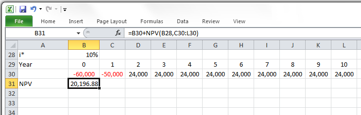
Benefit Cost Ratio
Benefit Cost Ratio (B/C ratio) or Cost Benefit Ratio is another criteria for project investment and is defined as present value of net positive cash flow divided by net negative cash flow at i*.
For the project assessment:
- If B/C >1 then project(s) is economically satisfactory
- If B/C =1 then project(s) the economic breakeven of the project is similar to other projects (with same discount rate or rate of return)
- If B/C <1 then project(s) is not economically satisfactory
Present Value Ratio
Present Value Ratio (PVR) can also be used for economic assessment of project(s) and it can be determined as net present value divided by net negative cash flow at i*.
- If PVR>0 then project(s) is economically satisfactory
- If PVR=0 then project(s) is in an economic breakeven with other projects (with same discount rate or rate of return)
- If PVR<0 then project(s) is not economically satisfactory
Example 3-7
Calculate the B/C ratio and PVR for the cash flow in Example 3-6.
Figure 3-6 illustrates the calculation of the B/C function in Microsoft Excel. Please note that you need to use the absolute value in the denominator or multiply the answer by -1.
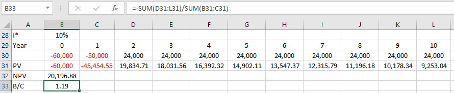
Figure 3-7 illustrates the calculation of the PVR function in Microsoft Excel. Please note that you need to use the absolute value in the denominator or multiply the answer by -1.
Summary and Final Tasks
Summary
In Lesson 3, we have learned that annual percentage rates (APR) represent an annualized expression of the cost of borrowing money, and how to calculate an APR based on a leader's cash flow. The salvage value is also introduced, which presents a positive cash flow for the project. Bonds are a very popular tool for corporations and governments to raise debt capital and we have learned the cash flows of a bond. The old bond rate or return with or without call privileges is also introduced. We also learned the concepts and effects of financial cost and opportunity cost of capital and in the last part we figured out how to evaluate a project(s) using Net Present Value, Benefit Cost Ratio, and Present Value Ratio.
Reminder - Complete all of the Lesson 3 tasks!
You have reached the end of Lesson 3! Double-check the to-do list on the Lesson 3 Overview page [28] to make sure you have completed all of the activities listed there before you begin Lesson 4.
Lesson 4: Mutually Exclusive Project Analysis
Introduction
Overview
Mutually exclusive projects: making an analysis of several alternatives from which only one can be selected, such as selecting the best way to provide service or to improve an existing operation or the best way to develop a new process, product, mining operation, or oil/gas reserve.
Non-mutually exclusive projects: analyzing several alternatives from which more than one can be selected depending on capital or budget restrictions, such as ranking research, development, and exploration projects to determine the best projects to fund with available dollars.
This lesson focuses on the analysis of mutually exclusive alternatives. Valid discounted cash flow criteria such as rate of return, net present value, and benefit-cost ratio are applied in very different ways in proper analysis of mutually exclusive and non-mutually exclusive alternative investments.
Learning Objectives
At the successful completion of this lesson, students should be able to:
- understand how to use rate of return and NPV analysis to evaluate mutually exclusive projects and non-mutually exclusive projects;
- understand how to conduct Incremental Analysis; and
- understand how variable minimum rate of return with time can affect the project.
What is due for Lesson 4?
This lesson will take us one week to complete. Please refer to the Course Syllabus for specific time frames and due dates. Specific directions for the assignment below can be found within this lesson.
| Reading | Read Chapter 4 of the textbook. |
|---|---|
| Assignment | Homework 4. |
Questions?
If you have any questions, please post them to our discussion forum, located under the Modules tab in Canvas. I will check that discussion forum daily to respond. While you are there, feel free to post your own responses if you, too, are able to help out a classmate.
Using Rate of Return, Net Value and Ratios for Mutually Exclusive Projects
Economic analysis of projects can be divided into two categories:
1) Mutually Exclusive
2) Non-Mutually Exclusive
Mutually Exclusive type analysis is where the investor faces different investment alternatives, but only one project can be chosen for investment. Selecting one project excludes other projects from investment.
Non-Mutually Exclusive assessments are where the investor faces different alternatives, but more than one project can be selected regarding capital or budget constraint.
Rate of Return Analysis for Mutually Exclusive Alternatives
Example 4-1: Assume an investor has two alternatives, project A and project B, and other opportunities exist to invest at 15% ROR. The total money that investor has is 400,000 dollars.
Project A: Includes investment of 40,000 dollars at present time which yields an income of 40,000 dollars for 5 years and the salvage value at the end of the fifth year is 40,000 dollars.
| C=$40,000 | I=$40,000 | I=$40,000 | I=$40,000 | I=$40,000 | I=$40,000 | L=$40,000 | |
| A) |
|
||||||
| 0 | 1 | 2 | 3 | 4 | 5 | ||
Project B: Includes investment of 400,000 dollars at the present time which yields the income of 200,000 dollars for 5 years and the salvage value at the end of the fifth year is 400,000 dollars.
| C=$$400,000 | I=$200,000 | I=$200,000 | I=$200,000 | I=$200,000 | I=$200,000 | L=$400,000 | |
| B) |
|
||||||
| 0 | 1 | 2 | 3 | 4 | 5 | ||
C: Cost, I:Income, L:Salvage
ROR analysis for project A:
With trial and error or using the IRR function in Excel, we can calculate . So project A is satisfactory.
ROR analysis for project B:
With trial and error or using the IRR function in Excel, we can calculate . So project B is also satisfactory.
Many people think because project A has a higher ROR, project A has to be selected over project B. But remember, we assumed 400,000 dollars is available for the investment, and the investor can only choose one of the projects. Project A takes just 10 percent of the money and gives 100% ROR, while project B takes the entire 400,000 dollars and gives 50% ROR. If the investor chooses project A and spends 40,000 dollars on this project, the rest of the money can only be invested with a 15% ROR. So, we need one more step that is called incremental analysis to be able to compare two projects and determine which project is better. The incremental analysis helps up to find a common base to compare two projects. To do so, incremental analysis breaks project B into two projects: one is similar to project A and the other is an incremental project.
Project B is equivalent to
Please note that the investing in Project B (requires $400,000) is equivalent to investing
Choosing project A with 100% ROR + investing the rest of money with 15%
Or
Choosing project B, which is equivalent to an investment in project A with 100% ROR+ investment in the incremental project (B-A)
The incremental analysis has to be done for the bigger project minus the smaller one as:
| C=$360,000 | I=$160,000 | I=$160,000 | I=$160,000 | I=$160,000 | I=$160,000 | L=$360,000 | ||
| B-A |
|
|||||||
| 0 | 1 | 2 | 3 | 4 | 5 | |||
This investment gives 44.4 % return.
So, incremental analysis shows that investment in project B is equivalent to investing in A (which gives 100% ROR) plus investing in project B-A (which gives 44%).
Thus, the second alternative, project B, is more desirable.
1) the rate of return on total individual project investment must be greater than or equal to the minimum rate of return, i*.
2) the ROR on incremental investment compared to the last satisfactory level of investment must be greater than or equal to the minimum ROR, i*.
The largest level of investment that satisfies both criteria is the economic choice.
Therefore, in mutually exclusive projects, a smaller ROR on a bigger investment often is economically better than a big ROR on a smaller investment. Therefore, it is often preferable to invest a large amount of money at a moderate rate of return rather than a small amount at a large return with the remainder having to be invested elsewhere at a specified minimum rate of return.
Please watch the following video (11:56): Mutually exclusive projects (Rate of return analysis).
PRESENTER: In this video, I'm going to explain how we can evaluate mutually exclusive projects. If you are given more than one investment project to evaluate, then you're facing two types of investments. It is either a non-mutually exclusive or mutually exclusive kind of problem. In a non-mutually exclusive assessment, you can choose more than one project. In this case, you will rank the project based on the parameter that you learn, such as the MPV rate of return and so on, and choose the projects from the best to worse.
But here, in this lesson, we are going to work on mutually exclusive evaluations. In this case, in mutually exclusive assessments, we have a budget constraint, so we can only choose one project. So we need to evaluate all projects and select the best project that is economically satisfactory.
Let's work on an example. Assume an investor has two alternatives, project A and project B, and other opportunities exist to invest at a 15% rate of return. And this 15% rate of return means we can make at least 15% on the $400,000 if we invest somewhere else. The $400,000 that isn't required for investment in project A or project B.
So it means each of these two projects, project A and project B are economically satisfactory only if each of them gives a return of higher than 15%. If they don't, they are not economically satisfactory, and we can invest in the other project with the 15% rate of return. So our minimum rate of return or minimum discount rate is 15%. This is the rate that we have to compare our individual assessment with.
So let's calculate the rate of return for these projects. So in order to evaluate and find-- in order to evaluate and find the best project, first, we have to evaluate each project individually. Then we compare the projects that are economically satisfactory and choose the best one. So let's calculate the rate of return for project A and project B.
First, we write the equation for the rate of return-- the present value of cost equals the present value of income plus salvage. And we calculate rate of return for project A as 53%, which is higher than 15% minimum rate of return. So it tells us that project A is economically satisfactory.
Now let's calculate the rate of return for project B. We write the equation. So we can see the rate of return for project B is 50%, which is higher than 15% of the minimum rate of return. So project B is also economically satisfactory. So because project A has a higher rate of return with the same amount of investment, we can conclude that project A has to be selected for the investment.
Now let's work on a slightly different example. Let's assume that the investor has $400,000 available for the investment. The investor has two alternatives, project A and project B, and other opportunities exist to invest at 15% rate of return. As you can see here, project A requires $40,000, but we have $400,000 money available for the investment. Again, first, we have to evaluate the projects individually, and then we compare the projects that are economically satisfactory and choose the best one.
So for project A, we write the equation to calculate the rate of return. And we calculate rate of return as 100%, which is higher than the 15% of minimum rate of return, so project A is economically satisfactory. Then we calculate the rate of return for project B. We write the equation, and we calculate the rate of return, which is 50%. 50% is higher than the minimum rate of return of 15%, so project B is also economically satisfactory.
So the results show that project A has a higher rate of return than project B. Let's see if project A is the best project for the investment or not. Using the rate of return for mutually exclusive projects can be confusing, and it doesn't necessarily give us the best economic choice. Remember, we had $400,000 available to investment, but project A is using only $40,000 of that $400,000. Project A is giving us a 100% return on $40,000, but project B is giving us a 50% return on the total $400,000.
This means if you invest in project A, then you will have an extra $360,000 that you can only invest in the other project with 15% return because project A requires only $40,000, but we have $400,000 available for the investment. So the rest of the money, that $360,000, can't be put in any other project other than the project that gives the minimum rate of return of 15%.
So there are two alternatives for the investment of $400,000. The first one is investing the $40,000 in project A with the rate of return of 100%, plus investing the rest of $360,000 with the rate of return of 15%. Or the second alternative is investing the entire $400,000 in project B with the rate of return of 50%. So we need to find a base to compare these two projects together.
In this case, we need incremental analysis, which breaks the project B into two projects. One is similar to project A and the other is an incremental project or B minus A. So project B is equivalent to project A-plus project B minus A because project A requires much less investment, and the rest of the money can only be invested in the minimum rate of return of 15%.
In order to evaluate the project B minus A, we need to deduct the project A cash inflow from the project B cash flow. So here, each year, each column, cash flow equals the project B minus project A. We write the rate of return equation for incremental cash flow-- the present value of cost equals the present value of income plus the present value of salvage. The present value of cost equals $360,000, which is the difference between project A and project B investment, and the $160,000, which is the difference between annual income for project A and Project B, and the $360,000 in year five, which is the difference between salvage values.
And we can use the Excel IRR function to calculate the rate of return. So incremental cash flow has the rate of return of 44.4%, and it is economically satisfactory. It means project B that has a rate of return of 50% is equivalent to project A with a 100% rate of return plus an incremental project with 44%.
So we have two alternatives. The first one is investing $40,000 at the rate of return of 100% plus investing $360,000 at the minimum rate of return of 15% or investing the entire $400,000 in project B, which is equivalent for investing in a project, similar to project A, with $40,000 of investment and the rate of return of 100% plus investing in the incremental project, which needs $360,000.
And the rate of return would be 44.4%. And we can conclude that project B is more desirable investment although project B has a lower rate of return. But because it uses the entire $400,000, it is a better project to invest.
When using the rate of return analysis for the evaluation of mutually exclusive projects, we need to keep two things in our mind. First, the rate of return for each individual project has to be higher than the minimum rate of return. And also, the rate of return on the incremental investment has to also be higher than the minimum rate of return.
And the largest level of investment that satisfies both criteria is the economic choice, So it is often more desirable to invest a large amount of money at a moderate rate of return rather than investing a small amount of money at a large rate of return because we need to invest the rest of the money at a minimum rate of return.
Net Present Value (NPV) Analysis of Mutually Exclusive Alternatives “A” and “B”
Considering a discount rate of 15% (minimum rate of return), the NPV for project A and B can be calculated as:
Since the NPV for project A and B is positive at the 15% discount rate (minimum rate of return on investment), then we can conclude that both projects are economically satisfactory. But NPV for project B is higher than A, which means B is a better choice to invest.
Incremental NPV Analysis
We can also calculate the incremental NPV as:
Note that incremental NPV is exactly equal to the difference between NPVA and NPVB:
The incremental at a 15% discount rate is positive, which means the incremental investment is economically satisfactory.
Remember the two decision alternatives that the investor faces:
1) Choosing project A + investing the rest of money with 15%
2) Choosing project B, which is equivalent to an investment in project A + investment in the incremental project (B-A)
The NPV for the first decision is:
1) NPVA + NPV (of investing the remainder of the available money somewhere else with a 15% rate of return)
If an investment return of 15%, then the NPV at a discount rate of 15% for that investment cash flow equals zero. So:
1)
The NPV for the second decision is:
2)
Therefore, it can be concluded that investment in project B is a better decision.
In summary, for net present value analysis of mutually exclusive choices, two requirements need to be tested: 1) the net value on total individual project investment must be positive, and 2) the incremental net value obtained in comparing the total investment net value to the net value of the last smaller satisfactory investment level must be positive. The largest level of investment that satisfies both criteria is the economic choice. Or simply, the project with the largest positive net present value is the best choice.
Note: You can use Microsoft Excel and the NPV function in order to calculate Net Present Value as explained in Example 3-6 in Lesson 3.
Please watch the following video (3:37): Mutually exclusive alternatives
PRESENTER: Another method to evaluate the mutually exclusive projects is the NPV analysis. So let's work on the same example using the NPV analysis.
Assume an investor has two alternatives, Project A and Project B, and the total money that the investor or has is $400,000, and the minimum rate of return is going to be 15%
First, we have to evaluate each project individually, and then we compared to projects that are economically satisfactory and choose the best one. So first, we have to calculate the NPV for Project A. We used the minimum rate of return of 15% as a discount rate for calculating the NPV. And because the NPV of Project A at a discount rate of 15% is positive, so we can conclude that Project A is economically satisfactory.
And then we calculate the NPV for Project B. NPV of Project B at a minimum rate of return of 15% is also positive, so Project B is also economically satisfactory.
So Project A and Project B, both have positive NPVs, so both of them are economically satisfactory. And because Project B has a higher NPV, we can conclude that Project B is a better project to invest in. This is a very good thing about NPV, that if a project has a higher NPV, we can directly conclude that that project is a better choice to invest.
We can also calculate the NPV for the incremental cash flow, which we can see here, it is positive, and we can conclude Project B is better than Project A.
But there is a good property for NPV operator is NPV of the incremental analysis, NPV of B minus A equals NPV of Project B minus NPV of Project A. So that's the reason that if we calculate the NPV of Project B higher than Project A, we can conclude that Project B is a better project to invest, because the difference shows us the increment, directly shows us the NPV of the incremental cash flow.
So again, we have two alternatives here, choosing Project A and investing the rest of the money at the 15% minimum rate of return, or choosing Project B, which is equivalent to investing in Project A plus investing in the incremental Project B minus A.
And because incremental NPV at a 15% discount rate is positive, it means that incremental investment is economically satisfactory, which means that a second alternative, or Project B, is a more desirable scenario.
Ratio Analysis of Mutually Exclusive Projects A and B
Present value ratio (PVR) also can be applied to analyze two mutually exclusive projects, A and B:
Positive PVR for project A and B indicates that both projects are economically satisfactory. But higher PVR for project A doesn’t necessarily mean project A is better than B for investment and PVR needs to be calculated for an incremental project as well.
Accepting the incremental investment indicated accepting project B over A, even though the total investment ratio on B is less than A. Just as with ROR analysis, the mutually exclusive alternative with bigger ROR, PVR is not necessarily a better mutually exclusive investment. Incremental analysis along with total individual project investment analysis is the key to a correct analysis of mutually exclusive choices.
Mutually Exclusive Projects with Unequal Life
If mutually exclusive projects that are being analyzed don’t have the same lifetimes (for example, one investment has a length of 8 years and the other alternative example has the length of 12 years), we have to be careful using the parameters that we have learned so far.
NPV analysis
We can continue the NPV analysis without any problem for mutually exclusive projects with different lifetimes. This is because NPV analysis considers a common point in time for all projects, which is the present time.
It is also important to know that for NPV analysis, different discount rates may cause different results and may change the ranking of the projects. Thus, the selected discount rate for such should be representative of the opportunity cost of capital for consistent economic decision-making.
ROR analysis
For ROR analysis (and other analysis, such as future value, that require a specific point on the timeline) of mutually exclusive projects with different lifetimes, we need to find a common lifetime and analyze the alternatives based on that. This common lifetime is usually the longest lifetime between alternatives.
For ROR analysis, treat all projects as having an equal life that is equal to the longest life project with net revenues and costs of zero in the later years of shorter life projects.
Example 4-2:
Consider the following two mutually exclusive projects:
Assume a minimum rate of return of 8%
Project A
| C=1000 | I=250 | I=250 | I=250 | I=250 | I=250 | I=250 | I=250 |
|
|
|||||||
| 0 | 1 | 2 | 3 | 4 | 5 | 6 | 7 |
Project B
| C=2000 | C=3000 | I=1000 | I=1000 | I=1000 | I=1000 | I=1000 | I=1000 | I=1000 | I=1000 | I=1000 |
|
|
||||||||||
| 0 | 1 | 2 | 3 | 4 | 5 | 6 | 7 | 8 | 9 | 10 |
First, we need to evaluate each project individually and see if both are economically satisfactory.
Project A evaluation:
For project A: ROR> i*=8%, NPV is positive, B/C is higher than 1, and PVR is positive. So, project A is economically satisfactory.
Project B evaluation:
For project B: ROR> i*=8%, NPV is positive, B/C is higher than 1, and PVR is positive. So, project B is also economically satisfactory.
Please note that project A has a lifetime of seven years, while project B’s lifetime is 10 years. In this case, we chose the project with the longest lifetime (here, project B) as the base case and put zero for the years that project A doesn’t have any payment. Then we deduct the cash flow of project A from the cash flow of project B as incremental cash flow:
| -1000 | -3250 | 750 | 750 | 750 | 750 | 750 | 750 | 1000 | 1000 | 1000 |
|
|
||||||||||
| 0 | 1 | 2 | 3 | 4 | 5 | 6 | 7 | 8 | 9 | 10 |
Since the incremental project (B-A) is economically satisfactory, we can conclude that project B is better than project A.
Note that
Example 4-3:
Consider this situation that a manager faces. There are three alternatives:
- investing in development plan A, as shown in the following cash flow;
- investing in development plan B, as shown in the following cash flow;
- selling the property for $150 in cash. Apply the ROR, NPV, and PVR analysis to find the best economic alternative assuming a minimum rate of return of 15%, and then repeat the assessment for a minimum rate of return of 20%.
| Year | 0 | 1 | 2 | 3 | 4 | 5 | 6 | 7 | 8 | 9 | 10 |
|---|---|---|---|---|---|---|---|---|---|---|---|
| A | -200 | -350 | 100 | 100 | 150 | 150 | 150 | 150 | 150 | -- | -- |
| B | -300 | -400 | 200 | 200 | 200 | 200 | 200 | 200 | 200 | 200 | 200 |
| Sell | 150 | -- | -- | -- | -- | -- | -- | -- | -- | -- | -- |
Figure 4-1: cash flow for three alternatives: 1) Development plan A, 2) Development plan B, 3) Sell the property
RORA = 13.2% ROR is less than minimum rate of return of 15%, so the project is not economically satisfactory
. NPV is negative, so the project is not economically satisfactory
. PVR is negative, so the project is not economically satisfactory.
RORB=21.65% ROR is higher than the minimum rate of return of 15%, so the project is economically satisfactory
. NPV is positive, so the project is economically satisfactory
. PVR is positive, so the project is economically satisfactory.
ROR, NPV, and PVR analysis indicate that development plan B is better than investing money at a minimum rate of return of 15%.
The NPV, ROR, and PVR for selling the property:
RORsell = +∞ higher than the minimum rate of return of 15%, so the project is economically satisfactory
NPVsell = +150 is positive, so the project is economically satisfactory
PVRsell = +∞ is positive, so the project is economically satisfactory
Since NPVB is higher than NPVsell, the above analyses show that development plan B is the best economic choice among the three alternatives.
In order to compare development plan B and selling the property, we can also apply the incremental analysis as:
| Year | 0 | 1 | 2 | 3 | 4 | 5 | 6 | 7 | 8 | 9 | 10 |
|---|---|---|---|---|---|---|---|---|---|---|---|
| B-sell | -450 | -400 | 200 | 200 | 200 | 200 | 200 | 200 | 200 | 200 | 200 |
which is greater than 15%, so project B is economically satisfactory.
is positive, so it is economically satisfactory.
0.04 is positive, so it is economically satisfactory.
As previously explained, the incremental analysis will always lead to selecting the alternative with the largest individual NPV. Therefore, development plan B is the best economic choice. However, note that project B does not have the highest ROR or PVR.
Assuming the minimum rate of return of 20%
It is negative, so the project is not economically satisfactory.
. NPV is positive, so the project is economically satisfactory
NPVsell= +150 is positive, so the project is economically satisfactory.
Therefore, at a minimum rate of return of 20%, selling the property is the best economic choice.
As calculations show, results are sensitive to discount rates (minimum rate of return)
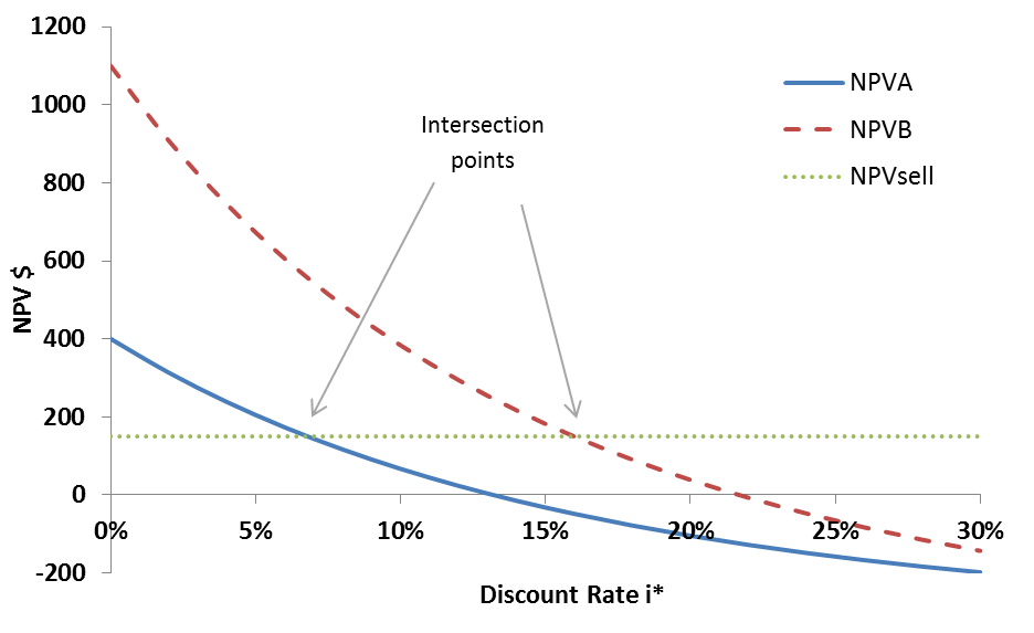
Mutually exclusive projects with different starting dates
Example 4-4:
Consider two alternatives: development plan B, and selling the property. But assume that development plan B will start in the second year. Which project is the best economic choice at a minimum rate of return of 15%?
Cash flow for these alternatives:
| Year | 0 | 1 | 2 | 3 | 4 | -- | 12 |
|---|---|---|---|---|---|---|---|
| B | -- | -- | -300 | -400 | 200 | 200 | 200 |
| Sell | 150 | -- | -- | -- | -- | -- | -- |
In this case, NPV indicates that selling the property is the best economic choice. NPV is positive, so it is economically satisfactory.
NPVsell=150 is positive, so it is economically satisfactory.
Incremental analysis can also be done as:
| Year | 0 | 1 | 2 | 3 | 4 | -- | 12 |
|---|---|---|---|---|---|---|---|
| B-sell | -150 | -- | -300 | -400 | 200 | 200 | 200 |
RORB-sell = 14.57% which is lower than 15% minimum rate of return
which is negative, so it is not economically satisfactory.
Thus, choosing development plan B overselling the property is not economically acceptable.
Changing the Minimum Rate of Return with Time
So far, we have assumed that minimum rate of return is fixed over the life of the project. But there are situations where other opportunities for investment (that determine the minimum rate of return) can make different rate of returns in different time. Thus, minimum rate of return can change over time. For example, other opportunities for investment of capital can give i*=12% now; and three years from now, we might expect a project that has a return on investment of i*=15%.
For analyses with minimum rate of return that change with time, NPV and PVR are recommended as the best methods. ROR is not a reliable approach for such analyses.
Example 4-5:
Cash flows for two mutually exclusive investment projects A and B are given as:
| C=$40 | I=$20 | I=$20 | I=$20 | I=$20 | I=$20 | L=$40 | |
| A) |
|
||||||
| 0 | 1 | 2 | 3 | ... | 10 | ||
| C=$50 | I=$25 | I=$25 | I=$25 | I=$25 | I=$25 | L=$50 | |
| B) |
|
||||||
| 0 | 1 | 2 | 3 | ... | 10 | ||
C: Cost, I:Income, L:Salvage
Analyze these alternatives, assuming the minimum rate of return for the first and second years is 25% and for third to tenth year it is 15%.
Results indicate that project B is a better economic investment.
Note:
After year 2, minimum rate of return changes from 25% to 15%. In order to calculate the NPV of the cash flow, we have to separate the payments that happened at and before year 2 from payments that occurred after year 2.
Payments at year 2 and before that are not going to be affected by the change:
PV of payments from year 0 to year 2:
Project A: Present value of year 0 to year 2 payments
Project B: Present value of year 0 to year 2 payments
But payments after year 2 will be affected by the change.
To calculate the NPV of those payments and apply the change in i, first, we need to discount all the payments occurred after year 2 to this year (we set the year 2 as the base year) by i* = 15% and we calculate value of all payments at year 2:
Project A: Value of year 3 to year 10 payments at year 2
Project B: Value of year 3 to year 10 payments at year 2
Second, we discount the year 2 values for 2 years by i* = 25%to get the present value (value at year 0) of the payments:
Project A: Present Value of year 3 to year 10 payments
Project B: Present Value of year 3 to year 10 payments
In the end, we add all the values together:
Another Method:
You can also treat each payment separately. This method is especially helpful when payments are not equal or when you are using spreadsheet to calculate the NPV.
We separate the payments that happened at and before year 2 from payments after year 2. Payments at and before year 2 will be discounted just by 25%:
PV of payments from year 0 to year 2:
Project A: PV year 0 to year 2
Project B: PV year 0 to year 2
For payments after year 2, first we calculate their value at year 2:
Project A: Value of year 3 to year 10 payments at year 2
Project B: Value of year 3 to year 10 payments at year 2
Second step, we discount the year 2 values for 2 years by i* = 25% to get the present value (value at year 0) of the payments:
Project A: Present Value of year 3 to year 10 payments
Project B: Present Value of year 3 to year 10 payments
In the end we add all the values together:
Microsoft Excel or Spreadsheet
If you are using Microsoft Excel or another spreadsheet to calculate the Net Present Value for the cash flow that has different discount rates over the life of project, be careful! You can not use the NPV function. However, you can calculate the Net Present Value by making a summation over calculated discounted cash flow. Figure 4-3 displays how Net Present Value for Project A cash flow with a changing minimum rate of return can be calculated. Note the formula in the cell D3 to D12.
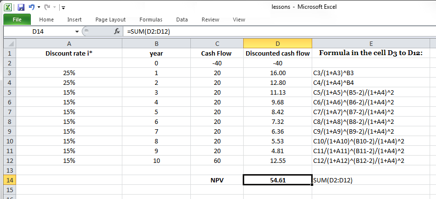
PRESENTER: So far, we assume the minimum rate of return in our analysis is fixed over the lifetime of the project. And it's not changing over time. But there are situations that we might have other opportunities for investment later on in the following years. So our minimum rate of return might change.
And it means that the discount rate, the minimum discount rate that we are using in our analysis will change too. In this video, I'm going to explain how we can evaluate the mutually exclusive projects or, in general, any other project if the minimum rate of return, if the discount rate changes over the lifetime of a project. So if the minimum rate of return changes with the time, the NPV and PVR present value ratio are recommended as the best methods. And rate of return is not a reliable approach for the project evaluation.
Let's work on this example. We have the cash flow for Project A and Project B that are mutually exclusive. And we assume the minimum rate of return for the first and second year is 25%. And the minimum rate of return changes to 15% from year 3 to year 10. So the first thing that we have to do is to separate the payments before the change and after the change.
So here, minimum rate of return changes after year 2. So I draw this red vertical line here to separate the payments before this year and payments that are after year 2. Return of present value of 40. Present value of these 20 payments at year 1 and 2. So present value of 40 is $40. And it is negative because it's a cost, it's an investment, and it's happening at present time. So there is no discounting needed here.
But two payments. We have two payments of $20 at year 1 and year 2. We discount them on 25%. And there are two of them. And then we need to calculate the present value of payments that are happening after year 2.
These payments are going to be affected by the change in the minimum rate of return. So first, we need to calculate the present value of these payments at 15% rate of return through the year 2 and then after discount at present value for 2 years with 25% of discount rate. So here, we have 8 payments of $20.
So we discount them 20 year 2 by the 15%. And then after, we discount that by 25% for 2 years. That is going to give us the present value here. And for the salvage value, it's the same. We discount the salvage value for 8 years at 15% and then we discount that after 2 years by 25%.
So we use this method to calculate the present value, net present value, NPV, for two mutually exclusive projects. And as we can see here, Project B has higher net present value. So I'm going to show you how we can calculate this in Excel using the other method, calculating the present value of each payment, and then add them back together. So I have the cash flow of Project A here, cash flow of Project B, and I wrote the minimum rate of return here for each year.
So as we can see here, we have 25% for year 1 and 2. And we have 15% from year 3 to year 10. So cash flow of Project A, cash flow of Project B. And for the last year, I added the salvage to the annual payment of the last year. So Project A, I'm going to calculate the present value of each payment in this cell.
So present value of these $40 of investment is going to be the same as $40. It doesn't need to be discounted because it is happening at the year 0. So present value of the $20. So I write equal sign at $20 divided by 1 plus interest rate, power, the year. So this is not going to be affected by change in the minimum rate of return.
So these 2 years are the same, so I just apply this equation to for the year 2. But for the year 3, how do we calculate the present value of this $20 that is happening at year 3? So it is going to be affected by two interest rates. 20 divided by open parentheses, 1 plus 15% power. So this needs to be discounted for 1 year because minimum rate of return changes at year 2. And this payment is 1 year away from year 2.
So I write year 1. And again, I have to divide that. I have to discount that by 2 years because this is going to give me the present value of this $20 here. And then I need to discount that at the rate of 25% for 2 more years. So 1 plus 25% power 2. And this is the same for the rest. So in order to apply these to the other cells, I will just write for this.
So read the year from here and minus 2, which is the year that the minimum rate of return changes. And I apply this to the other cash flow. And the same for Project B. Investment at present time as the same for year 1. It equals 1 plus 25% power the year.
For year 1 and year 2, there are similar. For year 3, this is 25 divided by open parentheses 1 plus 15% interest rate power year minus 2. And again, this divided by 1 plus 25% power 2.
And I apply this to the end. So these two should give me the present value. And I calculate the NPV for Project A, NPV for Project B. NPV for Project A equals the summation of all these present values. And the same for B.
Summary and Final Tasks
Summary
1. Mutually Exclusive Alternative Analysis
The Rate of Return or Growth Rate of Return: With either regular ROR or Growth ROR analysis of mutually exclusive alternatives, you must evaluate both total investment ROR and incremental investment ROR, selecting the largest investment for which both are satisfactory. Use a common evaluation life for Growth ROR analysis of unequal life alternatives, normally the life of the longest life alternative assuming net revenues and costs are zero in the later years of shorter life alternatives.
Net Value Analysis: With NPV analysis, you want the mutually exclusive alternative with the largest net value – because this is the alternative with the largest investment that has both a positive total investment net value and a positive incremental net value compared to the last satisfactory smaller investment.
2. Non-Mutually Exclusive Alternatives
The Rate of Return or Growth Rate of Return: Regular ROR analysis cannot be used to consistently rank non-mutually-exclusive alternatives. Use Growth ROR, and rank the alternatives in the order of decreasing Growth ROR. This will maximize profit from available investment capital. Use a common evaluation life for Growth ROR analysis for unequal life alternatives, normally the life of the longest alternative.
Net Value Analysis: With NPV analysis of non-mutually exclusive projects, select the group of projects that will maximize cumulative net value for the dollars available to invest. This does not necessarily involve selecting the project with the largest net value on individual project investment.
Reminder - Complete all of the Lesson 4 tasks!
You have reached the end of Lesson 4! Double-check the to-do list on the Lesson 4 Overview page [29] to make sure you have completed all of the activities listed there before you begin Lesson 5.
Lesson 5: Escalated, Nominal Price and Real Price
Inflation and Escalation in Economics
Inflation
Inflation is an economic term that indicates the increase in price of goods and services over time and can be more precisely defined as “a persistent rise in the prices associated with a basket of goods and services that is not offset by increased productivity.” Inflation causes purchasing power to reduce (more information can be found at Inflation (Investopedia) [30] and at Inflation (Wikipedia [31]). Inflation affects almost everything in the financial market and it is measured and reported by various indexes. The most common index for determining the inflation rate is called the Consumer Price Index [32] or CPI. You can read more about the CPI at the Wikipedia page for Consumer Price Index [33]. Monthly CPI reports are published at the U.S. Bureau of Labor Statistics website [34].
Escalation
"Escalation refers to a persistent rise in the price of specific commodities, goods, or services due to a combination of inflation, supply/demand, and other effects such as environmental and engineering changes." Factors that affect the escalation include:
- Inflation
- Supply/demand
- Technological Changes
- Environmental Effects
- Political Effects
- Miscellaneous Effects
As defined above, inflation refers to the increased price of a basket of goods and services, while escalation refers to an increase in price of a specified good or service. Inflation is one of the factors that cause escalation. The Alaskan pipeline is a good example that can help with understanding the difference between inflation and escalation. This pipeline was estimated to cost about 900 million dollars in 1969, while the final estimate in 1977 came to about 8 billion dollars for the project, which is around 900% higher than the initial estimation. You should note that just a portion of this increase was due to the inflation rate and that other factors such as supply/demand effects on labor and materials, and environmental and technology changes also contributed to the substantial increase in costs.
There are two techniques used to take into account the effect of inflation and escalation in economic analysis. Both methods should lead into the same results:
1. Escalated dollar analysis
"Escalated dollar values refer to actual dollars of revenue or cost that will be realized or incurred at a specific future point in time."
2. Constant dollar analysis
"Constant dollar values refer to hypothetical constant purchasing power dollars obtained by discounting escalated dollar values at the inflation rate to some arbitrary point in time, which often is the time that corresponds to the beginning of a project. Constant dollars are referred to as real dollars or deflated dollars in many places in the literature."
Escalated dollar analysis considers different purchasing power for different points in time, while constant dollar analysis aims to set a same base and a constant purchasing power for all points in time. Constant dollar analysis requires more calculation and the chance of making mistakes increases, while escalated dollar analysis has more reliable results. Escalated dollar and constant dollar analysis are two different methods and their results shouldn’t be compared. A common mistake in applying the results of constant dollar analysis is to compare the calculated constant dollar ROR with other escalated dollars investment opportunities such as bank interest rate and so on. Therefore, constant dollar ROR for alternative investment opportunities (constant dollar minimum rate of return) should be the base for comparing and evaluating constant dollar analysis for an investment project.
Usually reported cost, revenue, and incomes occurring in different points of time are reported at today’s dollar. Escalated dollar approach applies an assumed escalation rate to predict and increase the sums over time. To do so, similar to compounding technique, a single payment compound amount factor (F/Pi,n) has to be multiplied by the amount, and escalation rate has to be substituted for i.
For example, consider an investment with the following cashflow:
| C0=$10,000 | C1=$10,000 | I2=$15,000 | I3=$15,000 |
|
|
|||
| 0 | 1 | 2 | 3 |
C: Capital Cost, I: Income
Assuming an escalation rate of 12%, escalated dollar cashflow is:
| C0=$10,000 | C1=$10,000*(F/P12%,1) =$11,200 |
I2=$15,000*(F/P12%,2) =$18,816 |
I3=$15,000*(F/P12%,3) =$21,074 |
|
|
|||
| 0 | 1 | 2 | 3 |
Please watch the following video (6:25) Inflation, escalation, and escalated dollar analysis.
PRESENTER: In this video, I will explain how to consider inflation and escalation in the economic evaluation of investing project. Inflation is the economic term that indicates the average increase in price over the time. It is usually calculated for a basket of goods or services.
The most common index for determining the inflation rate is called CPI, or Consumer Price Index, and it is published by US Bureau of Labor Statistics. For example, the percentage change in CPI in a year compared to previous year indicates the inflation rate for that year.
Inflation causes purchasing power to reduce. For example, if you had $100 last year and the inflation rate is 5%, it means you won't be able to buy the same thing that you could buy last year. You can buy less.
Escalation is also referred to the price increase, but it is defined for only one good or service. Inflation is reported for basket of goods or service, and it is kind of a general average for the entire economy. But escalation is only for one good or service. So if price of a good or service increases, it can be because of inflation, supply and demand change, technological change, environmental effects, or political effects.
Two techniques are used to take into account the effect of inflation and escalation in economic analysis. Both of them should give you the same result. These two are called escalated dollar and constant dollar.
In escalated dollar analysis, you let your values, payments, income, costs, to be increased according to an escalation rate. In the constant dollar analysis, you will remove the effect of inflation from the increase value, from the escalated cash flow, meaning that you want to consider a hypothetical constant purchasing power.
One thing that you should keep in mind is you can do the constant dollar analysis only when you consider the escalation, only after escalated dollar analysis is done. Escalated and constant dollar analysis are two different methods, and the result shouldn't be compared.
Usually the reported cost, revenue and incomes are happening at different time, and they're reported at today's dollar. Escalated dollar analysis lets you apply the escalation rates to these payments. You assume an escalation rate, and you will predict the increase of each payment over the time.
In order to calculate the escalated dollar cash flow, you will compound each year's payment by the escalation rate, and you will have the escalation cash flow. If you do that for every single year for all the payments, you will have escalated cash flow in the end.
So let's work on this example. Assume this cash flow. We are going to have the investments of $10,000 at the present time and in year 1, and we are going to have the income of $15,000 at year 2 and year 3.
So let's calculate the escalated cash flow, the escalated dollar cash flow, for this investment, considering the escalation rate of 12%. As I explained in previous slides, in order to calculate the escalated dollar cash flow, we need to compound each payment by the escalation rate of 12%. So we need to multiply each year's cash flow by the factor F over P and the escalation rate.
So as you can see here, the present time payment is not going to be affected by the escalation. The first payment, which was at year 1, is going to be multiplied by the factor F over P, 12% of escalation rate, and 1 year of compounding. And the same for the other payments. So the $15,000 of income in the year 2 is going to be compounded for 2 years and 12% of escalation rate, and last year, year 3, it has to be compounded for 3 years by 12% of escalation rate.
And we calculate the result for each year. So the result is going to show us the escalated dollar cash flow considering the escalation rate of 12% for the original cash flow.
In order to calculate escalated dollar cash flow, we need to consider an escalation rate. Many, many investors use the anticipated inflation rate as the escalation rate to calculate the escalated dollar cash flow. But there are commodities, such as construction equipment, steel, concrete, labor, and energy, that may not follow this approximation. We can also have the negative escalation rate in case we are going to anticipate any decrease in costs, revenue, or income.
Escalation rate includes the inflation rate, and constant dollar approach applies a constant purchasing power by removing the effect of inflation rate from escalated dollars. Inflation effect can be removed, similar to discounting technique, by multiplying the single payment present worth factor (P/Fi,n) by escalated dollars and applying inflation rate as i. Many investors choose to utilize the anticipated inflation over future years as an approximation for escalation. Commodity prices, the price for construction equipment, steel, concrete, labor, and energy, may not move in direct correlation with the rate of inflation. Note that negative escalation rate can also be applied, if decrease in costs, revenue, or income is anticipated.
For example, considering inflation rate of 6% for above escalated dollar cashflow, constant dollar cashflow can be calculated as:
| C0=$10,000 | C1=$11,200*(P/F6%,1) =$10,566.04 |
I2=$18,816*(P/F6%,2) =$16,746.17 |
I3=$21,074*(P/F6%,3) =$17,694.07 |
|
|
|||
| 0 | 1 | 2 | 3 |
Please watch the following video (4:11): Constant dollar analysis.
PRESENTER: In this video, I'm going to explain how to apply the constant dollar analysis on an escalated cash flow for a project evaluation. As I explained in previous video, inflation is an indication that shows the increase in the price of a basket of goods or services over the time. But escalation is an indication of a price increase for one good or service.
I explain that we can calculate the escalated cash flow, escalated dollar cash flow, by the compounding payment at each year by the escalation rate. In the constant dollar technique, we will try to remove the effect of inflation in considering constant purchasing power. Because the escalation rate includes inflation, and we want to remove this effect and consider the hypothetical constant purchasing power. We can remove the effect of inflation from the escalated dollar cash flow by discounting payment at each year, considering that the inflation rate.
Let me explain how to calculate the constant dollar cash flow in an example. So in previous example in a previous video, we apply the escalation rate of 12% for the given cash flow that we had. So in order to calculate the escalated dollar cash flow, we compound each year's payment, each payment, by 12% escalation rate, and we calculated the escalated dollar cash flow, which is the escalated dollar cash flow, as you can see here.
So now we want to remove the effect of inflation rates and calculate the constant dollar cash flow. Please note that constant dollar cash flow can be calculated only after you already calculated the escalated dollar cash flow. You already consider it an escalation for your payments. Now, you want to remove the effect of inflation, and you want to consider the constant purchasing power and calculate, which means calculating constant dollar cash flow.
So in order to calculate the constant dollar cash flow, we need to discount each year payment, each year cash flow, by the inflation rate. So present time payment is not going to be affected by any inflation or escalation. Escalated payments at year one, $11,200. So we want to calculate the constant dollar for this payment. We multiply it by-- we discount it by one year, and 6%, and so on for the other payments.
Year three, we discounted for three discounting period and 6% of inflation rate. And the result. So the escalated dollar of $11,200 in the year 1 equals the constant dollar of $10,566. It means considering the inflation rate, the escalated dollar of $11,200 in the year one has the same purchasing power as $10,566 at the present time.
Last but not least, gold has been considered a good hedge against the long-term impact of inflation. Back in 1990, the gold price was $420 per ounce. In 2000, price fell to about $275 per ounce. That means an annual price decline of 4.1% per year over 10 years. During the same period, US inflation (as measured by CPI) averaged approximately 3% per year. If gold price would have increased in value at the rate of inflation, the value in 2000 would have been:
Instead, the actual price dropped to $275 per ounce and the corresponding constant dollar equivalent price of gold dropped to
In 2008, the gold trading price was $925 per ounce, an investment in an ounce of gold in 1990 would have produced an average annual rate of return of
After adjusting for an assumed 3% per year inflation, the real return on your investment would be closer to 1.4% per year. The calculations related to this type of constant dollar measure of economic performance will be developed in the Example 5-1 on the next page.
Practice Example:
Currently (May 2020) gold is trading at around $1,700 per ounce. How much would be the average annual rate of return of an investment in one ounce of gold in 1990? How much would be the rate of return, adjusted for inflation, assuming 3% per year of inflation in average?
Answer: 4.77% and 1.7% (approx.)
Italicized sections are from Stermole, F.J., Stermole, J.M. (2014) Economic Evaluation and Investment Decision Methods, 14th edition. Lakewood, Colorado: Investment Evaluations Co.
Escalated and Constant Dollar Cash Flow
The following examples can help you better understand escalated and constant dollar analysis.
Example 5-1:
Calculate the ROR for the investment that includes 1,000 and 1,200 dollar costs at the present time and at the end of the first year, which yields 800, 1,200, and 1,600 dollars of income at the end of the second, third, and fourth years. There is no salvage value.
Cash flow for this investment can be shown as:
| C0=$1,000 | C1=$1,200 | I2=$800 | I3=$1,200 | I4=$1,600 |
|
|
||||
| 0 | 1 | 2 | 3 | 4 |
By the trial and error method or with the IRR formula in Microsoft Excel, ROR for this project is calculated as: i=20.5%.
Figure 5-1 shows how this problem can be formulated in Microsoft Excel.
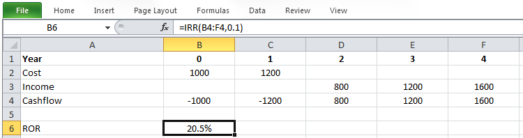
Escalated Dollar Analysis
Example 5-2:
Now assume for the above investment, costs and incomes will be escalated with the rate of 18% and 12% per year. Calculate the escalated dollar ROR for this investment.
For the escalated method, we need to utilize single payment compound amount factors (F/Pi,n) to convert (compound) the today’s dollar value to escalated dollar regarding the escalation rate:
| C0=$1,000 | C1=$1,200*(F/P18%,1) =1,416 |
I2=$800*(F/P12%,2) =1,003.52 |
I3=$1,200*(F/P12%,3) =1,685.91 |
I4=$1,600*(F/P12%,4) =2,517.63 |
|
|
||||
| 0 | 1 | 2 | 3 | 4 |
Note that escalation has no effect on the cost in the present time (1,000 dollars) because it assumes that all the amounts happen at the end of the year.
The rest of the solution for determining ROR is similar to before:
And ROR for this project is calculated as: i=33.6%. Figure 5-2 displays the way this problem can be formulated in Microsoft Excel..
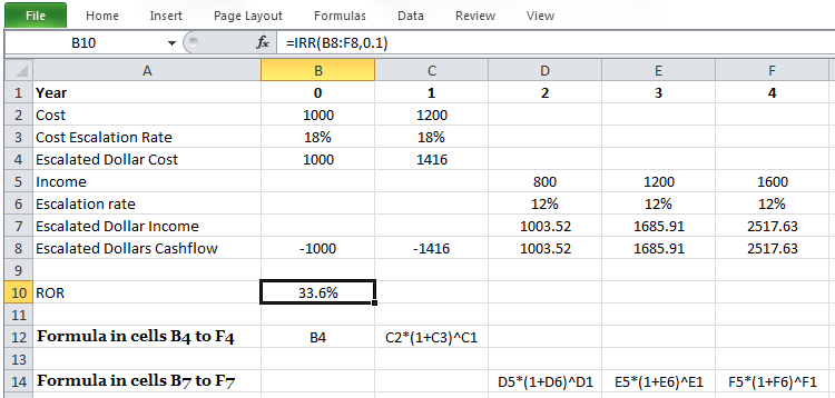
Constant Dollar Analysis
Example 5-3:
Now, determine the constant dollar ROR for the investment explained in Example 5-2 assuming an annual inflation rate of 15%.
In order to remove the effect of the inflation rate from our calculations, we need to discount the escalated dollars from previous analysis at the rate of inflation to express all dollar values in terms of time zero purchasing power. It can be done using the single payment present worth factor (P/Fi,n) with the assumed inflation rate.
| C0=$1,000 | C1=$1,416*(P/F15%,1) =1,231.30 |
I2=$1,003.52*(P/F15%,2) = 758.81 |
I3=$1,685.91*(P/F15%,3) = 1,108.52 |
I4=$2,517.63*(P/F15%,4) = 1,439.46 |
|
|
||||
| 0 | 1 | 2 | 3 | 4 |
Here, $1,231.30 at year 0 would purchase the goods and service that $1,416 would purchase at year 1, if inflation is 15% per year. $758.81 at year 0 would purchase the goods and services that $1,003.52 would purchase at year 2 if inflation is 15% per year and so on. The rest of the calculations are similar to before:
Where i' equals constant dollar ROR. And i'= 16.2% is calculated as ROR for constant dollar.
The following figure displays how constant dollar analysis can be formulated in Microsoft Excel.
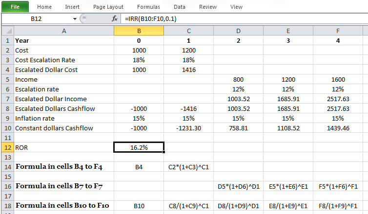
Please watch the following video (6:28): Escalated and constant dollar rate of return analysis.
PRESENTER: Let's work on an example to calculate the rate of return for escalated dollar cash flow and also constant dollar cash flow. This cash flow is given for an investment. So let's calculate the rate of return. In order to calculate the rate of return, we'd write the equation,the present value of costs equals the present value of income plus the present value of salvage. We don't have salvage value here. So the present value of costs equals the present value of income. We have two costs here-- $1,000 at present time and $1,200 at year one. And we're going to have three incomes of $800, $1,200, and $1,600 in a year two, three, and four.
So we write the equation and solve it for I and calculate the rate of return as 20.5%. Now let's consider an escalation rate of 18% for costs and escalation rate of 12% for income. Let's calculate the escalated dollar cash flow and then we will calculate the rate of return for the escalated dollar cash flow. In order to calculate the escalated dollar cash flow, we need to compound each payment by the escalation rate and considering the compound periods.
The payment at year 0 is not going to be affected by the escalation. So it stays unchanged. The cost of $1,200 at year 1 will be compounded with an 18% escalation rate because this is a cost and the compounding period will be 1. The income of $800 at year 2 will be escalated with 12% because this is an income and the compounding period will be two years and so on-- the income of $1,200 at year three, 12% escalation rate and three years compounding period and $1,600 income, 12% escalation rate and 4 compounding period-- and the result.
So we are going to have escalated cash flow at this cash flow that we can see here. And we want to calculate the rate of return for this escalated dollar cash flow. Again, we write the equation, the present value of cost equals the present value of all income. We have 2 costs here-- $1,000 and $1,416, which are escalating dollar cash flow. So if we write the equation, the present value of costs equals the present value of income, we have three incomes here-- the income at year 2, income at year 3, and income at year 4.
And we solve this equation for I. And we calculate that escalated dollar rate of return as 33.6%. So we calculated our escalated cash flow as the cash that you can see here. Now let's consider the inflation rate of 15%, and let's calculate the constant dollar cash flow and then calculate the rate of return for the constant dollar cash flow.
In order to remove the effect of the inflation rate from our calculations, from our escalated dollar cash flow, we need to discount each payment in the escalated cash flow by the inflation rate and considering the discounting period. So we need to multiply each payment and the escalated cash flow by the single payment present worth factor or factor p over f, considering the inflation rate and the discounting period to calculate the constant dollar cash flow. So as you can see here, we discount each payment by the inflation rate, which was 15%, and the discounting period.
You know that the present time is not going to be affected by the inflation rate. So we start from year 1, the escalated dollar cash flow. We multiply it by the single payment prison worth factor. This 15% is the inflation rate. And 1 is the discounting period. For year 2, the same inflation rates. The discounted period is going to be 2, and so on for year 3 and year 4.
And we calculate the result, which shows the constant dollar cash flow. So it means, for example, $1,231 at year 0 would have the same purchasing power as $1,416 in year 1. And let's calculate the rate of return for these constant dollar cash flow. Again, the equation is the present value of cost equals the present value of income. We have two constant-dollar costs and three incomes. So if we write the equation and we solve it for I and we calculate that the constant dollar rate of return as 16.2%. So we show it with I prime. And it is the constant dollar rate of return.
After calculating the ROR for the project, in order to complete the assessment and make the proper decision, it is necessary to compare it with the minimum rate of return (that is determined by other investment opportunities) to see if the project is economically satisfactory. To do so, you should be very careful using the proper minimum rate of return that is reported in escalated or constant dollars. For example, if other investment opportunities give 25% ROR on escalated dollars (it means the minimum rate of return on escalated dollars is 25%), we can conclude that this project with ROR of 33.6% is economically satisfactory. But the minimum rate of return of 25% on escalated dollars can’t be compared with the calculated 16.2% constant dollar.
As you can see in Example 5-2 and 5-3 for ROR calculations, P/Fi,n and P/Ff,n * P/Fi’,nsub> are similar:
i: escalated dollar ROR
i': constant dollar ROR
f: inflation rate
This mathematical proof is known as the “Fisher Rule [35].” This equation is a simpler way for calculating constant dollar ROR given the inflation rate and escalated dollar ROR. For example, i= 33.6% was calculated in Example 5-2 as ROR for escalated dollar analysis. In Example 5-3, ROR for a constant dollar is asked for the inflation rate of 15%. According to Equation 5-1, equals constant dollar ROR can be determined:
Which is equal to the Example 5-3 results.
Equation 5-1 can also be utilized to determine the minimum rate of return for constant dollars knowing the inflation rate and minimum rate of return for escalated dollars. In this case, i should be replaced with i* and i' with i'*:
i*: escalated dollar minimum rate of return
i'*: constant dollar minimum rate of return
f: inflation rate
For example, if the minimum rate of return (for other investment opportunities) for escalated dollars is considered 25%, the minimum rate of return for constant dollar assuming an inflation rate of 15% can be calculated as:
Please watch the following video (6:41): The Fisher Rule.
PRESENTER: In this video, I'm going to explain how to use the Fisher Rule to convert the escalated dollar and constant dollar rates. So, in the previous example, we calculated the rate of return for the escalated dollar cash flow and also for the constant dollar cash flow. But after we calculate the rate of return, we need to compare it with something with a minimum rate of return to conclude that if we're going to have a good investment or not, if the project is going to be economically satisfactory or this is not going to be a good project.
Here is a summary of the previous example's results. So this is the escalated dollar cash flow. And the rate of return for escalated dollar cash flow is 33.6%. And this is the constant dollar cash flow that we calculated. And the rate of return for constant dollar cash flow was 16.2.
So we have two rates of returns, the escalated dollar cash flow rate of return and constant dollar cash flow rate of return. So, for example, if we have other investment opportunities that give a 25% rate of return on the escalated dollar cash flow, then we can conclude that this is a good investment because the escalated dollar cash flow is 33.6% and we can conclude that this project is economically satisfactory. But the minimum rate of return of 25% on the escalated dollar cannot be applied to the constant dollar rate of return. This is a very important point that you should always be very careful about.
So as you saw in previous slides, escalated dollar rates cannot be compared with the constant dollar rates. So the Fisher Rule is the equation that helps us compare and convert these rates. I wrote the equation here. I is the escalated dollar rate of return. I prime is the constant dollar rate of return and f is the inflation rate.
So you can calculate any of these from the other two. And this is applicable for any other rates. So here its for the rate of return. But you can use this equation for any other rates that you need to convert for the escalated dollar or the constant dollar.
So using this equation, we can simply calculate the constant dollar rate of return given the inflation rate and escalated dollar rate of return. So we can calculate any rate, any constant dollar rate, given the inflation rates and constant dollar rate.
So, for example, we calculated the escalated dollar rate of return as 33.6% and we considered the 15% of inflation rate. Knowing these two, using the Fisher Rule, we can easily calculate the constant dollar rate of return. So we just plug the i and f escalated dollar rates and inflation rate and we calculate the i prime or the rates, the constant dollar rate, as 16.2, which is exactly the same as what we calculated for the constant dollar rate of return.
So again, Fisher Rule can be used to convert any escalated dollar rate to the constant dollar rate using the inflation rate. For example, using the Fisher Rule, we can calculate the minimum rate of return for the constant dollar given the inflation rate and the minimum rate of return for the escalated dollars. So we'll rewrite the equation as the equation 5-2. I star is an escalated dollar minimum rate of return. I prime star is the constant dollar minimum rate of return. And f is the inflation rate.
So going back to the previous example, the escalated dollar minimum rate of return was considered as 25%. So if we want to calculate the minimum rate of return for constant dollar, we can use the Fisher Rule and consider the inflation rate of 15% and calculate the minimum rate of return for the constant dollar as 8.6%. Please remember we calculated the escalated dollar cash flow as 33.6%. And the minimum rate of return for the escalated dollar cash flow is 25%. And then we concluded that, because the rate of return is higher than the minimum rate of return, this project is economically satisfactory.
But we said that you cannot compare the constant dollar cash flow rate of return with this 25%. So we need to calculate. We needed to calculate the minimum rate of return for constant dollar cash flow. And that's what we calculated as 8.7%.
So because the 16.2% rate of return for the constant dollar cash flow is higher than 8.7% of the minimum rate of return for the constant dollar cash flow, we can conclude that this project is economically satisfactory. So our new base to compare the constant dollar cash flow is the constant dollar minimum rate of return of 8.6%
Escalated and Constant Dollar ROR and NPV
This section provides more examples of how to evaluate the economic potential of an investment project based on ROR and NPV analysis. In the following example, the escalated dollar minimum ROR is assumed 15%, and the inflation rate will be 6%. As previously explained, Equation 5-2 can be applied to calculate the constant dollar minimum rate of return.
Example 5-4:
Calculate ROR for the investment that has the following projected today’s dollar costs and revenue:
| C0=$50,000 | C1=$80,000 |
Rev2=$100,000
OC2=30,000 |
Rev3=$90,000
OC3=30,000 |
Rev4=$80,000
OC4=30,000 |
L=0 |
|
|
|||||
| 0 | 1 | 2 | 3 | 4 | |
C: Capital Cost, OC: Operating Cost, Rev: Revenue, L: Salvage
So, ROR can be calculated as i = 15.61%.
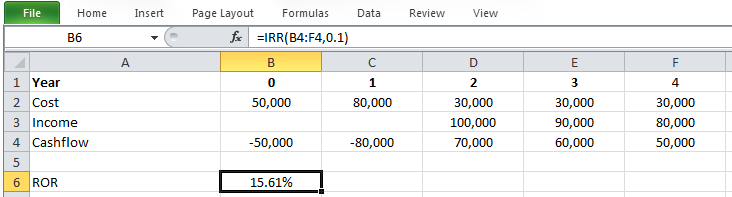
Example 5-5:
Now, assume escalation rates of 8% per year for capital cost (development cost), 12% per year for operating costs and 10% per year for revenues. Calculate ROR and NPV for this investment, and make escalated dollar analysis considering 15% escalated dollar minimum rate of return, i*.
| C0=$50,000 | C1=$80,000*(F/P8%,1) =86,400 |
Rev2=$100,000*(F/P10%,2) =121,000 OC2=30,000*(F/P12%,2) =37,632 |
Rev3=$90,000*(F/P10%,3) =119,790 OC3=30,000*(F/P12%,3) =42,148 |
Rev4=$80,000*(F/P10%,4) =117,128 OC4=30,000*(F/P12%,4) =47,206 |
|
|
||||
| 0 | 1 | 2 | 3 | 4 |
Present value of all costs = present value of all revenues
Escalated dollar ROR for this project is calculated as: i=26.24%, and it is higher than 15% escalated dollar minimum rate of return, i*. So, the project is economically satisfactory.
Since NPV at 15% escalated dollar minimum rate of return is positive, we can conclude that the project is economically satisfactory.
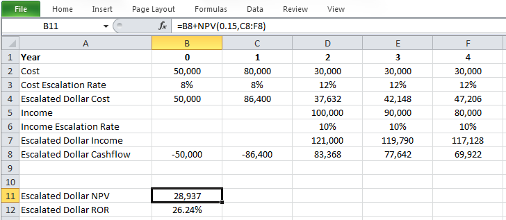
Example 5-6:
Now, consider inflation rate of 6% per year for Example 5-5 and make constant dollar analysis.
Constant dollar amounts can be calculated as:
| C0=$50,000 | C1=$86,400*(P/F6%,1) = 81,509.43 |
Rev2=$83,368*(P/F6%,2) = 74,197.22 |
Rev3=$77,642*(P/F6%,3) = 65,189.85 |
Rev4=$69,922*(P/F6%,4) = 55,385.11 |
|
|
||||
| 0 | 1 | 2 | 3 | 4 |
ROR for this project is i=19.09%,
For constant dollar analysis, it is necessary to derive constant dollar minimum rate of return, i'*, from escalated dollar minimum rate of return, i*, and inflation rate applying equation 5-2.
Therefore, the constant dollar minimum rate of return, i'*, will be 8.49%.
The constant dollar ROR for this project is calculated as 19.09%, and it is higher than i'* = 8.49%. So, the project is economically satisfactory.
In order to calculate the constant dollar NPV, we have to calculate it at a constant dollar minimum rate of return, i'*= 8.49%.
Constant dollar NPV at i'*= 8.49% is positive, so, the project is economically satisfactory.
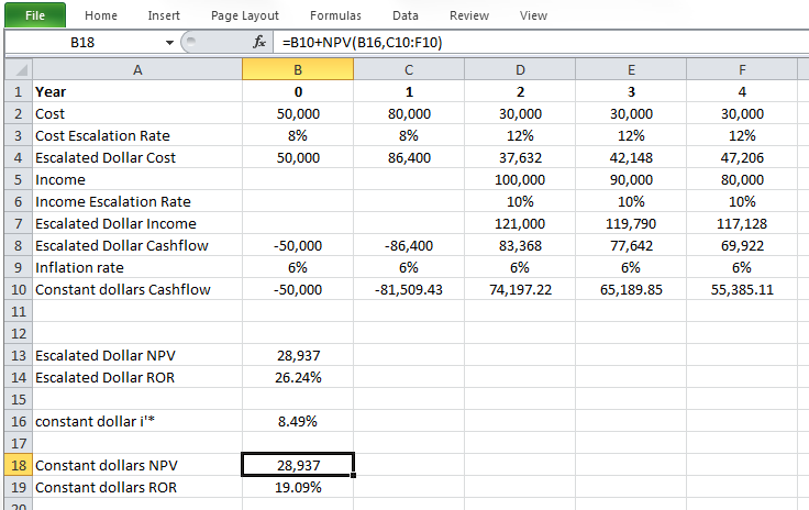
Please watch the following (17:17) video: Escalated and constant dollar ROR and NPV analysis
PRESENTER: Now let's work on a more comprehensive example. And I'm going to use an Excel spreadsheet to work on this example. And this is the data for an investment.
We are going to have investments of $50,000 and $80,000 at the present time and Year 1. We are going to have the revenues of $100,000, $90,000, and $80,000 at Year 2, 3, and 4. And the operating cost is going to be constant at $30,000 from Year 2 to Year 4.
We are going to consider the escalation rate of 8% for the capital cost and 12% for operating costs and 10% of escalation for the revenues. Let's calculate the rate of return and NPV for this investment and calculate the escalated dollar cash flow.
So because we have different escalation rates for our costs and revenue, we need to separate-- we need to keep them separate. The present time capital cost will not be affected by the escalation rate. The $80,000 of capital cost at Year 1 has to be compounded with 8%. And the compounding period is 1.
The $100 revenue at Year 2 has to be compounded by 10%, and the compounding period is 2. The operating cost at Year 2 has to be compounded by 12%, and the compounding period is 2, and so on. Payments are going to be 3 and the compounding period is going to be 4 years. The escalation rate for revenue is 10%, and the escalation rate for operating costs is 12%.
And the result.
So in order to calculate the rate of return, we write the equation for the rate of return, the present value of cost equals the present value of revenue. The present value of costs equals the present value of all capital costs and operating costs that we have here. And the present value of income equals the present value of revenue at Year 2, 3, and 4.
We could also make a summation over each column, considering the negative sign for costs, and calculate the escalated dollar cash flow and write the rate of return equation for that. Both of them are the same. And we solved the equation for i.
And we calculate the rate of return, the escalated dollar cash flow rate of return as 26.24%. So because the calculated rate of return for this project is higher than 15% escalated dollar minimum rate of return, we can conclude that this project is economically satisfactory.
So we can also calculate the NPV for this project. NPV equals the present value of all costs, considering the 15% of escalated dollar minimum rate of return, considering the negative sign, plus the present value of revenue, considering 15% of escalated dollar minimum rate of return. So we calculate the NPV as $28,937. So because this NPV is positive, we can conclude that this project is economically satisfactory.
So let me open the Excel spreadsheet and work on this example. So this is the information for this investment. These are costs. The first two ones are capital costs and the other three are operating costs. As you can see, escalation rates are different. And here, the income.
So now I'm going to calculate the escalated dollar. So for the payment, which is the capital cost at the present time, which will not be affected by the escalation rate, so it is going to be the same payment. Escalated dollar cost at Year 1 can be calculated by compounding this $80,000 by 8% and for 1 year compounding period, so it equals $80,000, multiply 1 plus 8% power 1. So this is the escalated dollar cost at Year 1.
And I can apply to the other cells. For example, the last year, which is going to be an operating cost, has to be compounded by 12% of the escalation rate and 4 compounding periods. F1, which reads it from here.
And then I'm going to calculate the escalated dollar income for our trade incomes in Year 2 to Year 4. So escalated dollar income of $100,000 equals $100,000, multiply 1 plus 10% power 2, because we are going to have two compounding periods. And I apply that to the other revenues.
And now I'm going to calculate the escalated dollar cash flow, which is going to be revenue, the escalated dollar income revenue, minus the escalated dollar cost. I don't have any revenue at the present time, so it will be 0, but I have to write that, minus the costs. And I apply this to the other years.
So this is going to be my escalated dollar cash flow. I am going to calculate the escalated dollar NPV. Because I have a payment at the present time, I have to enter that manually and then use the NPV function for the rest.
The rate was 15%. And then I will choose the cash flow, the rest of the cash flow. So this is escalated dollar NPV and the rate of return. I used the IRR function.
I choose the entire cash flow. And I enter a guess, which I just gave at 10%. And 26.24% is the escalated dollar rate of return.
So this is the escalated dollar cash flow that we just calculated. Now let's consider an inflation rate of 6% per year for this escalated dollar cash flow. And let's calculate the constant dollar cash flow. And then, let's calculate the rate of return and NPV for constant dollar cash flow.
In order to calculate the constant dollar cash flow, we need to discount each payment by the inflation rate, a 6% inflation rate, considering the discounting period. For example, the escalated dollar of $86,400 at Year 1 has to be discounted by 6%, and the discounting period, which is going to be 1, and so on. For Year 2, the discounting period is 2, 6% inflation rate, and so on. And the results.
So this is going to be our constant dollar cash flow. We write the rate of return equation. And we solve the equation for i. And we calculate the constant dollar rate of return as 19.09%.
Now let's calculate the NPV for constant dollar cash flow. But a very important thing here is what rate should be used to calculate the NPV for constant dollar cash flow? We know that the escalated dollar minimum rate of return is 15%. But we cannot use the escalated dollar minimum rate of return for constant dollar NPV calculations.
So what should we do here? We can use the Fisher equation to convert the escalated dollar minimum rate of return into the constant dollar minimum rate of return using the inflation rate. So here is the Fisher equation.
This 15% is an escalated dollar minimum rate of return and a 6% interest rate. The result is going to be 8.49%, which is going to be the constant dollar minimum rate of return. This is the rate that we have to use for calculating our constant dollar NPV.
So we use the constant dollar minimum rate of return of 8.49% to calculate the NPV of constant dollar cash flow. And this is the NPV of constant dollar cash flow. And you can see because this is positive, we can conclude the project is economically satisfactory.
We calculated the constant dollar rate of return as 19.09%. And we need to compare this with the constant dollar minimum rate of return of 8.49% that we just calculated. And because this rate of return is higher than this minimum rate of return, we can also conclude that this project is economically satisfactory.
Now let me open the Excel spreadsheet again. So this is the escalated dollar cash flow. And we are going to consider the 6% of inflation rate for this escalated dollar cash flow. And then we have to calculate the constant dollar cash flow.
In order to calculate the constant dollar cash flow, we need to discount each payment by 6% and the discounting period. So we can leave it as it is, $50,000 of costs. But this escalated dollar cash flow has to be discounted by 1 plus 6%, our discounting period. And then I can apply this to the other years. So for example, the last year, constant dollar cash flow in the last year equals the escalated dollar divided by 1 plus inflation rate power the year.
Now let's calculate the constant dollar NPV. But in order to calculate the constant dollar NPV, we need the constant dollar minimum rate of return. How do we calculate that? I will use the Fisher equation, escalated dollar minimum rate of return, and the inflation rate to calculate the constant dollar minimum rate of return.
So constant dollar minimum rate of return, or i prime star, equals 1 plus 15%, which was escalated dollar minimum rate of return, divided by 1 plus inflation rate, 6%, minus 1, which equals 8.49%. So this 8.49% is the constant dollar minimum rate of return that I can use to calculate the constant dollar NPV.
So I have the constant dollar cash flow here. I have a constant dollar minimum rate of return here. And I can calculate the constant dollar NPV.
So the payment at the present time, I have to enter that manually, plus the NPV function. The rate is a constant dollar minimum rate of return and the rest of the constant dollar cash flow. So because this NPV is positive, I can conclude that the constant dollar cash flow of the project with this constant-dollar cash flow is a good project to invest.
And let's calculate the constant dollar rate of return, which is a fairly straightforward, IRR function. I choose the constant dollar cash flow. I give it a guess, 10%. And this is the constant dollar rate of return, which is 19.09%. And because this constant-dollar rate of return is higher than the constant dollar minimum rate of return, I can conclude that this project is economically satisfactory in terms of rate of return.
So you can also use the Fisher rule to calculate the constant dollar rate of return. Keep it in your mind. It's a very good double-check method to make sure your final result is correct.
So we have the constant-- we have the escalated dollar rate of return here. We have an inflation rate of 6%. So with these two, I should be able to calculate the constant dollar rate of return using the Fisher rule.
So let's see. So the constant-dollar rate of return using the Fisher equation is 1 plus escalated dollar rate of return divided by 1 plus inflation rate of 6% minus 1. And it should give me the exact same value as this rate of return that I calculated here. As you can see, it will be the same.
Summary of calculations:
- Step 1: Calculating escalated dollar cash flow using escalation rate and F/P factor
- Calculating escalated dollar ROR from calculated escalated dollar cash flow in step 1
- Calculating escalated dollar NPV from calculated escalated dollar cash flow in step 1 and given escalated dollar minimum rate of return, i*
- Step 2: Calculating constant dollar cash flow using the given inflation rate and P/F factor from the calculated escalated dollar cash flow in step 1
- Calculating constant dollar ROR from calculated constant dollar cash flow in step 2
- Calculating constant dollar minimum rate of return, i'*, from given escalated dollar minimum rate of return, i*, and given inflation rate, f, using Fisher equation
- Calculating constant dollar NPV from calculated constant dollar cash flow in step 2 and calculated constant dollar minimum rate of return, i'*
Note that the constant dollar NPV is identical to the escalated dollar NPV. Constant NPV equations are mathematically equivalent to escalated dollar NPV equations and then give the same results.
Note that Example 5-4 implicitly assumes the escalation rate is 0% per year. So, for NPV and ROR analysis in Example 5-4, we need to consider a 15% escalated dollar minimum rate of return.
And since it is positive, the project is economically satisfactory.
And calculated ROR (15.61%) is also higher than the 15% escalated dollar minimum rate of return, so we can conclude that the project is economically satisfactory.
Summary and Final Tasks
Summary
Escalated values are also defined as actual, current, then current or nominal dollars. They are always inclusive of the effects of inflation and other parameters including technological, environmental, market, and related issues.
Constant values are escalated values that have had the effects of inflation discounted from them to a base period in time which typically is time zero, but could be any point. Constant dollars are also referred to as real or deflated dollars.
The only difference between escalated and constant values is the inflation rate each year related to the host currency. Consideration of this difference is critical for general geo-resource project evaluation.
Reminder - Complete all of the Lesson 5 tasks!
You have reached the end of Lesson 5! Double-check the to-do list on the Lesson 5 Overview page [36] to make sure you have completed all of the activities listed there before you begin Lesson 6.
Lesson 6: Uncertainty and Risk Analysis
Introduction
Overview
In this era of advancing technology, successful managers need to make investment decisions that determine the future success of their companies by drawing systematically on the specialized knowledge, accumulated information, experience, and skills of many people. In previous lessons, the investment analyses were all considered to be made under "no-risk" conditions. In this lesson, we add in the uncertainties when evaluating an energy/mining project. The objective of investment decisions is to invest available capital where we have the highest probability of generating the maximum possible future profit. The use of quantitative approaches to incorporate risk and uncertainty into analysis results may help us be more successful in achieving this objective over the long run.
Learning Objectives
At the successful completion of this lesson, students should:
- understand how to conduct sensitivity analysis to analyze the effects of uncertainty;
- be able to conduct expected value analysis; and
- understand the risk due to natural disasters.
What is due for Lesson 6?
This lesson will take us one week to complete. Please refer to the Course Syllabus for specific time frames and due dates. Specific directions for the assignment below can be found within this lesson.
| Reading | Read Chapter 6 of the textbook. |
|---|---|
| Assignment | Homework and Quiz 6. |
Questions?
If you have any questions, please post them to our discussion forum, located under the Modules tab in Canvas. I will check that discussion forum daily to respond. While you are there, feel free to post your own responses if you, too, are able to help out a classmate.
Risk Analysis
So far, in previous lessons, effect of risk and uncertainty haven’t been considered in our economic evaluations and the analyses were assumed to be of no-risk condition. In this case, the probability of success and achieving anticipated results is assumed to be 100%, but in reality, some degree of uncertainty is involved and this probability is much lower. The economic analyses that don’t include risk and uncertainty are based on “best guess,” and the results aren’t highly accurate and reliable. For example, if a study shows 20% and 25% ROR for project A and B, the manager would probably choose project B over A. But what if the probability of success is 90% for project A and 40% for project B? This example shows how important it is to consider the effect of risk and uncertainty as a component in economic evaluations.
Quantitative methods, along with informal analysis, are used for decision making under risk and uncertainty. Quantitative methods aim to provide the best possible set of information to decision-makers so that they may apply their experience, intuition, and judgment to achieve the final decision; the decision that leads to maximum possible future profit with the highest probability. There are several different approaches that can be used to quantitatively incorporate risk and uncertainty into analyses. These include sensitivity analysis or probabilistic sensitivity analysis to account for uncertainty associated with possible variation in project parameters, and expected value or expected net present value or rate of return analysis to account for risk associated with a finite probability of failure. The use of sensitivity analysis is advocated for most economic analyses and the use of expected value analysis is advisable if a finite probability of project failure exists. Sensitivity analysis is a means of evaluating the effects of uncertainty on investment by determining how investment profitability varies as the parameters are varied that effect economic evaluation results.
Sensitivity analysis can show how results change if the input parameter changes. If we change one input parameter (such as initial investment) and the result (such as NPV of the project) varies significantly in a wide range, then we say the result is sensitive to the specified input parameter. Here, we aim to find the most sensitive variables. The input parameter investigated for sensitivity analysis usually includes initial investment, selling price, operating cost, project life, and salvage value. If probabilities of occurrence are associated with various levels of each investment parameter, sensitivity analysis becomes probabilistic sensitivity analysis.
It may now be evident to you that the term “uncertainty” as used in this lesson refers to possible variation in parameters that effect investment evaluation. “Risk” refers to the evaluation of an investment using a known mechanism that incorporates the probabilities of occurrence for success and failure and/or of different values of each investment parameter. Both uncertainty and risk influence almost all types of investment decisions, but especially investment involving research and development for any industry and exploration for minerals and oil or gas.
Please watch the following video (3:24): Risk, Uncertainty, and Sensitivity Analysis.
PRESENTER: In this video and the next videos, I will explain how to incorporate risk and uncertainty in the economic evaluation of projects for the purpose of investment. I will explain how we can apply the sensitivity analysis techniques to evaluate the project in this case. In previous lessons, in previous videos, we use fixed numbers. All the numbers that we used were deterministic at no risk condition. The probability of achieving an outcome was 100%.
But it is not the case in real life. There is always some level of uncertainty in the anticipated result, especially things that are happening in the future. For example, if an evaluation of two projects, Project A and Project B shows that Project A has a rate of return of 20% and Project B has a rate of return of 25%, assuming they have the same skill and they require the same amount of investment, what would you do as a manager?
You would choose the project with a higher rate of return. So you will choose Project B, which has a higher rate of return. But what if I tell you the probability of success in Project A is 90% and the probability of success in Project B is just 40%? What would be your decision?
Decision-makers use combinations of qualitative and quantitative methods in risk situations. In this video, we are focusing on quantitative methods. Quantitative methods are aiming to provide the best possible information for the decision-maker. And in the end, decision-makers have to use their own experience, intuition, and judgment for the final decision about maximum possible profits in the future with the highest probability.
There are several quantitative methods for incorporating risk and uncertainty. I will explain two of these methods in this video and the following videos. The first one is called sensitivity analysis or probabilistic sensitivity analysis. And the next one is going to be expected value or expected net present value.
Sensitivity analysis is a method that helps us understand the sensitivity of results to the input variables. Here, our result, our evaluation result, is a measure that shows us the profitability of the project, which it is NPV, rate of return, or any other parameter that we learned so far. In a sensitivity analysis, we want to determine how results vary if we change input variables. What would be the magnitude of change in one variable with respect to the change in other variables? Sensitivity analysis helps decision-makers to find the parameters that have the biggest impact on the results.
Italicized sections are from Stermole, F.J., Stermole, J.M. (2014) Economic Evaluation and Investment Decision Methods, 14 edition. Lakewood, Colorado: Investment Evaluations Co.
Uncertainty and Sensitivity Analysis
As explained before, in sensitivity analysis, we aim to discover the magnitude of change in one variable (here, output variables) with respect to change in other variables (here, input parameters). Then, we can rank the variables based on their sensitivity. It helps the decision-maker to understand the parameters that have the biggest impact on the project.
The following example introduces a single variable sensitivity analysis. Please note that here we assume variables are independent and have no effect on each other. For example, it is assumed that the magnitude of initial investment doesn’t affect the operating costs.
Example 6-1:
For a project, the most expected case includes an initial investment of 150,000 dollars at the present time, an annual income of 40,000 for five years (starting from the first year), and a salvage value of 80,000. Evaluate the sensitivity of the project ROR to 20% and 40% increase and decrease in initial investment, annual income, project life, and salvage value.
Before-tax cash flow of this investment can be shown as:
|
-$150,000
|
$40,000
|
$40,000 | $40,000 | $40,000 | $40,000 |
$80,000
|
|
|
||||||
|
0
|
1
|
2
|
3
|
4 |
5
|
|
The most expected ROR based on the most expected initial investment, annual income, and salvage value can be calculated as:
The most expected ROR will be 20.5%.
A) Sensitivity Analysis of initial investment
| Initial investment | Change in prediction | ROR | Percentage change in 20.5% ROR prediction |
|---|---|---|---|
| 90,000 | -40% | 43.5% | 112.7% |
| 120,000 | -20% | 29.6% | 44.8% |
| 150,000 | 0 | 20.5% | 0% |
| 180,000 | 20% | 13.8% | -32.6% |
| 210,000 | 40% | 8.6% | -57.8% |
As you can see, changes in ROR with respect to changes in initial investment are considerably high. In general, parameters that are close to time zero have a higher impact on the ROR of the project.
B) Sensitivity Analysis of project life
| Project life | Change in prediction | ROR | Percentage change in 20.5% ROR Prediction |
|---|---|---|---|
| 3 | -40% | 12.9% | -36.6% |
| 4 | -20% | 17.7% | -13.5% |
| 5 | 0 | 20.5% | 0% |
| 6 | 20% | 22.2% | 8.7% |
| 7 | 40% | 23.4% | 14.5% |
Note that changes in the project ROR become smaller as the project life gets longer.
C) Sensitivity Analysis of annual income
| Annual income | Change in prediction | ROR | Percentage change in 20.5% ROR prediction |
|---|---|---|---|
| 24,000 | -40% | 8.1% | -60.6% |
| 32,000 | -20% | 14.3% | -30.0% |
| 40,000 | 0 | 20.5% | 0% |
| 48,000 | 20% | 26.5% | 29.5% |
| 56,000 | 40% | 32.4% | 58.5% |
Changes in annual income also have a significant effect on ROR because these changes start happening close to present time.
D) Sensitivity Analysis of salvage value
| salvage value | Change in prediction | ROR | Percentage change in 20.5% ROR prediction |
|---|---|---|---|
| 48,000 | -40% | 17.0% | -17.0% |
| 64,000 | -20% | 18.8% | -8.2% |
| 80,000 | 0 | 20.5% | 0% |
| 96,000 | 20% | 22.0% | 17.7% |
| 112,000 | 40% | 23.5% | 14.8% |
We can conclude that salvage value has the least effect on the ROR of the project because salvage value is the last amount in the future and its present value is relatively small compared to other amounts.
The following figure displays a tornado chart that is a very useful method to graphically summarize the results of sensitivity analysis. The right and left hand side of each bar indicate the maximum and the minimum ROR that each parameter generates when changed from -40% to +40%.
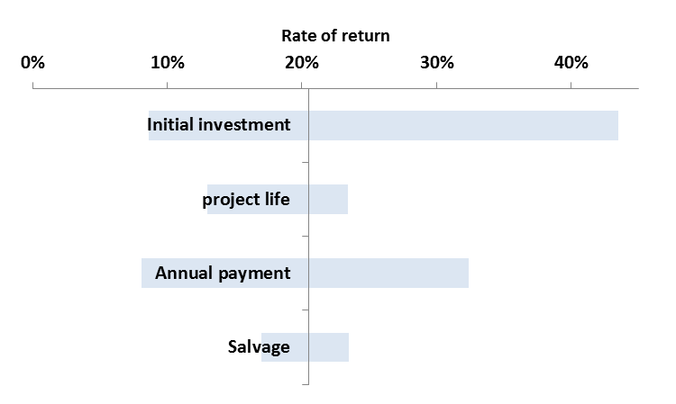
| Type | Rate of Return Range |
|---|---|
| Initial investment | 8.6% - 43.5% |
| Project life | 13% - 23.4% |
| Annual payment | 8.1% - 32.4% |
| Salvage | 17% - 23.5% |
Please watch the following video (18:02): Sensitivity Analysis.
PRESENTER:
In this video, I will work on an example and explain the sensitivity analysis method. I will describe how we can use this method for project evaluation. Let's work on a simple example.
In this example, we will run single variable sensitivity analysis. We also assume all the input variables are independent and have no effect on each other. For instance, we assume the magnitude of initial investment has no effect on operating costs.
This investing project requires $150,000 of investment at the present time and it yields the annual income of $40,000 for five years from year one to year five and the salvage value of $80,000 in the end of the year five. And we want to evaluate the sensitivity of the project rate of return to 20% and 40%, change increase and decrease in initial investment, annual income, project life, and salvage.
First we calculate the rate of return on this cash flow for this project. The present value of costs equals present value of income plus present value of salvage. And we will find that we will solve this equation for i using the IRR function in Excel or any other spreadsheet. And we calculate the rate of return on this cash flow as 20.5%.
First, sensitivity analysis of initial investment. So in the first step, we want to see what would be the rate of return for this project if we decrease the initial investment by 40%. It means we have to multiply this under $50,000 by 1 minus 40%. So it is going to be $90,000. So if the initial investment of the project decreases by 40%, then we will have the initial investment of $90,000 at present time.
And we calculate the rate of return for this new situation. Present value of cost equals present value of income plus present value of salvage. And we calculate the rate of return as 43.5%.
Now effect of 20% decrease in the initial investment. So the initial investment, if it is decreased by 20%, is going to be 1 minus 20%, multiply $150,000. And we calculate the rate of return for the new situation, for the case that we have 20% less initial investment. And the rate of return is going to be 29.6%.
The third case is when we calculate the rate of return for a 20% increase in initial investment. So initial investment is going to be 1 plus 20%, multiply $150,000, which is going to be $180,000 of investment. And the rate of return can be calculated as present value of cost equals present value of income plus present value of salvage. And the rate of return will be 13.8% if the initial investment is increased by 20%.
And the fourth case is when our initial investment is increased by 40%, which is going to be 1 plus 40%, multiply $150,000, which comes to $210,000. And the rate of return is calculated as 8.6% if the initial investment is increased by 40%.
And this table summarizes the result for sensitivity analysis on initial investment. So the third row is the base case when there is no change in our initial investment. The rate of return, as we calculated, was 20.5%. If the initial investment is decreased by 40%, then the rate of return for this project is going to be 43.5%, which will be 112.7% higher than the base case that we had.
Initial investment is decreased by 20%, then the rate of return is going to be 29.6%, which, comparing to the base case, the rate of return is going to be 44.8% higher than the base case. If the initial investment is increased by 20%, then rate of return is going to be 13.8, which is going to be around 33% lower than the base case. And the last case, if the initial investment is increased by 40%, then the rate of return for the project is going to drop to 8.6%, which is 58% lower than the base case that we had.
Now let's do the sensitivity analysis for the project lifetime. The project lifetime is initially five years. So the 40% decrease in project lifetime is going to be 1 minus 40, multiply 5, which is going to be three years. So the project with the initial investment of-- we hold every other thing constant. So the project with initial investment of $150,000 and annual income of $40,000 for three years and the salvage value of $80,000. We calculate the rate of return, which is going to be 12.9%.
And then effects of a 20% decrease in project lifetime. So if the project lifetime is decreased by 20%, you're going to have four years, 1 minus 20% multiply by five, which comes to four. And a calculation of rate of return for the new cash flow, we're going to have four years of income of $40,000. And rate of return is going to be 17.7%
Of 20% increase in project life, which is going to be 1 plus 20%, multiply 5, which is going to be 6 year. One year increase in project lifetime, in this case, we are going to have a rate of return of 22.2%. And if the project lifetime is increased by 40%, meaning that we add two more years to the lifetime of the project, one plus 0.4, multiply 5, equals to 7. We have two more years of project lifetime. And the rate of return can be calculated as 23.4.
And we summarize the sensitivity analysis of project life result in this table. So the third row is the base case. Project life is initially five years. And the rate of return is 20.5%.
If the project life is decreased by 40%, we are going to have three years of project life and the rate of return is going to be 12.9%. If the project life is decreased by 20%, then the rate of return is going to be 17.7%, which is 13.5% less than the base case. If the project life is increased by 20%, then we can see it is going to have positive impact on the rate of return, which is 8.7% higher than the base case, higher than 20.5%. And if the project lifetime is increased by 40%, the project life is going to be seven years and the rate of return is going to be 23.4, which is 14.5% higher than the base case, which was 20.5%.
And now sensitivity analysis for annual income. The initial value for annual income was $40,000. 40% decrease means 1 minus 40%, multiply $40,000, and we're going to have the annual income of $24,000. We calculate the rate of return for such projects. So every other thing is the same. We just decrease the annual income by 40%. So the rate of return is going to be 8.1%. [AUDIO OUT].
The effect of 20% decrease in annual income will be 1 minus 20%, multiply $40,000, which is going to be $32,000. We're going to have $32,000 if the annual income is decreased by 20%. And the rate of return for such project is going to be 14.3%.
We will repeat these calculations for 20% increase in annual income. If annual income from the base case is increased by 20%, we are going to have 1 plus 20%, multiply $40,000, which gives $48,000 of annual income per year for five years. And the rate of return is going to be 26.5%.
We'll repeat the calculations for a 40% increase in annual income, which is going to be 1 plus 40%, multiply $40,000, which comes to $56,000 annual income. So if our annual income is increased by 40% from the base case, we are going to have $46,000 per year. And the rate of return in this new case will be 32.4%.
So, again, this table summarizes the sensitivity analysis of annual income. The base case is when we have $40,000 of income per year. The rate of return is going to be 20.5%. If the annual income is decreased by 40%, we are going to have $24,000 per year and the rate of return is going to be 8.1%, which is going to be 60.6% lower than the base case, lower than the base case of 20.5%.
If the annual income is decreased by 20%, we are going to have $32,000 per year and the rate of return is going to be 14.3%, which is almost 30% less than the base case. If annual income is increased by 20%, we are going to have $48,000 dollars per year and the rate of return is going to be increased to 26.5%, which is 29.5% percent higher than the base case. And in the end, if annual income is increased by 40%, we will have the annual income of $56,000. And rate of return is going to be 32.4%, which is 58.5% percent higher than the base case.
And the last part, we are on the sensitivity analysis for the salvage value. The initial value for salvage is $80,000. 40% decrease in salvage value can be calculated as 1 minus 40%, multiply $80,000, which comes to $48,000. And the rate of return for this change, $40,000 of salvage, which is here, is going to be 17%.
We'll repeat the calculations for 20% decrease in salvage. 1 minus 20%, multiply $80,000, which is going to be $64,000 of salvage. And the rate of return, 18.8%. Percent.
We will calculate this for 20% increase in salvage. 1 plus 20%, multiply $80,000 equals $96,000. And the rate of return can be calculated as 22%. And the last one, 40% increase in salvage value, which will be 1 plus 40%, multiply $80,000, equals $112,000 of salvage value. And rate of return will be 23.5.
This table summarizes the sensitivity analysis of salvage value. The third row is the base case. There is no change in any input variable and the rate of return is 20.5%.
The first row is the case that we have 40% decrease in salvage value. In this case, the rate of return is going to be 17%, which is 17% lower than the base case, which was 20.5%. If the salvage value is decreased by 20%, then rate of return is going to be 18.8%, which is 8.2% lower than the base case.
If the salvage value is increased by 20%, the rate of return is going to be 22%, which is 7% higher than the base case. Last row, which shows the 40% increase in salvage. And the rate of return in this case is going to be 23.5%, which is almost 15% higher than the base case of 20.5%.
This table summarizes the sensitivity analysis result for these four input variables. So the second row is the base case where nothing has changed. So rate of return is 20.5%.
The first row shows if the input is decreased by 40%. So if the initial investment is decreased by 40%, then rate of return is going to be 43.5%. If the project lifetime is decreased by 40%, we can see it has a negative effect on the rate of return. The rate of return is going to decrease to 12.9% and so on.
The last row shows the result if the input variable is increased by 40%. So if the initial investment is increased by 40%, rate of return is going to be 8.6%. If the project life is increased by 40%, rate of return is going to be 23.4 and so on.
We can also summarize these results in a graph called tornado graph. And we can see here this vertical line shows the base case where nothing has changed. The rate of return is 20.5%. This bar shows what would be the change in the rate of return of the project if initial investment changes from 40% positive to 40% negative, 40% increase to 40% decrease.
Credit: Farid Tayari
If you are interested, the following video (10:48) explains how to draw a tornado chart in Microsoft Excel (please watch from 6:10 to 9:00).
CHARLIE NUTTELMAN: This screencast is going to go over a sensitivity analysis, and we're going to generate a tornado plot. A sensitivity analysis is basically a study into how sensitive is the process, so the process outputs, to the inputs. So just as an example here, we have a process, and it's got a bunch of inputs, and it may have one or more outputs.
An example might be a reactor where the inputs would be things like the temperature, the pressure, maybe the size, the flow rate, concentration of different things, and so on. And the outputs might be conversion. Just a simple example. And we want to determine how sensitive the outputs of the process are to the inputs.
The specific example I'm going to be working with has to do with net present value. We've made a screencast on this already, and you don't necessarily have to understand this net present value example. It has to do with engineering economics and determining the net present value of a venture 15 years from the current time. We have different inputs to the process. The inputs would be things like the cost of land, the cost of royalties per year, the total depreciable capital-- that's how much you have to invest in major equipment-- working capital, startup costs.
We have sales, which is S. Other inputs include tax, because tax rates might change. And cost of sales, here we have 6 million. And we have an interest rate, or the cost of capital. So again, you don't necessarily have to understand exactly what I've done in this spreadsheet to understand sensitivity analysis. The important thing is that we have a process and we have multiple inputs that go into determining what the output is. And for this process, the output is down here.
This tells us that the net present value of a venture based upon our base case, or our baseline or nominal values of these different variables up here, the net present value that is about 58 million. We're going to now do a sensitivity analysis. We're going to see what happens when we change different values here for the cost of land, maybe the annual sales, and annual costs, and so on. So what happens, maybe, if we subtract 20% from the nominal values and increase 20%?
So you'll notice here, I have 58.78 million down here. And if I change something like cost of sales, let's just say to eight, instead of being 58.78, it's a lot less. It's 50.30. So you can see that this process, the output which is net present value, depends upon the input variable. So I'm going to put that back to six. And maybe I change land to instead of 5 million, it's negative 4 million but that didn't change it a whole lot. It was 58.78, and now it's 59.78. So I'm going to put that back to minus five.
We're going to do a data table to look at these different input variables and what effect they have on the output. So we're going to do a sensitivity analysis first on the working capital. The nominal value, or the baseline value, for working capital is negative 20 million. That's how much we're going to request for working capital. And we want to ask ourselves how sensitive is the net present value after 15 years? How sensitive is that to the working capital? So if we have 80%, that'd be minus 16 instead of minus 20, as opposed to 120%, which is negative 24.
So all I've done here is multiply our baseline value of negative 20, which is up here in our spreadsheet. I multiplied that by 80%, all the way up to 120%.
We're going to make a data table here. When you make a data table, we have a column of different inputs that we're going to do kind of a case study on, the cell one up and one over from our values. This is a pointer formula, so I'm going to do equals. We're pointing to our net present value. That's the result. And then what I can do is highlight all of this, our column of cells, plus one row above. And I'm going to go into Data, What If Analysis, Data Table. And this is a column data table. And each of these working capital values is going to be placed into cell B4 up here.
And so I'm going to press OK, and it's going to do sort of a case study on that. I forgot to mention one thing. If I just did a multiplication of cell C33 here, which is negative 20, times the percentage and created a vector here, I actually have to copy and paste so that's not a formula. Because if this is a formula and we put that into the data table, it doesn't quite work right. So we have to copy and paste the values so they're just numbers instead of formulas in this column before we do the data table.
So this is telling us if the working capital is negative 16, the net present value is about 62.5 million. And if we increase it by 20%, we see that the net present value is about 55 million. So I can go through all of these different values. And the green here represents the baseline values. So we have working capital, which I showed you. I did this for startup costs, sales, the interest rate or cost of capital, the land costs, total depreciable capital, capital, and cost of sales.
And what I've done for all of these, I've taken the minus 20, which is our 80% of nominal cost, and our 120% of that particular variable and I've made a summary table here. What we're going to do now is create something known as a tornado plot. To create the tornado plot, I'm going to highlight one of these rows. I go up here to Insert, Chart, and we're making a clustered chart, a clustered bar chart. And right now, it's not looking anything like a tornado plot, but bear with me here.
I'm going to format this a little. I'm going to go over here and add in axis titles. I'm going to add in a legend. I'm going to go back up here, and I'm going to copy, so I'm selecting this, Control + C. That's the 120%. And I'm going to click in the area, do Control paste. Now, again, this isn't looking really like a tornado plot, but we have some work to do. We need to change this. I'm going to do Format Axis, and it's going to cross axis values. Vertical axis crosses axis value at 58.78. That was our nominal value.
So if I go back up here, 58.78 is the net present value when we have 100% of all those values. That was our base case. Now this is sort of looking like a tornado diagram. And I'm going to click on one of these series, Format Data Series. We're going to do 100% overlap, sort of eclipsing. And I'm going to make this a little bigger. I'm going to decrease the gap width, maybe something around 60%.
We can further modify this. So I'm going to right-click on this axis, Format Axis. Let's change the number to be zero decimals. I'm also going to click on the category over here, and we will format that. So I'd right-click on this, format that axis. I'm going to change the labels so they are low. What that does is it brings those labels to the left side.
And another thing I'm going to do is change those labels. So I'm going to do Select Data. Instead of these one, two, through eight, I'm going to edit that, and that's going to be named our categories up here. So I can do that. Click OK. And it has added those different categories.
And the last thing we need to do is to change our legend. So I'm going to bring the legend inside here so I can expand this a tiny bit. And I can right-click in here and do Select Data. And I'm going to change this to minus 20%. I'm editing the series, and this will be plus 20%. And we're pretty much done. So that is a tornado diagram.
And what this tornado plot shows us is that if we change, for example, sales, if that goes down by 20% of our baseline, then that has a huge effect on the net present value. Same thing with if we increase sales by 20%. That has a very big effect on net present value. Some other things that don't have as big of effect, you see that C_land doesn't have a big effect. If your land costs vary tremendously, that's not going to have a huge effect on net present value at all. But if your sales are off of what you're anticipating, then this can have a huge effect on the net present value.
So that's varying from around 20 million to 100 million, which is a huge difference there. And your boss might say, if you gave him this sensitivity plot, your boss might say, well, we need to put a lot more effort into making sure we have a really good estimate on sales. Because if sales are 20% lower than what we're expecting, then the profitability of this venture's way lower than if our sales are 20% higher than what we're expecting.
This sort of tells you what are the main players in your output, and the output, in this case, is net present value. And if you really wanted to, you could organize this. You can put the big bars up at the top and the small ones at the bottom, and it sort of looks like a tornado, so that's what the tornado plot gets its name. OK, thanks for watching this screencast.
Expected Value Analysis (Economic Risk Analysis)
The expected value is defined as the difference between expected profits and expected costs. Expected profit is the probability of receiving a certain profit times the profit, and the expected cost is the probability that a certain cost will be incurred times the cost.
Example 6-2:
A wheel of fortune in a gambling casino has 54 different slots in which the wheel pointer can stop. Four of the 54 slots contain the number 9. For a 1 dollar bet on hitting a 9, if he or she succeeds, the gambler wins 10 dollars plus the return of the 1 dollar bet. What is the expected value of this gambling game? What is the meaning of the expected value result?
- 0.185 dollars indicates that if the gambler plays this game over and over again, the average gain for the gambler per bet equals - 0.185 dollars, which means the gambler will lose 0.185 dollars per bet. Note that for a satisfactory investment, a positive expected value is a necessary, but not sufficient, condition.
Example 6-3:
Assume drilling a well costs 400,000 dollars. There are three probable outcomes:
a) 70% probability that the drilled well is a dry hole
b) 25% probability that the drilled well is a producer well with such rate that can be sold immediately at 2,500,000 dollars
c) 5% probability that the drilled well is a producer well with such rate that can be sold immediately at 4,000,000 dollars
Calculate the project's expected value.
Note that +425,000 dollars is a statistical term; it means the average of +425,000 dollars will be achieved in the long-term for drilling over and over again in a repeated investment of this type.
Expected NPV and Expected ROR Analysis
Example 6-4:
Assume a research project that has the initial investment cost of 100,000 dollars. There are two possible outcomes:
a) 30 % success: that leads to an annual profit of 60,000 dollars for five years (starting from year 1) with a salvage value of zero
b) 70 % failure: that leads to annual profit and salvage value of zero
Considering a minimum 12% discount rate, compare the expected NPV, and explain if this investment is satisfactory.
| 30 % success: | -$100,000 | $60,000 | $60,000 | $60,000 | $60,000 | $60,000 |
| 70 % failure: | -$100,000 | 0 | 0 | 0 | 0 | |
|
|
||||||
| 0 | 1 | 2 | 3 | 4 | 5 | |
Since considering risk in calculations results in negative expected Net Present Value (ENPV), it can be concluded that this investment is expected to be economically unsatisfactory. Note that risk-free NPV (assuming 100% success probability) shows good and economically satisfactory results.
Example 6-5:
Calculate the expected Rate of Return for the above example.
Expected ROR is the “i” that makes Expected NPV equal 0.
Expected Present worth income @ "i" – Present Worth Cost @"i" = 0
By trial and error, Expected ROR = - 3.4%
Note that risk free ROR shows a satisfactory result.
Risk-free ROR = 52.8%, which is much higher than the minimum ROR.
Another way to calculate the expected ROR, which is similar to the previous method, is to calculate expected cash flow and then find the ROR for that.
Expected cash flow can be determined by multiplying each scenario’s cash flow by its probability and then make summation over each year:
| Year 1 | Year 2 | Year 3 | Year 4 | Year 5 | |
|---|---|---|---|---|---|
| Expected cash flow |
Then:
| Year 1 | Year 2 | Year 3 | Year 4 | Year 5 | |
|---|---|---|---|---|---|
| Expected cash flow | -$100,000 | $18,000 | $18,000 | $18,000 | $$18,000 |
By trial and error, Expected ROR = - 3.4%
Please watch the following video (14:01): Expected Value Analysis, Part I.
PRESENTER: In this video, I will explain the second method to incorporate risk and uncertainty in project evaluations. This method is called expected value analysis, and the expected value is the difference between expected profits and expected costs. Expected profit is the probability of receiving a profit multiplied by the profit, by the payoff, and the expected cost is the probability that certain costs will be incurred multiplied by that cost.
Let's assume a wheel of fortune that has 24 slots, and three of these slots have a red color. So you randomly turn this wheel of a slot, and if you get a red color, you will win $5. And if you get any color other than red, you will lose $1. So let's see what would be the expected value of this game and what is the meaning of the expected value results?
So the probability of success is 3/24, and the probability of failure is going to be 21 divided by 24. So the expected value equals the expected value of profit minus the expected value of cost. The expected value of this game is minus $0.25. So it means that if we play this game over and over again, the average gain per bet, the average gain per game, is going to be $0.25. So if we play this game over and over again, we will lose $0.25 per game.
Let's work on this example. Assume a drilling well that costs $400,000, and there are three possible outcomes. We have a 70% probability that we get a dry hole, which means there will be no outcome and we just have the cost of $400,000 at the present time. There is a 25% probability of success that we get a producer well, which can be immediately sold at a price of $2.5 million. And we have a 5% probability that we drill a well that is a producer and can be sold immediately at $4 million.
Let's calculate the project's expected value. So this is the expected value of failure, 70% multiplied by we have just $400,000 of cost. There is no income revenue or profit, in this case. And we have two cases of success. We have 25% of success that we get a producer well and we can sell it at $2.5 million, but we still have the $400,000 of costs. And also, we have another success case with a probability of 5% that is going to yield $4 million of immediate income, and we have $400,000 of drilling cost.
And the summation is going to be $425,000, the expected value of this project. So in each case, we multiply the probability of that event by the outcome of that event. So this is the outcome. This is the failure case. This is the outcome of the failure, and this is the probability. Here, this is one of the success cases. This is a 25% probability of success. And in case of success, we are going to have $2.5 million, but still, we have to pay the drilling cost and so on.
Please note that the $425,000 of expected value for this project is a statistical term, and it means that the average of $425,000 will be achieved in the long term. If we do this drilling, if we play this game, if we drill this field over and over again, holding the probabilities and costs and incomes constant, this is the expected value that we are going to achieve after doing the drilling again, over and over again.
Another example. Let's assume an investment project requires the initial investment cost of $100,000, and there are two possible outcomes. There is 30% of success that leads to an annual profit of $60,000 for five years, equal payments of $60,000 for five years. The salvage value is going to be zero. And the 70% failure that we receive nothing. There is no annual profit, and salvage would be zero.
Let's calculate the expected NPV for this project, assuming the minimum discount rate of 12%. So we draw these two cases in the timeline. There is 30% of success that we have $100,000 of cost at the present time. And in this case of success, we are going to have a $60,000 annual income of $60,000 per year from year one to year five. In case of failure, we still need to pay the initial costs for this project, but we will earn nothing in the future years.
So in this case, we need to calculate the NPV of each case, multiply that by the probability, and then make a summation over all the possible cases. So here we have a 30% probability of success. This is the NPV of success. This shows the NPV of success. We have $100,000 of cost at the present time, and we have five equal payments of $60,000 from year one to year five.
Probability of failure. Multiply the failure case, NPV of failure, which is going to be just the $100,000 of cost at the present time, and the expected NPV for this project, which is a negative value.
So if we consider risk in this project, meaning that we are assuming a 30% probability for success and 70% probability for failure, we are going to have expected-- We are going to have negative expected NPV, which means that this project is not a good project for investment. Note that the risk-free NPV, meaning that the probability of success is 100%, is going to be a positive number, which means this project is economically satisfactory.
Now, let's calculate the expected rate of return for this example. Again, the example is the same. We have a project that requires $100,000 of investment at the present time. There is 30% of success that yields $60,000 of income for five years from year one to year five, and there is a 70% of failure that we will earn nothing, the annual profit, and the salvage value will be zero.
So the expected rate of return is the rate that makes the expected NPV equal zero. So the equation for expected rate of return is expected present value of incoming equals expected present value of cost. So in case of success, we are going to have $60,000 for five years. And the probability is the present value of the $60,000, and this is when we multiply that with the probability of success, it gives us the expected present value of income.
And on the right-hand side, we are going to have the expected value of cost, which is going to be $100,000 if we have in case of success, multiplied by the probability of success. And also, plus $100,000 in case of failure, multiplied by the probability of failure. And you can see because this cost is shared between these two cases, so it stays unchanged. Because the decimation of this probability equals, these two probabilities equal one. So the expected present value of income equals the expected present value of cost and solving this equation for i, we'll get the rate of return of minus 3.4%.
There is another way to calculate the expected rate of return for this project, which we can calculate the expected rate of return from the expected cash flow. How do we calculate the expected cash flow for each year, for each column? We calculate the expected money that will happen in that year. For example, this year, we have $100,000 of investment with a probability of 30% plus $100,000 of investment at a probability of 70% failure and for the year one, we are going to have $60,000 of income. But the probability of this income is going to be 30%. So $60,000 multiplied by 30%.
And we have zero income with a probability of 70%, which I didn't write it here because it equals zero. And same for the other years. And we calculate the summation. So in each year, we write the expected cash flow. We write the expected money that is going to happen in that year. For year one, we are going to have the $100,000 of investment. Again, because this investment is shared, is common for both failure and success, it stays unchanged. But for the other years, because we have income only for the success scenario, we multiply the $60,000 of income by 30%. And we are going to have $18,000 for the year one to year five.
So we can calculate the rate of return, the same as what we used to do for cash flow. It might be easier to just write the rate of return equation for this cash flow. We have $100,000 of costs, and we have $18,000 of income from year one to year five. The present value of cost equals the present value of income. And we solve this equation using Excel or any other spreadsheet.
Example 6-6:
Calculate Expected NPV for a minimum ROR 20% to evaluate the economic potential of buying and drilling an oil lease with the following estimated cost, revenues, and success probabilities.
The lease would cost 100,000 dollars at time zero and it is considered 100% certain that a well would be drilled to the point of completion one year later for a cost of 500,000 dollars. There is a 60% probability that well logs look good enough to complete the well at year 1 for a 400,000 dollar competition cost. If the well logs are unsatisfactory, an abandonment cost of 40,000 dollars will be incurred at year 1. If the well is completed, it is estimated there will be a 50% probability of generating production that will give 450,000 dollars per year net income for years 2 through 10 and a 35% probability of generating 300,000 dollars per year net income for years 2 through 10, with a 15% probability of the well completion being unsuccessful, due to water or unforeseen completion difficulties, giving a year 2 salvage value of 250,000 dollars for producing equipment.
The above decision-making process can be displayed in the following figure. These types of graphs are called decision trees and are very useful for risk involved decisions. Each circle indicates a chance or probability node, which is the point at which situations deviate from one another. (Costs are shown in thousands of dollars.)
Note: Times 1 and +1 are the same points in time and both indicate the end of year 1. The main body (of the tree) starts from the first node on the left with a time zero lease cost of 100,000 dollars that is common between all four situations. The next node, moving to the right, is the node that includes a common drilling cost of 500,000 dollars. At this node, an unsatisfactory and abandonment situation with a cost of 40,000 dollars in the first year (situation D) deviates from other situations (a branch for situation D deviates from the tree main body). The next node on the right (third node) is the node where situations A, B, and C (three separate branches) get separated from each other. At the beginning of each branch is the probability of that situation, and at the end of it, amounts due to that situation (including cost, income, and salvage value) are displayed.
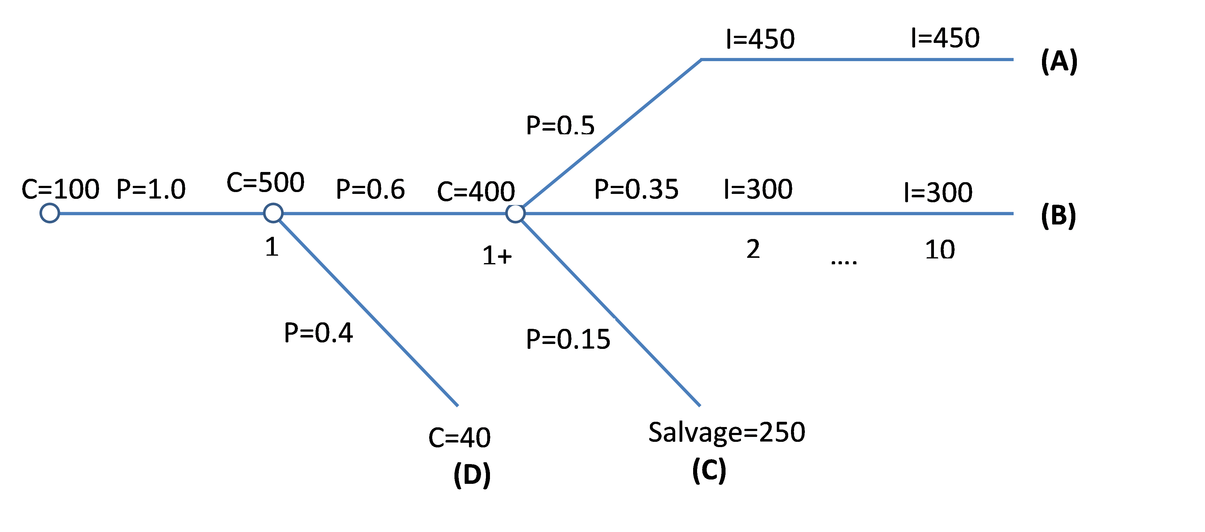
So, there are four stations:
Situation A: Successful development that yields the income of 450 dollars per year
Situation B: Successful development that yields the income of 300 dollars per year
Situation C: Failure that yields a salvage value of 250 dollars at the end of year two
Situation D: Failure that yields abandonment cost of 40 dollars at the end of year one
Probability of situation A can be calculated as
Probability of situation B can be calculated as
Probability of situation C can be calculated as
Probability of situation D can be calculated as
| Probability | |||||||
| A) |
0.3
|
C=$100 | C=$500+$400 | I=$450 | I=$450 | ... | I=$450 |
| B) |
0.21
|
C=$100 | C=$500+$400 | I=$300 | I=$300 | ... | I=$300 |
| C) |
0.09
|
C=$100 | C=$500+$400 | Salvage=$250 | 0 | ... | 0 |
| D) | 0.4 | C=$100 | C=$500+$40 | 0 | 0 | ... | 0 |
|
|
|||||||
| 0 | 1 | 2 | 3 | ... | 10 | ||
Note that the summation of all properties should equal 1.
Project ENPV is the summation of ENPV for all situations. So, first, we need to calculate ENPV for each situation:
And it can be summarized in Table 6-1 as:
| Probability | Year 1 | Year 2 | Year 3 | Year 4 | ... | Year 5 | ENPV | |
|---|---|---|---|---|---|---|---|---|
| A | 0.3 | -$100 | -$900 | $450 | $450 | ... | $450 | $198.5 |
| B | 0.21 | -$100 | -$900 | $300 | $300 | ... | $300 | $33.1 |
| C | 0.09 | -$100 | -$900 | $250 | 0 | ... | 0 | -$60.9 |
| D | 0.4 | -$100 | -$540 | 0 | 0 | ... | 0 | -$220 |
Project ENPV is slightly less than zero compared to the total project cost of 1 million dollars, therefore, slightly unsatisfactory or breakeven economics are indicated.
Please watch the following video (13:32): Expected Value Analysis, Part 2.
PRESENTER: Let's work on a more complicated example. Let's assume a drilling project.
The lease costs would be $100,000 at time 0. That will be paid for all the cases. Then we will have the $500,000 of drilling costs at year 1. Again, this cost is paid for all the cases.
After we paid these $500,000 of drilling costs, we get to the completion point. At this point, there is 60% probability that well logs are good enough to complete the well, which is going to cost $400,000. And there is a 40% failure that they don't look good enough. And we need to close the wells and pay the abandonment cost and so on.
So in case of the 60% probability, let's call it a success case, we will pay $400,000 more in the same year 1 for completion costs. In this case, we will face three cases. One case with a probability of 50%, we will have a producer well, which is going to produce $450,000 per year of income from year 2 to year 10.
And the second case, we are going to have a 35% probability of a well that is going to generate $300,000 per year from year 2 to year 10. And we will have a 15% probability of that the well completion being unsuccessful. And we will have a salvage value of $250,000 for producing equipment in year 2.
So we can summarize the information here. There will be $100,000 of lease costs for all the cases at the present time. And there will be $500,000 of drilling cost at year 1 for all the cases. And then we'll have a 60% probability of getting to the completion. In this case, we pay another $400,000 in year 1. And if I weight 40% probability if we don't complete the well, we need to pay and order $40,000 of costs at year 1.
So in the case of 60%, we will face three new cases. 50% probability that generates $450,000 from year 2 to year 10. And case two, 35% probability of generating $300,000 from year 2 to year 10. And a 15% probability that we don't end up doing anything, any money, any producing well. And we have just a salvage value of $250,000 in year 2.
So the decision tree is a very helpful graph that can help us separate the possible cases here. So I will explain this in this graph. So we start from the left-hand side, the initial investment for the lease at the present time. We write the cost or income here. And in front of that, we write the probability.
So this probability is 100% because it is the same for all the cases. At year 1, we spend $500,000 for drilling, and then, in this case, we are going to have two branches being deviated from the main branch. One is 60%, let's call it a success here, a 60% probability of success and a 40% probability of failure. In case of failure, we are going to pay $40,000 of closing costs, abandonment costs.
In case of success, 60%, we will face another three cases. In case of success, we will pay another $400,000 of completion costs. This 1 plus is to show that this is the same year as this year. These are happening in the same year. But because these cases deviate from the main branch, we draw another branch for these, to separate these from the main branch.
So 60% of success, we pay $400,000 of completion cost. And we will have three new cases in the after. So there is a 50% chance, there is a 50% probability that we will earn $450,000 from year 2 to year 10. So years are here.
So every value under the same column has the same year dimension. We have 35% of getting $300,000 from year 2 to year 10. And we have a 15% probability that we get only $250,000 of salvage at year 2.
So as we can see here, we have four main cases here. Case A, case B, case C, and case D. So the first step to approach this problem and calculate the expected NPV is to calculate the probability of each case. So in order to calculate the probabilities of each case, we go back to the decision tree.
We start from the right-hand side for each case. For example, for case A. So I start from the right-hand side. For example, case A, I start moving from the right-hand side toward the left.
I have a 50% probability here. And go to the main branch. I have a 60% probability here. And I have a 100% probability here. So I will multiply.
I start moving from the right-hand side along each branch to the left, and I multiply the probabilities that I see on the way. So here, I have a 50%, and 60% probability, and a 100%. So I will multiply 50% multiply 60% probability and 100% which has no effect. So the probability of A is 50% multiplied 60%.
B, the probability of case B is 35%, multiply 60%. And multiply this 100%, which has no effect. Case C, probability of 15%, multiply 60%. And case D, the probability of 40% multiply 1, which is going to be 40%. So I calculate the probabilities for case A, case B, case C, and case D.
In the second step, I draw the timeline and I separate the cases from each other. In the first row I write the probabilities. Case A, there is a $100,000 lease cost at the present time. Drilling costs at year 1, plus $400,000 of completion costs.
You remember this was in case the well logs look good. So this $400,000 happens in the same year. And case A is going to generate $450,000 from year 2 to year 10.
Case B, $100,000 of lease costs, plus $500,000 of drilling, plus $400,000 of completion costs. This was happening in year 1. The lease cost is at year 0. And the income from year 2 to year 10.
Case 3. Case 3, the lease cost, the drilling costs, and the completion costs are $400,000 in year 1. And I'm going to have just the salvage of $250,000 in year 2. And the income for other years is going to be 0.
So in case D, which I call it failure case. I pay the lease cost at the present time. I pay the drilling cost in year 1. But the well logs are not looking good enough to pay the completion costs. So I will just close the well and pay the abandonment cost of $40,000.
So now that I have this table calculating the expected NPV. For each case, I calculate the NPV and I multiply that by the probability. And I make a summation over all that.
So here, you can see this is the equation for case A to calculate the NPV. This is the lease cost at the present time. It doesn't need to be discounted.
This is the summation of $500,000 of drilling cost, plus $400,000 of the completion costs. And the $450,000 of income from year 2 to year 10, which they are 9 equal series of income payments. And I need to discount this for one year because they start from year 2.
And the NPV for case B, case C, and case D. Please note that the salvage is happening at year 2 for case C, so I need to discuss that for two years. And I write the NPV for each case in the last column. I multiplied probability by the NPV for each case. And I wrote that too in this column.
And the summation of all these values here is going to give me the expected NPV for this project. And as you can see here, it is going to be about minus $50,000. And the conclusion would be because the expected NPV is slightly negative, is slightly less than 0. We can conclude that this project is not very economically satisfactory.
Credit: Farid Tayari
Italicized sections are from Stermole, F.J., Stermole, J.M. (2014) Economic Evaluation and Investment Decision Methods, 14 edition. Lakewood, Colorado: Investment Evaluations Co.
Risk due to Natural Disaster
One method used to analyze the uncertainty and risk involved in natural disaster decision makings is to choose the best alternative base on the lowest expected cost. In the following example, you can practice this method.
Example 6-7:
A company is planning to build a new plant. The plant requires water for its production process and needs to be built near a river. But the location has the probability of being flooded and building levees around the plant is necessary to protect the facility. There are four possible sizes of levee that have different costs, maintenance, and level of protection, as displayed in following table. Calculate the expected annualized cost for each levee, considering minimum ROR of 12% and 18 years project life. Then explain which levee has the lowest expected annualized cost for the company.
| Levee size | Levee Cost | Probability that levee fails | Expected Damage | Annual maintenance |
|---|---|---|---|---|
| 1 | $150,000 | 0.25 | $100,000 | $3,000 |
| 2 | $180,000 | 0.15 | $130,000 | $4,500 |
| 3 | $200,000 | 0.08 | $140,000 | $5,000 |
| 4 | $220,000 | 0.04 | $180,000 | $7,000 |
Probability of levee failure: Probability of a flood exceeding levee size during the year
Expected Damage: Expected damage if flood exceeds levee size
In order to calculate expected annualized cost for each levee size, we need to convert all the costs into annual base. Then:
From Table 1-12, equivalent annualized levee cost can be calculated as:
Expected damage per year is the multiplication of Probability of levee fails by Expected Damage
Expected annualized cost for different sizes of levee can be calculated as:
| Levee size | Annual Levee Cost | Expected damage per year | Annual maintenance | Expected annual cost |
|---|---|---|---|---|
| 1 | $20690.59 | $25,000 | $3000 | $48,690.59 |
| 2 | $24828.72 | $19,500 | $4500 | $48,828.72 |
| 3 | $27587.46 | $11,200 | $5000 | $43,787.46 |
| 4 | $30346.21 | $7,200 | $7000 | $44,546.21 |
Results show that the third levee has the lowest expected annualized cost; therefore, it is the best alternative.
Summary and Final Tasks
Summary
Sensitivity analysis is a means of identifying those critical variables that if changed, could considerably impact profitability measures such as rate of return or net present value. Risk analysis identifies the likelihood of project failure and the subsequent cost to the investor.
In this lesson, sensitivity analyses for NPV, ROR, project life, and annual payments are practiced. Expected NPV and ROR are also explained to help analyze the effects of risk and uncertainty on the project economics.
Reminder - Complete all of the Lesson 6 tasks!
You have reached the end of Lesson 6! Double-check the to-do list on the Lesson 6 Overview page [37] to make sure you have completed all of the activities listed there before you begin Lesson 7.
Lesson 7: Depreciation and After-Tax Cash Flow
Introduction
Overview
In this lesson, we focus on depreciation, depreciation methods, and After-Tax Cash Flow. An investor is allowed to utilize these methods to recover some types of capital cost. This lesson will explain how these techniques can be used to calculate the taxable income and income tax. To calculate the income tax, taxable income needs to be determined properly.
Learning Objectives
At the successful completion of this lesson, students should:
- understand how Before-Tax Cash Flow and After-Tax Cash Flow are calculated;
- be able to apply Straight Line, Declining Balance, and Declining Balance Switching to Straight Line methods for depreciation calculations; and
- be familiar with modified accelerated cost recovery system (MACRS), Depletion, and Amortization.
What is due for Lesson 7?
This lesson will take us one week to complete. Please refer to the Course Syllabus for specific time frames and due dates. Specific directions for the assignment below can be found within this lesson.
| Reading | Read Chapter 7 of the textbook and following pages in this lesson in the website. |
|---|---|
| Assignment | None. |
Questions?
If you have any questions, please post them to our discussion forum, located under the Modules tab in Canvas. I will check that discussion forum daily to respond. While you are there, feel free to post your own responses if you, too, are able to help out a classmate.
After Tax Cash Flow
After revenue and costs are determined, taxable income and income tax need to be calculated. Tax calculations can be very complicated, but here we just address the basics. Usually, in a specified time period, total costs deducted from total revenue gives the taxable income. Before-Tax and After-Tax Cash Flow can be calculated as:
Revenue
− Operating Costs
− Capital Cost
————————————————
Before-Tax Cash Flow (BTCF)
− Income Tax
————————————————
After-Tax Cash Flow (ATCF)
Operating and Capital Costs deducted from Revenue gives the Before-Tax Cash Flow. And After-Tax Cash Flow equals Before-Tax Cash Flow minus Income Tax.
Example 7-1:
Assume a project that has the estimated gross revenue of $28,000 dollars, operating cost of $12,000, and capital cost of $10,000 next year with the income tax of $1,500. Then, next year After-Tax Cash flow can be calculated as:
From a tax view point, there are two types of investments. According to US tax law, for the purpose of tax calculations, an investor is allowed to recover some specified types of investments, meaning that the investor can take some amounts of money from the generated revenue as tax deductions. Types of property that may be recovered over their useful lifetime are including (but not limited to) building, machinery, equipment, and trucks. Simply, most of the property types that lose their value over the time (have zero or low salvage value) may be allowed to be recovered. On the other side, there are investments that can’t be deducted from income for tax purposes. Investing in a bank account or buying land are the examples of this type.
Example 7-2:
Assume an investor deposits $100,000 in a bank account for 10 years with annual interest of 16% and will take the $100,000 in the end of 10th year. Calculate Before-Tax Cash Flow and After-Tax Cash Flow in this investment considering the income tax of 25%.
The annual income will be .
Since tax deduction is not allowed for investments such as bank account and bond, the annual revenue is fully taxable.
| Year | 0 | 1 | 2 | 3 | ... | 9 | 10 |
|
|
|||||||
| Revenue | $16,000 | $16,000 | $16,000 | ... | $16,000 | $16,000 | |
| - Cost | -$100,000 | ||||||
| + Salvage | $100,000 | ||||||
|
|
|||||||
| BTCF | -$100,000 | $16,000 | $16,000 | $16,000 | ... | $16,000 | $116,000 |
In order to determine After-Tax Cash Flow, we need to determine the taxable income and deduct the tax from Before-Tax Cash Flow.
| Year | 0 | 1 | 2 | 3 | ... | 9 | 10 |
|
|
|||||||
| Revenue | $16,000 | $16,000 | $16,000 | ... | $16,000 | $16,000 | |
|
|
|||||||
| Taxable Income | $16,000 | $16,000 | $16,000 | ... | $16,000 | $16,000 | |
| - Income Tax of 25% | -$4,000 | -$4,000 | -$4,000 | ... | -$4,000 | -$4,000 | |
|
|
|||||||
| Net Income | $12,000 | $12,000 | $12,000 | ... | $12,000 | $12,000 | |
| - Cost | -$100,000 | ||||||
| + Salvage | $100,000 | ||||||
|
|
|||||||
| ATCF | -$100,000 | $2,000 | $12,000 | $12,000 | ... | $12,000 | $112,000 |
By trial and error, the ROR=12% is calculated for this After-Tax Cash Flow.
Example 7-3:
Now, assume the investor pays 100,000 dollars for a machine at time zero, and the machine can start producing goods and generating annual revenue of $38,000 with operating cost of $12,000 from first to 10th year, and the salvage value will be zero with income tax of 25%.
The Before-Tax Cash Flow here can be determined as:
| Year | 0 | 1 | 2 | 3 | ... | 9 | 10 |
|
|
|||||||
| Revenue | $38,000 | $38,000 | $38,000 | ... | $38,000 | $38,000 | |
| - Operating cost | -$12,000 | -$12,000 | -$12,000 | ... | -$12,000 | -$12,000 | |
| - Capital cost | -$100,000 | ||||||
|
|
|||||||
| BTCF | -$100,000 | $26,000 | $26,000 | $26,000 | ... | $26,000 | $26,000 |
By trial and error, ROR=22.6% for Before-Tax Cash Flow.
In this hypothetical case, the investor is allowed by tax law to recover the out of pocket cash “capital cost” and gradually deduct it from taxable income. One way to calculate the taxable income for each year is to distribute the capital cost of $100,000 equally over the allowable depreciation life time of 10 years. And After-Tax Cash Flow will be determined as:
| Year | 0 | 1 | 2 | 3 | ... | 9 | 10 |
|
|
|||||||
| Revenue | $38,000 | $38,000 | $38,000 | ... | $38,000 | $38,000 | |
| - Operating cost | -$12,000 | -$12,000 | -$12,000 | ... | -$12,000 | -$12,000 | |
| - non-cash capital cost deduction | -$10,000 | -$10,000 | -$10,000 | ... | -$10,000 | -$10,000 | |
|
|
|||||||
| Taxable income | $16,000 | $16,000 | $16,000 | ... | $16,000 | $16,000 | |
| - Income tax | $4,000 | $4,000 | $4,000 | ... | $4,000 | $4,000 | |
|
|
|||||||
| Net Income | $12,000 | $12,000 | $12,000 | ... | $12,000 | $12,000 | |
| + non-cash capital cost | $10,000 | $10,000 | $10,000 | ... | $10,000 | $10,000 | |
| - Capital cost | -$100,000 | ||||||
|
|
|||||||
| ATCF | -$100,000 | $22,000 | $22,000 | $22,000 | ... | $22,000 | $22,000 |
This way, the taxable income for each year would be 16,000 dollars, which gives the tax of . Note that, in reality, no annual cash is transferred and the annual sum of $10,000 (non-cash capital cost deduction) is applied just for the purpose of tax calculations. This annual sum is called non-cash capital cost to adjust and recover the the capital cost of $100,000 at time zero. And when tax is calculated, $10,000 has to be returned to cash flow to give the After-Tax Cash Flow.
ROR for After-Tax Cash Flow is 17.7%.
Applying tax deductions to recover the investment causes lower taxable incomes and consequently lower taxes and can only be used for specified types of properties. Investments that are allowed to be recovered by tax law are divided into two categories.
1)Investments that can be expensed: These investments are allowed to be deducted from revenue in full amount in the year of occurrence for tax calculation.
2) Capital costs: These investments are allowed to be deducted gradually (cost needs to be distributed over more than one year) from the revenue for tax calculation.
Depreciation, depletion, and amortization are methods that can be utilized to calculate the distribution of capital costs deductions over the time.
Acquisition costs and lease bonus costs paid for mineral rights for natural resources such as oil and gas are examples of investment property costs that may be recovered by depletion. Numerous other business costs such as the cost of acquiring a business lease, research and development costs such as expenses, trademark expenses, and pollution control equipment costs may be recovered by amortization. Depreciation, depletion, and amortization all achieve essentially the same thing—recovery of the cost or other basis of investments in before-tax dollars through allowable tax deductions over a specified period of time or over the useful life of the investment. If depreciable property is sold, all or a portion of any extra depreciation claimed in prior years may have to be recaptured as taxable income. These methods will be explained in this lesson.
Please watch the following video (4:34): After Tax Cash Flow.
PRESENTER: In this video and following videos, I will explain how to calculate tax deductions and after tax cash flow. Tax law allows the investors to recover some unspecified types of their investment through tax deductions, meaning that the investor can take some amount of money from generated revenue as tax deductions. Types of property that may be covered over their useful life are including but not limited to building, machinery, equipment, and trucks.
If the property doesn't lose its value, it cannot be recovered through tax deductions. A good example of that is bank accounts or land. If you buy land, it is assumed that the land value is not going to be lower after a couple of years. So you're not allowed to recover the amount of money that you paid for the land through tax deductions.
So there are two main categories of investments that can be-- that are allowed to be recovered through tax deductions. The first category is called investments that can be expensed. Expensed means they can be recovered in full amount in the year that they happen. An investor can deduct that expense, that investment, in full amount, from the revenue in the year that investment has occurred.
The other type of investments are the ones that can be capitalized. Capitalized means they can be deducted over more than one year as tax deductions. So the difference between investments that can be expensed from the investments that can be capitalized is just the time.
Here, we can see business costs that can be expensed. They can be deducted in full amount in the year that they happen-- operating costs, research and experimental costs, mining, exploration costs, mining development costs, petroleum intangible drilling costs, or IDC. Depreciation, depletion, and amortization are methods to capitalize the business costs. And essentially, they do the same thing.
But they are applicable to different categories of costs-- for example, acquisition costs and lease bonus costs or paid for mineral rights or natural resources. They can be recovered by depletion, and costs such as acquiring a business lease or trademark expenses, they can be recovered by amortization. So it is obvious that the faster investors recover their expenses, it's better for them. It is going to have positive economic effect on the project. For example, if there is no limitation in recovering the investments, investors would prefer to recover all their costs, all the investment, in full amount in the year that they are paying that because the earlier you get your money back, it has higher value than when you get it in a later future.
In general, After-Tax Cash Flow requires the following calculations:
Revenue
- Operating Costs
- Depreciation
- Depletion
- Amortization
- Write-offs
————————————————
Taxable Income
- Income Tax
————————————————
Net Income
+ Depreciation
+ Depletion
+ Amortization
+ Write-offs
- Capital Expenditures
————————————————
After-Tax Cash Flow (ATCF)
Where, Depreciation, Depletion, Amortization, and Write-offs are called Non-cash capital cost deductions. ATCF can be written in form of equation as:
Or
As explained in Example 7-2 and 7-3, depending on the characteristics of investment, Before-Tax Cash Flow and After-Tax Cash Flow calculations might be different and may give different economic results.
Italicized sections are from Stermole, F.J., Stermole, J.M. (2014) Economic Evaluation and Investment Decision Methods, 14th edition. Lakewood, Colorado: Investment Evaluations Co.
Business Costs that May Be Expensed
As explained on the previous page, there are two types of investments that are allowed to be recovered and deducted from revenue for tax calculation. These two types include: the investments that can be expensed (deducted in full amount on the year occurred) and capital costs that have to be deducted (“capitalized”) over more than one year.
It’s obvious that the faster an investor can deduct the recoverable investments from the revenue, the better economic benefits will be for the project. For example, if there is no limitation, the investor is better off if deducting all the investments in full amount in the year of occurrence and paying lower tax in early years than later years. (We learned in this course that money is worth more on closer future). But tax law doesn’t allow all the investments to be expensed, and there are strict regulations for different types of investments.
Operating Costs
Operating costs that may be expensed include costs for direct labor, indirect labor, materials, parts, and supplies used for product produced and sold. Only costs associated with product actually sold may be deducted. Some other common costs in the operating expense category include utilities, freight and containers, borrowed money interest paid, royalties, severance taxes, sales taxes, ad valorem taxes, and certain excise taxes. Note that costs such as spare parts inventory, accounts receivable, required cash on hand, etc., are not deductible for tax purposes until such items are actually used up or sold. These costs are called working capital.
Research and Experimental Costs
Research and experimental costs including labor, supplies, etc., are considered to be the equivalent of operating costs and may be expensed in the year incurred.
Mining Exploration Costs
Mining exploration costs are expenditures required to delineate the extent and quality of an ore body and may include core drilling, assaying, engineering fees, geological fees, exploratory shafts, pits, drifts, etc. Exploration costs may be either capitalized into the cost depletion basis or expensed in the full amount in the year incurred by individual taxpayers.
Mining Development Costs
Mining development costs are defined as expenditures incurred after the determination has been made that an ore body is economically viable and the decision has been made to develop the property. Development costs may include exploration type costs after the decision has been made to develop a mine. Mining development costs typically include costs for overburden stripping, underground shafts, drifts, tunnels, raises, audits, etc. Development expenditures end when a mine reaches a level of full production. Then, costs that previously were mine development costs are treated as operating expenses from the time forward.
Petroleum Intangible Drilling Costs (IDC's)
Petroleum Intangible Drilling Costs (IDC's) are defined as the cost of drilling oil and gas wells to the point of completion and may include:
- Costs of agreements with operators and drilling contractors
- Survey and seismic work related to location of a well
- Road cost to well location to be used during drilling
- Dirt work on location for pit, etc.
- Rig transportation and set-up costs
- Drilling costs including fuel, water, drilling mud, etc.
- Costs of technical services including engineering, geologists, logging, and drill stem test services
- Cost of swabbing, fracturing, and acidizing
- Cementing of surface casing and main casing (not the cost of casing)
- Reclamation of well site
Similar to mining development costs, intangible drilling costs may either be capitalized into the cost depletion basis or expensed in full amount in the year incurred.
Italicized sections are from Stermole, F.J., Stermole, J.M. (2014) Economic Evaluation and Investment Decision Methods, 14th edition. Lakewood, Colorado: Investment Evaluations Co.
Business Costs that May Be Capitalized
Depreciation and Depreciation Methods
As explained before, depreciation is a method to capitalize and recover business costs over a specified period of time or over the useful life of the investment.
The term depreciation [38] usually refers to the process of losing value over the time for a property, like wear and tear. When a machine is purchased to produce and generate income, it won’t be as good when it becomes older. It happens because the machine gets exhausted or production becomes obsolete. Therefore the machine loses its value over time and can’t be sold for high value. Tax law allows the company to deduct the depreciated value of the asset from the generated income. There are permitted methods (will be explained later in this lesson) to calculate the depreciated value, which might be different from how the asset depreciates in reality. For example, the asset might be still functional while it is already fully depreciated in tax calculations. In this text by the term annual depreciation deduction we refer to tax allowance.
A depreciable property:
- must be used (or be ready to be replaced) for producing income;
- must have a determinable lifetime longer than one year;
- must lose its value over time;
- must be used or be ready to be used.
For example, land is an asset that is not permitted for depreciation. More information about depreciation can be found at the Internal Revenue Service (IRS) website [39]. Depreciation is usually applied to the tangible [40] property while amortization is for intangible [41] property.
Depreciation Methods
This section explains four major depreciation methods including:
- Straight Line
- Declining Balance
- Declining Balance Switching to Straight Line
- Modified Accelerated Cost Recovery Systems (MACRS)
Please watch the following video (4:20): After Tax Cash Flow: Expensing Versus Capitalizing Investment Costs.
PRESENTER: As explained in the previous video, tax law allows investors to recover some of their investments through tax deductions. In explaining that, there are two main methods for the investment costs, cost that can be expensed and cost that can be capitalized. And the difference is only time, the cost that can be expensed or the cost that can be deducted in full amount from the income and cost that can be capitalized or the cost that can be deducted gradually over time, more than one year from the revenue income.
So depreciation is one of the methods of business cost that can be capitalized. They have to be deducted from revenue or income over the years, more than one year, gradually. The depreciation means the process of losing the value over time for property, like wear and tear.
For example, when an investor buys a machine for producing and generating income, after a couple of years the machine gets older. It would require maintenance and repair more frequently. The quality of the units that it produces becomes lower. The technology becomes obsolete. And the machine loses its value over time and it cannot be sold for a very high value.
So the tax law allows the company, the investor, to deduct the depreciated value of the asset from the generated income. So tax law allows some standard methods to apply the depreciation and using the tax deduction to recover the costs of the depreciated property or machinery or building.
These are standard accounting methods. And they might be different from the actual physical depreciation of the property. So the property might still be functional and working while it is fully depreciated. And the cost of it is recovered through tax deductions. So these are different.
So depreciation method is allowed to be used for property that has these four characteristics. The property must be used or be ready to be replaced for producing income. The property must have a determinable lifetime longer than one year.
The property must lose its value over that time. For example, land, it is assumed that land doesn't lose its value over time. So we cannot use depreciation for recovering land costs. And, also, the property must be used or be ready to be used.
There are four major depreciation methods; a straight line method, declining balance, declining balance switching to straight line [AUDIO OUT], and modified accelerated cost recovery system, or MACRS, that I will explain in the following videos.
1. Straight Line Depreciation
This method is the simplest way of calculating the depreciation. In this method, depreciation is constant and equally distributed over the allowable life time of the property as:
The biggest problem in this method is straight line depreciation is very slow and capital cost is recovered slowly. The faster costs are recovered the lower tax is paid in early years and it enhances the economics of the project.
Straight line depreciation is the method that used to calculate the non-cash capital cost deduction in Example 7-3.
Example 7-4:
Following the Example 7-3, assume allowable depreciation life time is 5 years, starting from year 1. Also assume the investor buys a piece of land for $25000 at time zero that can be sold at year 10 for $35,000.
Note that investment for land is not depreciable. The land resale value of $35,000 should be added to the income of 10th year. But the initial value of land is deductible as “Write-off”. Because, just the profit ($35,000 - $25,000 = $10,000) made on selling the land is taxable.
After-Tax Cash Flow will be determined as:
| Year | 0 | 1 | 2 | 3 | 4 | 5 | 6 | 7 | 8 | 9 | 10 |
|
|
|||||||||||
| Revenue | $38,000 | $38,000 | $38,000 | $38,000 | $38,000 | $38,000 | $38,000 | $38,000 | $38,000 | $38,000 | |
| +Land resale | $35,000 | ||||||||||
| - Operating cost | -$12,000 | -$12,000 | -$12,000 | -$12,000 | -$12,000 | -$12,000 | -$12,000 | -$12,000 | -$12,000 | -$12,000 | |
| - Depreciation | -$20,000 | -$20,000 | -$20,000 | -$20,000 | -$20,000 | ||||||
| - Write-off | -$25,000 | ||||||||||
|
|
|||||||||||
| Taxable income | $6,000 | $6,000 | $6,000 | $6,000 | $6,000 | $26,000 | $26,000 | $26,000 | $26,000 | $36,000 | |
| - Income tax | $1,500 | $1,500 | $1,500 | $1,500 | $1,500 | $6,500 | $6,500 | $6,500 | $6,500 | $9000 | |
|
|
|||||||||||
| Net Income | $4,500 | $4,500 | $4,500 | $4,500 | $4,500 | $19,500 | $19,500 | $19,500 | $19,500 | $27,000 | |
| + Depreciation | $20,000 | $20,000 | $20,000 | $20,000 | $$20,000 | ||||||
| + Write-off | $25,000 | ||||||||||
| - Capital cost | -$100,000 | ||||||||||
| - Land | -$25,000 | ||||||||||
|
|
|||||||||||
| ATCF | -$125,000 | $24,500 | $24,500 | $24,500 | $24,500 | $24,500 | $19,500 | $19,500 | $19,500 | $19,500 | $52,000 |
ROR for After-Tax Cash Flow will be 14.5%.
Half-year convention
Under half-year convention properties are assumed to be placed in service in the middle of the year. Consequently, half of the first year normal depreciation has to be applied to the year that the property is placed in service. For example, if half-year convention is applied to the first year in example 7-4 to calculate the depreciation using Straight Line method, then the calculated depreciation would be:
| Year | Half-year convention straight line Depreciation |
|---|---|
| 1 | |
| 2 | |
| 3 | |
| 4 | |
| 5 | |
| 6 | |
| Total | $100,000 |
Note that because we applied half-year convention to the strait line depreciation method we considered half of the first year normal depreciation for year 1, thus we needed to add the rest (other half) to the year 6; consequently there will be 6 years of depreciation periods.
Please watch the following video (23:32): Straight Line Depreciation Method.
PRESENTER: In previous videos, I explained investment costs that can be capitalized, and I briefly explained the depreciation methods. So as I explained, there are four major depreciation methods. First one is a straight line that I'm going to explain in this video.
Second one is declining balance. The third one is declining balance switching to the straight line. And the last one is modified accelerated cost recovery system, or MACRS, that I will explain in the next videos.
Straight line depreciation is the simplest method in calculating depreciation. In this method, we uniformly distribute depreciation over the years of allowable lifetime of the property. So the equation is the cost of the asset-- the actual cost that you pay for the asset-- minus the salvage value, if there is any salvage value, divided by the number of years that we want to depreciate that property over those years.
So this method is very simple. But the problem is, it is very slow, as we explained before. The investor would like to recover the capital cost as soon as possible. The more years, the longer it takes, to recover the money. So they get the same amount of money every single year. They get the same amount of depreciation every single year.
So and we know that the faster costs are recovered, the lower taxes paid in the early years. And it is going to enhance the economics of the project. The earlier the investor gets the tax deduction, it improves the economics of the project.
So let's assume an investor pays $100,000 for a machine, that this investment can be depreciated using the straight line depreciation over the five years, from year one to year five. The machine will start producing and generating revenue from year one to year 10, with a revenue off $38,000, and operating costs of $12,000. The salvage value is going to be zero.
And also, the investor has to buy land, for cost of $24,000, at time, zero. But because land doesn't lose its value over time, we assume the land resale value, in the end of the year 10, is going to be $35,000. So we consider the income tax of 25%, and we want to calculate after-tax cash flow.
First, we need to calculate the depreciation. The capital cost for the machinery was $100,000. And it can be depreciated over five years. And with a straight line depreciation, we have five years of uniform distribution. And the salvage value is zero.
So the depreciation for each year is going to be calculated as $100,000, divided by 5 years. And we are going to have $20,000 of depreciation for each year, from year one to year five, that can be deducted from revenue as tax deductions. Here, please note that the land is not depreciable.
So the land is purchased for $25,000, at present time, and it is going to be sold at $35,000, in the end of the year 10. So the investor is going to make $10,000, which is the difference between the purchasing cost and the resale cost, resale price. The investor has to pay tax on the $10,000 of profit that is going to be earned at year 10.
And now, the second step is, we draw this table. We start with revenue, whatever generates income. The first is, we have $38,000 of revenue created by the machine. Then, we are going to have-- we are going to sell the land at year 10. So we are going to have $35,000 of cash, after we sell the land in year 10, but we can see, we-- I'll show you later, in a bit, that just $10,000 of debt has to be taxed.
So then we start adding costs-- the operating cost of $12,000 from year one to year 10. Then we add depreciation. So the depreciation should be-- we should enter depreciation with a negative sign. And we can-- it has to be deducted from revenue as tax deduction, before calculating the tax.
So we have five years of depreciation, and it is uniformly distributed. Every year is $20,000 we deduct from revenue, from year one to year five. And I had this item called write-off, because we are going to sell the land at $35,000. We are going to have the revenue of $35,000 at the year 10. But we pay $25,000 for land, at the present time.
So this profit that we made on the land is taxable, and not the actual capital cost that we pay for the land. So we write these land write-off, of minus $25,000, to adjust these income that-- saying that, OK, just the $10,000 of the money that we made on the land is taxable.
Then, we calculate the taxable income, which is the summation over each column. And the income tax of 25%, which is 25% of taxable income. And we calculate that for every column.
And what we have is net income, which is the summation of these two rows. If we enter the tax with a negative sign, this is going to be with the summation. If we don't enter the tax with negative sign, then it will be the difference between these two. So taxable income minus income tax is going to give us net income.
And we calculate that for every single year, from year zero-- from present time-- to year 10. Here, because we don't have any income or any cost, we don't have any net income at year zero, but later on we will see that we are going to have all our capital costs and land costs here at year zero.
So then, we start adding back whatever we deducted here, for tax deductions. So we deducted the depreciation. We calculated the tax. And then, we add that back again. So negative sign here, and then you add that with the positive sign. These are exactly the same.
The next thing is land write-off. We add back the land write-off of $25,000, and then we enter the capital cost. So we had-- the investor invested $100,000 at present time, for buying the machinery, and the land, which was purchased for $25,000. Please note that for the write-off, we have a minus number here, before calculating the tax, and we add that back again. And here, we have the resale value of the land.
And we calculate the after-tax cash flow, by making a summation over each column-- net income plus depreciation plus write-off minus capital cost minus land. And this is going to be our after-tax cash flow.
So let's work on this example in a spreadsheet, and see how we can use a spreadsheet-- Microsoft Excel or any other spreadsheet-- to approach these problems. So first, I'm going to write the year. I start from year zero. There are 10 years. The lifetime of the project is going to be 10 years, so I will have 10 years of project lifetime, here.
Then, the first thing that I have to do, I start with the revenue, with the items that have the nature of making money, creating some revenue. So revenue that is generated by the machine-- machine comes to production at year one, and produces from year one to year 10, and generates $38,000. One important point, here, is you have to have all your input data in a separate section, and you have to refer to those cells that you need.
And very good feature about the spreadsheet is if you update some inputs, it is going to automatically update your output, as well. So instead of writing $38,000, from here, here, here, and to year 10, I will just refer that to the input data that I have, here. So I write equals sign and this one.
And because-- so it writes the $38,000, here, but because I want to apply this to the other 10 years, I will put a dollar sign before there, the column number. Then, when I apply this, it keeps the-- the year keeps the same cell for all the years. So there is no revenue at year zero, so I skipped that. I left that blank.
Then, I'm going to have land resale value. Excel is confusing this as an equation, so I can just delete that, because I start with a positive sign. So I can just put the sign, and it will accept it as just the text. So the land resale is going to be $35,000, at year 10.
Then, I will add the operating cost with the negative sign. Operating cost-- so I'm going to add the operating cost from year one to year 10. So negative sign-- I read the operating cost from here. I fixed the column number, and then apply that from year one to year 10.
Then I'm going to have the depreciation with the negative sign. Depreciation-- I can actually calculate the depreciation number here, and read that from-- refer to that cell. I can say year depreciation, year zero, year zero, one, two, three, four, five.
And the depreciation equals the capital cost divided by 5 years of depreciation. I fixed this one. And this is a straight line, so I'm going to have $20,000 per year from year one to year five. Sorry, I don't have depreciation at year zero. So I'm going to enter depreciation with a negative sign, here. Year one, year two, three, four, and five.
And I will add the land write-off with the negative sign. Then I will draw a line, here, because I want to calculate the taxable income.
So taxable income, I have to make a summation over each column. There is nothing, at present time. So summation of all these values, at year one, and I apply that to year 10. I calculate the tax with the negative sign. So that is going to be 25% of this amount, 25% of taxable income. And I apply this to year 10.
Again, I draw a line here, and I calculate net income, which is going to be-- I could have the tax with the positive sign, and then deduct these two, or I could have the tax with the negative sign, and just simply make a summation, here. So I will enter the tax with the negative sign, and make a summation here, and calculate the net income.
After we calculate the net income, we have to add back whatever we had, here, as the tax deductions. So we had this depreciation, and we had land write-off. So we add them back with the positive sign.
And it is exactly the same as here. So I will just multiply this number with the negative sign. This is for five years. I apply that for five years. Then the land write-off with the positive sign, which is going to be at year 10.
And we are going to have the capital cost with a negative sign. So the capital cost-- what was happening at the present time. So negative, and I read it from here. And we paid for land, at present time.
So land-- again, I draw a line here, because I want to calculate the after-tax cash flow. And after-tax cash flow is simply the summation between these two lines. So now I have the after-tax cash flow calculated in this row. OK.
There is a version of straight line depreciation method that is called half-year convention. So in this method, it's exactly the same as the straight line depreciation, but we move everything for six months forward. So the intuition behind that is, it takes a while, maybe, for the machinery to come to production.
So we start in the middle of the year, not in the beginning of the year. So we move everything for six months forward. So we take six months from the first year, and we add an extra year to the end, with only six months.
So for example, if you want to calculate the same depreciation for the same example-- investing $100,000 into machinery-- using half-year convention, we just move everything for half a year to forward. For the straight line depreciation, for each year we had one-fifth, because we had 5 years of depreciation, and the salvage value was zero. So $100,000 divided by 5. For each year, we are going to have $20,000 of depreciation from year one to year 20.
But if we use the half-year conventional straight line depreciation, for the first year, we are going to have half of the depreciation. So we are going to have half of the $20,000, which is $10,000, which means that we have just six months in the year one, and we add that to the last year. So we are going to have one extra year in the end. And we are going to have, add this six months to these-- we are going to have this extra year with only six months.
Again, the summation here is exactly $100,000, and the summation here is exactly $100,000. Please note that with half-year convention, we have one more year, here. So if you want to apply this half-year convention straight line depreciation to our spreadsheet, we come back here. We are going to have one more extra year, here.
So we divide this by 2, which we are going to have $10,000 here. And we are going to have this $100,000 divided by 5, divided by 2, here. Again, if I calculate the summation here, it should be exactly same as $100,000.
We go back here to this depreciation. We can see it is updated from here, but because we are going to have one more year, I need to apply this to one more year. And here, I'm going to apply, add that to, one more year, here. So we have six months less, here, but we have one more year, here, with extra six months.
2. Declining Balance Depreciation
This method is also called “exponential depreciation” and calculates the depreciation based on constant rate (instead of constant amount as the case for straight line depreciation). This method is not allowed in United States, but in some other countries companies can use it. In this method, a constant declining rate is multiplied by Adjusted Basis to calculate each year’s depreciation. And the Adjusted Basis equals residual book value of the asset (cost - cumulative depreciation previously taken).
While for any depreciation method,
For example, if the declining rate is 0.25 and the asset is purchased at $100.
Some governments announce the declining balance rate as a percentage that needs to be multiplied by 1/n (n is the depreciation life) to give the declining rate. For example, if an asset has the depreciation life of 5 years and the government announces 150% declining balance rate, then the declining curve would be 1.5/5= 0.3.
Example 7-5:
Calculate the depreciation in Example 7-3, assuming declining balance depreciation method, declining balance rate of 150%, and depreciation life of 5 years.
Since depreciation life is considered 5 years, then declining rate equals 150%/5 = 0.3 so depreciation can be calculated as:
| Year | Adjusted Basis | Declining Balance Depreciation |
|---|---|---|
| 1 | $100,000 | |
| 2 | ||
| 3 | ||
| 4 | ||
| 5 | ||
| Total | 83,193 | |
As you can see, the last row shows that total of $83,193 is less than the capital spent on the property ($100,000). Thus in this method asset will not be fully depreciated.
Please watch the following video (15:34): Declining Balance Depreciation Method.
PRESENTER: In the previous videos, I explained that investors can recover some types of their investments using tax deductions. Tax deductions are categorized in two main groups-- investment costs that can be expensed and investment costs that can be capitalized. Time is the only difference between these two categories.
If a cost can be deducted from revenue in full amount as tax deduction in the year that it has happened, the cost is expensed. Costs such as operating costs can be in this category. If a cost has to be deducted from revenue as tax deduction in more than one year, it is called capitalized, such as money that is paid for machinery, building, and so on. Things that generally lose their value over time are allowed to be in this category.
Then in the previous video, I explained the depreciation as one method that we can capitalize on investment cost. And as I explained in the previous video, there are four major methods of depreciation. I explained the straight line and the straight line half year convention in the previous video. And in this video, I'm going to describe the second method, which is declining balance depreciation method.
Declining balance depreciation is also called exponential depreciation. This method is not used and allowed in the United States. But the modified versions of this method are widely used. So we're going to learn this method first, because the other methods are based on the declining balance depreciation. So declining balance depreciation considers a constant depreciation rate. In the straight line, the depreciation was constant.
Here, for the declining balance, the depreciation rate is constant over the years. So in this method, we multiply the constant declining rate by the adjusted basis. Let's work on this example to see how the declining balance depreciation works. In this example, we assume the declining rate is 25%, and the asset is purchased at $100 with no salvage value.
So the residual book value for year one includes $100 minus a salvage value of zero. So we are going to have $100 of residual book value for year one. In order to calculate the depreciation for year one, we multiply the rate of 25% by the $100. And we're going to get $25 of depreciation for year one.
For the second year, we deducted the depreciation rate from $100. And we are going to have the adjusted basis of $75 for year two. We multiply that by 25%. And we get $18.75 of depreciation for year two.
For year three, we need to calculate the adjusted basis first. In order to calculate the adjusted basis, we deduct the depreciation of the previous year from the adjusted basis of the previous year to calculate the adjusted basis for year three.
So $75 is the adjusted basis in year two. And the $18.75 is the depreciation at year two. And it is going to be equal to $56.25. We multiply that by the declining rate, which is constant over the rate over the years. And we are going to have $14.06 of depreciation for year three.
For the year four, we follow the same method-- adjusted basis of previous year minus the depreciation of the previous year. And it is going to give us $42.19 of adjusted basis for year four. We multiply that by the declining rate depreciation rate, and we get $10.55 for depreciation for year four.
So here we calculated the depreciation just for four years. Some countries announce the declining balance rate as a percentage that has to be divided by the number of years, by the depreciation life, n, to calculate the declining rate per year. For example, if the asset can be depreciated over the lifetime of five years, and the government announced a 150% of declining balance rate, to calculate a declining rate per year, we just need to divide the 150% by the 5.
Let's work on another example. In the previous video, I calculated the depreciation for an asset that was purchased at $100,000 with the salvage value of 0, using the straight line depreciation method. In this example, I'm going to calculate the depreciation using the declining balance method. And I'm going to consider declining balance rate of 150% and depreciation life of five years.
So the first thing that we have to do is we have to calculate the declining rate per year. So we divide the 150% by the five years of the depreciation life. And we are going to get 30% of depreciation rate per year.
So to calculate the depreciation for the first year, we multiply the adjusted basis, which was $100,000, by the declining rate that we have, 30%. And we are going to get $30,000 of depreciation for year one.
For year two, we need to deduct the depreciation of the previous year from the adjusted basis of the previous year, so $100,000 of the adjusted basis at year one minus $30,000-- the depreciation at year one-- equals $70,000. And this is the adjusted basis at year two. We multiply that by the declining balance of 30%. This is the constant rate. And we are going to get $25,000 of depreciation for year two.
For year tree, $49,000 of adjusted basis for year three-- we multiplied that by the declining rate and $14,700 of depreciation for year three. We follow the same method for year four-- adjusted basis of the previous year minus the depreciation of the previous year. It gives us the adjusted basis for year four. We multiply that by the depreciation rate per year. And we calculate the depreciation. And for year five.
So one very important thing here to notice is the cumulative depreciation here-- the summation of all the depreciations from year one to year five-- is less than the depreciable value, which was $100,000. So in this matter, the asset is not fully depreciated. And for the straight line method, for the straight line depreciation method, we fully depreciated the asset.
So we had $20,000 of depreciation at each year. And the summation was $100,000. But in this method, the money that the investor gets is less than the money spent on the asset. But this method is very fast. The investor gets the biggest portion of the money very quickly. As you can see here, almost 50% of the depreciated value is received as tax deduction in the first two years.
So let's work on this example on an Excel spreadsheet and see how we can formulate these kind of examples, these kind of problems, using a spreadsheet. So in this spreadsheet, we can see the previous example that we had half year convention straight line depreciation. So I'm just going to delete these and apply the declining balance rate. So depreciation equals--
So the declining rate per year equals the 150% divided by five years of depreciation [? lifetime. ?] And we are going to have that 30% of depreciation rate or declining rate per year. So here I'm going to use vertical formatting this time-- year adjusted basis here and depreciation. One, two, three, four, five.
So adjusted basis for year one equals $100,000. So the depreciation equals adjusted basis, multiply the declining rate. So we are going to have $30,000 of depreciation for year one.
For year two, in order to calculate the adjusted basis, I need to deduct the depreciation of the previous year from the adjusted basis of the previous year. So adjusted basis equals $100,000 minus depreciation of the previous year. And the depreciation for year two equals the adjusted basis, multiply the declining rate.
For year three, adjusted basis of the previous year minus the depreciation of the previous year. And depreciation equals adjusted basis, multiply the declining rate per year. And we do this for year four and year five.
Again, here very important thing to note is the summation of all these depreciation in the declining balance rate method is less than $100,000. So I calculate this summation.
So we can see the summation is less than the $100,000 of capital cost. And now, I enter these depreciations to the cash flow. So year to the before-tax cash flow. So depreciation for year one equals minus this number. Depreciation for year two equals $21,000 that I calculated, depreciation for year three and so on to year four.
And you can see-- because I have already everything set up, the depreciation is going to be updated after I calculated the net income. They are going to be exactly the same and with a positive sign. And there is nothing here, so we'll just end.
3. Declining Balance Switching to Straight Line
In this method, depreciation is calculated using declining balance for early years and then switches to the straight line method. It is desirable to switch to straight line from declining balance in the year when you will get an equal or larger deduction by switching. This occurs when the straight line rate equals or exceeds the declining balance rate, because when you switch, the remaining basis is depreciated by straight line method over the remaining years of depreciation life.
Example 7-6:
Calculate the depreciation in Example 7-3, applying declining balance depreciation switching to straight line method for declining balance rate of 150% and depreciation life of 10 years.
Depreciation life is considered 10 year, then declining rate equals 150%/10 = 0.15.
Here, it’s more economically desirable to switch to the straight line method after the fourth year, because the annual depreciation will be higher when switching from declining balance to straight line.
| Year | Method | Adjusted Basis | Declining Balance Depreciation |
|---|---|---|---|
| 1 | DB | $100,000 | |
| 2 | DB | ||
| 3 | DB | ||
| 4 | DB | ||
| 5 | SL | ||
| 6 | SL | $52,200.6 | $8700.1 |
| 7 | SL | $52,200.6 | $8700.1 |
| 8 | SL | $52,200.6 | $8700.1 |
| 9 | SL | $52,200.6 | $8700.1 |
| 10 | SL | $52,200.6 | $8700.1 |
To find out which year is better to switch, we can draw a table that includes straight line calculations for each year and compare it with declining balance. The year that has the higher depreciation for straight line than declining balance is the best year to switch. The grey row in following table indicates this year.
| Year | Adjusted Basis | Declining Balance Depreciation | Straight Line Depreciation |
|---|---|---|---|
| 1 | $100,000 | ||
| 2 | |||
| 3 | |||
| 4 | |||
| 5 | |||
| 6 | |||
| 7 | |||
| 8 | |||
| 9 | |||
| 10 |
Please watch the following video (20:50): Declining Balance Switching to Straight Line Depreciation Method.
PRESENTER: In the previous videos, I explained that investors can recover some types of their investments using the tax deductions. Tax deductions are categorized into two main categories-- investment costs that can be expensed and investment costs that can be capitalized. Time is the only difference between two categories.
If a cost can be deducted from revenue in full amount as tax deduction in the year that it has happened, the cost is expensed. Costs such as operating costs are in this category. And if a cost has to be deducted from revenue in more than one year as tax deduction, it is called capitalizing the cost. Investment costs such as money paid for machinery, building, equipment, and so on are in this category.
And also in previous videos, I explained the depreciation as one method that we can capitalize some types of investment costs. There are four major methods for depreciation-- straight line, declining balance, declining balance switching to straight line, and MACRS or modified accelerated cost recovery system. I explained the first two in the previous videos, and I'm going to explain the declining balance switching to straight line and modified accelerated cost recovery in this video.
So the third method to calculate the depreciation is called declining balance switching to straight line. In this method, for early years, we use the declining balance rate, and for later years we switch to the straight line method. So in this method, we switch from declining balance to straight line depreciation method. When the straight line becomes higher, gives us the higher depreciation than the declining balance in later years.
So let's work on an example and see how we can calculate the depreciation using this method. So we are going to work on the same example, but we are going to consider the depreciation life of 10 years and the declining balance rate of 150%. So we calculate the depreciation for 10 years.
Again, the first thing that we have to calculate is calculating the declining rate per year, which we divide the 150% of declining balance rate by the 10 years of depreciation life. And we are going to get 15% of depreciation or declining rate per year. So we calculate a declining balance depreciation for each share. We learned this method in previous video.
For year 1, the adjusted basis equals $100,000, because the asset is purchased at $100,000. And the salvage value was 0. So the adjusted basis is $100,000, and the depreciation for year 1 equals the adjusted basis at year 1, multiply the depreciation rate or declining rate. And we are going to have $15,000 of depreciation for year 1.
For year 2, we need to calculate that adjusted basis first. Adjusted basis for year 2 equals the adjusted basis for previous year minus the depreciation for previous year. So $100,000 minus $15,000 equals $85,000. And it is the adjusted basis for year 2. In order to calculate the depreciation for year 2, we multiply the declining rate or depreciation rate by the adjusted basis that we just calculated. And we are going to have $12,750 year 2.
For year 3, to calculate the adjusted basis, we deduct the depreciation of the previous year from the adjusted basis of the previous year. And we are going to have $85,000, which was the adjusted basis of year 2 minus the depreciation of the year 2 And we are going to have $72,250 for adjusted basis for year 3. And the depreciation, which is going to be the adjusted basis, multiply the depreciation rate. And this is the depreciation for year 3.
And we follow the same method for all the years, and we calculate the depreciation to year 10. So in the third column, we calculate the depreciation using the straight line. And to calculate the straight line, we use the adjusted basis on that year. So for this straight line, we know that the depreciation is constant for every year. So in this row, we calculate the depreciation for 10 years using the depreciable value of this asset, which was $100,000. And we depreciate it for 10 years. And we are going to have $10,000 of depreciation per year.
For year 2, we need to use whatever is left over. So we have $85,000 of the value of the asset to be depreciated. And we have nine more years. So using this straight line, we are going to divide the $85,000 by 9, and we are going to have $9,444 of depreciation for year 2 using the straight line.
For year 3, again, we use the adjusted balance at year 3. And there are eight years left. So we divide them, and we get the depreciation for year 3 using the straight line. For year 4, we follow the same method. The adjusted basis for year 4 that we have it here-- we calculate it here-- divided by the leftover years.
We have seven more years to depreciate these assets. And we divide the adjusted basis by the years that are left over. And so on, and we calculate it to the year 10. For year 10, this $23,162 is the adjusted basis that we calculated at year 10. And we have just one more year of depreciation, which is the year 10. And we are going to have this amount for depreciation at year 10.
So in the next step, we have to compare these two columns and find the earliest year that the straight line depreciation gives us higher rate than declining balance depreciation. So as we can see here, until year 4, everything in this column is higher than this column. Starting from year 5, straight line depreciation gives us higher depreciation than the declining balance depreciation.
So the year 5 is the year that we switch from the declining balance depreciation to the straight line depreciation. So the depreciation is going to be $15,000, $12,750 $10,838, $9,212, and for the fifth year, we are going to have $8,700 and so on. In the first and second column, I wrote the declining balance depreciation and straight line depreciation. So as we can see here, year 5 is the earliest year that the straight line depreciation gives us higher depreciation than declining balance depreciation.
So in this year, we switch from declining balance to the straight line. So before year 5, we are going to have depreciation calculated from the declining balance. I wrote that in the last column. And at year 5, we switch from declining balance to the straight line. So we are going to have $8,700 of depreciation at year 5 based on the straight line depreciation method.
So please note that this is the depreciation that we calculated based on the declining balance for year 1 in the column 1. Year 2 is the depreciation based on declining balance for year 2, year 3, and year 4. And year 5 is the year that we switch to the straight line depreciation.
So we are going to have the constant depreciation for remaining years from year 5 to year 10. And, again, please note that this depreciation is calculated based on the adjusted basis and the remaining years. Another important thing about the declining balance switching to straight line is the summation of this depreciation from year 1 to year 10 equals the depreciable value of the asset, which was $100,000.
So let's use Excel spreadsheet to formulate this problem and see how we can use a spreadsheet to calculate the depreciation using the declining balance switching to straight line method. So declining balance rate was 150%, depreciation life 10 years. Capital cost was $100,000 and 0 salvage value. The first thing we have to do is calculating depreciation rate, which is we have to divide this 150% by the 10% of depreciation life. So we are going to have 15% of depreciation rate or decline rate per year.
So we have 10 years of depreciation. So I just write this 10 years here. The adjusted basis for year 1 equals the capital cost, because the salvage value is 0. Declining balance equals adjusted basis, multiply the depreciation rate per year. And because this is constant for all the 10 years, I fix this number-- this cell.
Adjusted basis for year 2 equals the previous year adjusted basis minus the depreciation that we calculated for the previous year. And the depreciation for year 2 equals adjusted basis, multiply the depreciation rate. And I fix this cell.
So because I'm following the same equation for all the years, I can apply this to the other year. So this is going to be the adjusted basis minus the depreciation for the previous year. And I will do the same for this one, because I fixed the depreciation rate. So Excel is going to read the depreciation from this cell, and it is going to read the adjusted basis from this cell. So I can continue this and calculate these one by one or I can just apply these to the later years and apply these to the following years.
So this is the depreciation rate for 10 years using the declining balance. Now I will have to calculate the straight line depreciation. So please note that for each year, I need to use whatever is left-- the years that are left and the depreciable value that is left.
For example, for the year 1, I have $100,000 and 10 years to be depreciated. So I will just divide $100,000, which is here-- I just read it from here-- the number of years, 10. And I'm going to have $10,000 per year of depreciation. So this cell is going to give me the depreciation for each year. Because this is a straight line, it is constant for every year.
So for the second cell, I will use the leftover, the depreciable value of the asset, which is this $85,000, because we already received this $15,000 of depreciation as tax deduction for year 1. And we are going to have nine more years. So I'm going to formulate this in a way that I can just apply that to the other years. So I will use this depreciation life. I will fix it minus the year and plus 1, because this is the year 2. But I need to consider the year 2 as well.
So this is going to give me the depreciation if I use the straight line. And again, this is constant for nine years. So from year 9, from year 2 to year 10, including year 2, the depreciation is going to be $9,444 if I use the straight line. And I can apply these to the other years, because I use the same equation. And for example, here for year 3 I use the adjusted basis that I just calculated here. And this is the leftover depreciable value of the asset divided by eight years. So I have this 10 year minus 3, which is 7, plus 1, and it gives me 8. And so on to year 10.
So the next step is going to be comparing this column with this column. So the earliest year that the straight line depreciation method gives me higher depreciation than the declining balance is the year that I have to switch. So as we can see here, year 5 is the first year that straight line is higher than the declining balance. So I'll just highlight this.
So in the next step, I'm going to write the depreciation here. For the first year, the declining balance is giving me higher rates, for the second year as well, and year 3 and year 4. But for the year 5, year 5 is the first year that this straight line is going to be higher than the declining balance. So I will have $8,700 of straight line for the depreciation for year 5 and so on.
So please note that this number means if you depreciate the left over depreciable value of $52,200 of adjusted basis for six more years for the leftover-- six more years-- you're going to have $8,700 per year. So this is going to be constant for six years.
So from here after, I will switch to straight line and for every year this number is going to be constant and equal to $8,700 for each year. So for the sixth year, I'm going to have the same. For the seventh year, I'm going to have the same. For the eighth year, I'm going to have the same. Or what I could do here is I could just fix the row number here and apply this to the other years.
So please note that very important thing here to know is in this method, the summation of all these depreciation per year for each year, the summation-- the cumulative depreciation-- should be exactly equal to the $100,000 of capital cost.
So to double-check your calculations, calculate the summation, and it must be equal to $100,000. So let's check and, yes, this is correct and $100,000 of total. So the asset is fully depreciated, and the investor receives the entire value of depreciable value of $100,000 over 10 years.
4. Modified Accelerated Cost Recovery Systems (MACRS)
This is a popular method in United States to recover the cost of most intangible depreciable assets. MACRS depreciation methods for personal property include 200% and 150% declining balance switching to straight line. U.S. Internal Revenue Service (IRS) publishes tables [42] that indicate the depreciation allowance for different depreciation lifetime and different property types.
Example 7-7:
Calculate the depreciation in Example 7-3, Modified Accelerated Cost Recovery Systems (MACRS) for 5-year half-year convention, starting from year 1.
In order to calculate the depreciation for each year, depreciation rate can be read from table A-1 [43] and then multiplied by the investment cost of $100,000:
| Year | MACRS 5-year half-year Depreciation Rate | Declining Balance Depreciation |
|---|---|---|
| 1 | 20% | |
| 2 | 32% | |
| 3 | 19.2% | |
| 4 | 11.52% | |
| 5 | 11.52% | |
| 6 | 5.76% | |
| Total | = $100,000 | |
Note that, since question and table are for half-year convention, the depreciation is distributed over 6 years.
Please watch the following video (6:37): Modified Accelerated Cost Recovery Systems (MACRS) Depreciation Method.
In the previous videos, I explain depreciation and I described that there are four main methods to calculate depreciation. In the three previous videos, I explained this straight line, declining balance, and declining balance switching to a straight line. And in this video, I'm going to talk about modified accelerated cost recovery system, or MACRS.
The fourth method of calculating depreciation is called modified accelerated cost recovery system, or MACRS, and it is a very popular method in the United States to recover cost of most intangible depreciable assets. So MACRS is actually a declining balance switching to straight line method that considers half year convention. But the good thing about this method is rates are calculated in the standard tables, and they are in the IRS website.
So if you search the IRS website and look for Table A-1 that includes the MACRS rates, you will find this page and you will find this table. This is the address, the web address here that I will provide in the comments section. And this is the Table A-1. So these columns are including the standard rates. For example, if you are considering the projects, the depreciation life three years, these are the rates that you have to apply. And because this is half-year convention, we are going to have four years. And this is if we have the depreciation life of five years, depreciation life of seven years, depreciation life of 10 years, and so on.
So again, as you can see here, because this is half-year convention so everything is shift forward for six months. So the first year has just six months of depreciation. And you can see this is the first year that we are switching from declining balance to the straight line. And again, because this is half convention, the last year is just considering six months of depreciation. So this rate is half of the year before.
So again, one thing to remember here, this column includes the MACRS for a seven year half year convention. But because this is half-year convention, we're going to have actually eight years for an eight rate for depreciation. This is 10 years. Please consider that we are going to have 11 years of depreciation. So if you are having a question that asks you to use the 10 years table, and you are going to have, let's say, eight years of depreciation, or nine years of depreciation, what you can do is you follow these rates for year 1, 2, 3, 4, 5, 6, 7, and 8. And for the rest, let's say you are going to have eight years of depreciation. For year 8, you will add up these later years, year 11, year 10, year 9, and year 8, all this four, and put that four year 8 to make sure the summation is 100%.
So year 1 is the same, 2, 3, 4, so on. For year 8, you will put the summation of year 8 to year 11. You put the summation of all these eight numbers. So if you are using the seven years-- another example. If you're using the 7 years column, 7 years of depreciation life, but you're just going to have, let's say, four years, this is a rate for year 1, year 2, year 3. For the year 4, you will add the other numbers and add that to year 4. So you will add these 12.49 plus this, plus this, plus this, and plus this, and you add that for year 4.
So let's work on this example. The example that we worked before. The asset is purchased at $100,000 with 0 salvage value. And we are going to have to use the five year half-year convention for calculating the depreciation for this asset. So we will go to the table. This is a five-year column. So we just read the rates-- 20%, 32, 19.2, and so on. And we extract these rates and we write them here. And the rest is very easy. We just multiply the depreciable value, which was $100,000, with the rates. And these are the depreciation that we get for each year. And again, this method, because it is based on the declining balance, which includes straight line, the summation should be exactly equal to 100,000 of depreciable value. For year 1, be multiply the depreciable value by the rate that we read from table. And again, we are going to have six years of depreciation.
If the question asks us to specifically have five years, we just add this sixth year to the fifth year. And we just add these two, and we make sure the summation is $100,000.
Italicized sections are from Stermole, F.J., Stermole, J.M. (2014) Economic Evaluation and Investment Decision Methods, 14 edition. Lakewood, Colorado: Investment Evaluations Co.
Depletion and Amortization
Depletion
The owner of an economic interest in mineral deposits, oil and gas wells, or standing timber may recover his or her cost through federal tax deductions for depletion over the economic life of the property. Oil, gas, and mineral depletion is computed by two methods: 1) cost depletion and 2) percentage depletion. Only cost depletion applies to timber. For petroleum and mining, both cost and percentage depletion must be computed each year. The result that gives the largest allowable tax deduction, accounting for the 50% or 100% percentage depletion limits applicable to mining and petroleum producers, is used later as described. One can switch methods from year to year with the exception that integrated oil and gas producers may only take cost depletion on oil and gas properties. More information about depletion can be found at IRS website [44].
Amortization
It is permissible for a business to deduct each year as amortization [45]a proportionate part of certain capital expenditures. Amortization permits the recovery of these expenditures in a manner similar to straight line depreciation over five years, or a different specified life. As a general rule, amortization relates to intangible asset costs while depreciation relates to tangible asset costs. However, only certain specified expenditures may be amortized for federal income tax purposes. You can find more detailed information about amortization at IRS website [46].
Italicized sections are from Stermole, F.J., Stermole, J.M. (2014) Economic Evaluation and Investment Decision Methods, 14 edition. Lakewood, Colorado: Investment Evaluations Co.
Summary and Final Tasks
Summary
In this lesson, we've learned how to calculate Before-Tax Cash Flow and After-Tax Cash Flow. Also, we learned about investments that can be expensed in the year of occurrence in full amount or capitalized over more than one year.
Tax law allows the company to deduct the depreciated value of the asset from the generated income. There are permitted methods (will be explained later in this lesson) to calculate the depreciated value and tax allowance. The most common methods include Straight Line, Declining Balance, Declining Balance Switching to Straight Line, and Accelerated Cost Recovery System (ACRS).
The Straight Line Depreciation method is the simplest way of calculating depreciation. In this method, depreciation is constant and equally distributed over the allowable lifetime of the property. But the biggest problem with this method is that Straight Line depreciation is very slow, and capital cost is recovered slowly.
The Declining Balance Depreciation method calculates depreciation based on constant rate. In this method, a constant declining rate is multiplied by Adjusted Basis to calculate each year’s depreciation. And the Adjusted Basis equals residual book value of the asset (cost - cumulative depreciation previously taken).
Modified Accelerated Cost Recovery Systems (MACRS) is a popular method in the United States to recover the cost of most intangible depreciable assets. MACRS depreciation methods for personal property include 200% and 150% declining balance switching to straight line.
Reminder - Complete all of the Lesson 7 tasks!
You have reached the end of Lesson 7! Double-check the to-do list on the Lesson 7 Overview page [47] to make sure you have completed all of the activities listed there before you begin Lesson 8.
Lesson 8: Income Tax and Cash Flow Analysis
Introduction
Overview
In this lesson, types of business organizations for tax purposes will be explained. Also, corporate and individual income tax, capital gains tax, tax credits, working capital and mining and petroleum project considerations will be reviewed.
Learning Objectives
At the successful completion of this lesson, students should:
- be able to calculate individual and corporate income tax;
- be familiar with individual and corporate capital gains tax treatment;
- demonstrate tax treatment of investment terminal (salvage) value;
- be familiar with state tax considerations; and
- distinguish between different types of tax credits.
What is due for Lesson 8?
This lesson will take us one week to complete. Please refer to the Course Syllabus for specific time frames and due dates. Specific directions for the assignment below can be found within this lesson.
| Reading | Read Chapter 8 of the textbook and the lesson content in this website for Lesson 8. |
|---|---|
| Assignment | Homework 8. |
Questions?
If you have any questions, please post them to our discussion forum, located under the Modules tab in Canvas. I will check that discussion forum daily to respond. While you are there, feel free to post your own responses if you, too, are able to help out a classmate.
Forms of Business Organizations and Tax Considerations
In order to properly evaluate the economics of investment alternatives based on after tax analysis, it is required to consider all the activities related to tax and not the financial report or book. These are activities including revenue, costs, tax deductions, tax credits and so on with respect to the time that they occurred. Different types of business organizations have different tax considerations, and the person(s) who want(s) to form the business has/have to decide which type to choose. Here, we explain some of the most common business entity types for tax purposes.
Sole Proprietorship
- Sole Proprietorship is the simplest form of establishing a business.
- Sole Proprietorship is the most common structure to start a business.
- Only one person can be the owner.
- The owner has complete control on decisions.
- The owner collects all the profit.
- The owner is responsible and liable for all the debts, obligations, and risks.
- The business doesn’t pay tax (business entity is not taxed) separately.
- The business doesn’t have a separate entity than the owner.
- Sole Proprietorship has the lowest tax rate between business entities.
For more information you can follow these links:
Definition of Sole Proprietorship [48] (watch the videos, please)
Article on Sole Proprietorship [49]
Regular C-Corporation
- Is the most common form of business.
- Business has a separate entity.
- Owners are shareholders.
- Profits from the corporation are either retained to finance future investments, or are distributed to shareholders in the form of dividends.
- The business entity is responsible for the debts, not the owners (owners are protected).
- Shareholders are protected from personal loss.
- Double taxation [50]: Income is taxed twice: 1) Corporation pays income tax 2) After tax income distributed between shareholders (dividends) is taxed as well, at the personal level.
For more information you can follow these links:
Definition of C-Corporation [51]
Article on C-Corporations [52]
Sub Chapter S-Corporation
- Owners can convert an initially established C-Corporation to S-Corporation.
- Owners are protected similar to C-Corporation.
- Business has a separate entity.
- Just shareholders are taxed. There is no double taxation.
For more information can be found in following this Article on S Corporations [53]
Partnership
- Partnership has more than one member (partner).
- Ownership is based on partners’ portion of contribution in forms of money, property, or skill.
- Distribution of profit and financial commitments are based on ownership.
- Similar to sole proprietorships, partners are responsible for all the liabilities of the business and also other partners.
- Unlike corporations, partners are not protected and partnership doesn’t limit the liability of partners.
For more information you can follow these links:
Definition of Partnership [54] (watch the videos, please)
Article on Partnership [55]
Limited Liability Company (LLC)
- Provides limited liability for members like corporations, but organized and taxed like partnership.
For more information you can follow these links:
Video: What is a Limited Liability Company? (1:59) [56]
Article on LLCs [55]
Master Limited Partnership (MLP)
- MLP acts like a corporation and its share is publicly traded.
- Profits for the MLP, however, are distributed among the partners like a partnership or LLC. There are therefore some tax advantages to the MLP structure (MLPs typically pay no income tax).
- This corporate structure originated in the oil and gas midstream sector (pipelines) but has since expanded to the upstream (exploration and production) sector.
- Because MLPs pay out all operating profits to shareholders, they cannot recycle profits into new investments. So MLPs in growth industries are constantly in capital markets raising new funds for investments. In the oil and gas sector, a crash in commodity prices reduces the value of MLPs and makes it harder for them to raise new capital to make new investments. Please read the article (on Canvas) from The Economist, "Running on Empty," to learn more.
For more information you can follow these links:
Definition of Master Limited Partnership (MLP) [57] (watch the videos, please)
Article on Master Limited Partnership (MLP) [58]
Corporate and Individual Tax
Corporate and Individual Federal Income Tax Rates
U.S. federal tax rates for corporations and individuals is an increasing function of taxable income, meaning that the higher taxable income you have, the higher federal tax rate you will have as a corporation or individual. U.S. federal income tax rate varies each year, depending on the monetary policies. The following tables include the rates and calculations.
| Taxable Income ($) | Tax |
|---|---|
| $0 to $11,600 | 10% of the taxable income |
|
$11,601 to $47,150
|
$1160 plus 12% of the excess over $11,600 |
| $47,151 to $100,525 | $5,426 plus 22% of the excess over $47,150 |
| $100,526 to $190,950 | $17,168.5 plus 24% of the excess over $100,525 |
| $191,951to $243,725 | $39,110.5 plus 32% of the excess over $190,950 |
| $243,726 to $609,350 | $55,678.50 plus 35% of the excess over $243,725 |
| $609,351 or more |
$183,647.25 plus 37% of the excess over $609,350
|
Corporate and Individual Capital Gains Tax Treatment
Current tax law continues to make a distinction between capital [60]and ordinary gains and losses. Corporations and individuals alike must compute the appropriate long-term and short-term gains and losses for taxes [61], however, all corporate net capital gain continues to be treated as ordinary income subject to the appropriate corporate income tax. However, corporate capital losses can only be used against corporate capital gains and further can only be carried forward five years or back three years.
Please read the brief explanation of Ten Facts about Capital Gains and Losses [62] provided by IRS. More detailed information can be found at Reporting Gains and Losses [63] by IRS.
Tax Treatment of Investment Terminal (Salvage) Value
Whenever an asset such as land, common stock, buildings, or equipment is sold by individuals or corporations, the sale value (terminal value) is compared to original cost, or remaining tax book value of depreciable, depletable, amortizable, or non-deductible asset costs to determine gain or loss. If the sale results in a gain, tax must be paid on the gain. If the sale results in a loss, the loss is deductible under the tax rules governing the handling of ordinary deductions and capital loss deductions. All long-term capital gains are taxed at the ordinary income tax rates for corporations and at applicable long-term capital gains tax rate for individuals, so it is still necessary to compare whether ordinary gain or loss, or long-term capital gain or loss is realized.
State Tax
For individuals and corporations, state income tax calculations vary greatly with some states using fixed rates, while others impose incremental rates which may be based on the equivalent of federal taxable income before state income taxes or adjusted measures of value. For corporations, Colorado, Illinois, Indiana, Massachusetts, Michigan, and Pennsylvania employ a flat tax rate on applicable state taxable income while other states have no state income tax at all, including Alaska, Florida, Nevada, South Dakota, Texas, Washington, and Wyoming. The following link displays a comparison for State Corporate Income Tax Rates in 2020 [64].
Tax Credits
The government gives tax credit [65] to some businesses as an incentive, which can be deducted directly from tax that they have to pay. There are two main types of tax credit including Investment Tax Credit and Business Tax Credit.
Energy Credits
Energy credits or Business Energy Investment Tax Credit (ITC) are tax credits that are given to specified sectors in the energy industry to incentivize the investment. These sectors include Solar, Small Wind Turbines, Geothermal Systems, Microturbines, and Combined Heat and Power (CHP). Please read: Business Energy Investment Tax Credit (ITC) [66], provided by the U.S. Department of Energy.
Some of other business activities that can be eligible for tax credit are:
- Enhanced Oil Recovery: for more information, please follow
- Research and Experimentation Credit: for more information, please follow
- Bio Diesel Fuels Credit: for more information, please follow
Working Capital
Working capital (see video definition) [75] is the money that a company requires for day-to-day needs, and in general:
Working Capital = Current Assets - Current Liabilities
Equation 8-1
The positive value of working capital (see another definition) [76] represents the financial health of the business. Working capital is normally comprised of money required for raw material inventory, in-process materials inventory, product inventory, accounts receivables, and ready cash. For evaluation purposes, working capital generally is considered to be put into a project at the start of a business or production operation and to be fully recovered at the end of the project life when inventories are liquidated. Working capital is not allowable as tax deduction in the year it is incurred so it often has a very negative effect on project economics. Working capital cost may not be expensed, depreciated, amortized, or depleted until inventory assets are actually used or put into service. Working Capital represents the capital cost required to generate raw material inventories, in-process inventories, product inventories, and parts and supplies inventories. As inventories are used and product sold, working capital cost items become allowable tax deductions as operating costs through the cost of goods sold calculation. However, as inventory items are used, they typically are replaced so inventories are maintained at a similar level over the project life. If significant increases or decreases in working capital are projected to occur from year to year, positive or negative working capital costs can be accounted for from year to year in project analysis.
In the cash flow table of a project, working capital is generally treated as a cost at the beginning. When working capital is recovered at the end of the project, it will be added as tax-free income, since it is the return of this capital, not revenue generated by this capital, after liquidation or consumption of inventories. If only a portion of the working capital can be recovered, it will incur a real cash loss. This loss cannot be claimed as a tax-deductible expense. For more examples, see Chapter 8.10 of the textbook.
Mining and Petroleum Project After-Tax Analysis
Cash flow calculations for a mining and petroleum project are similar to other businesses. The only difference is adding some tax deductions. Some of these tax deductions are mentioned in Lesson 7. More detailed information can be found at IRS Publication 535 (2019), Business Expenses under Chapter 7 [77], Chapter 8 [78] and Chapter 9 [79] and also at IRS, Market Segment Specialization Program, Oil and Gas Industry [80] and also Oil and Gas Audit Technique Guide [80] (these resources are provided just for reference and for interested students). The most important items are summarized as:
Mine Development
Corporations [81]: Expense 70%, Amortize 30% over 60 months
Individuals: Expense 100%
Mine Exploration
Corporations: Expense 70%, Amortize 30% over 60 months
Individuals: Expense 100%
Both investors are subject to a recapture provision in the event that property is deemed to be economically viable and developed.
Petroleum Intangible Drilling Costs (IDC’s)
Integrated Producers: Expense 70%, Amortize 30% over 60 months
Non-integrated producers: Expense 100%
Dry hole costs may be expensed in the year incurred by all investors
According to IRS [80], An integrated oil company is a producer which is also either a retailer, which sells more than $5 million of oil or gas in a year, or a refiner, which refines more than 50,000 barrels of oil on, any day during the year.
Capitalization of Costs: to charge a cost to a project and deduct over time
Depreciation related to tangible property
Personal Property (general equipment): MACRS, Straight Line, Unit of Production
Real Property (generally buildings): Straight Line
Amortization related to Intangible Property
Oil and Gas [82] Geological and Geophysical Costs:
Non-integrated, 24 months;
Integrated, 84 months: half-year deduction in first year for all producers;
No write-off if the asset is sold or abandoned prior to the end of the prescribed amortization period.
30% Corporation [83] Mine Development, 60 months
30% Integrated IDCs, 60 months
First year amortization deduction is generally proportional to month the asset goes into service. For qualifying oil and gas G&G, “the first year deduction is based on the mid-point of the tax year the expenses were paid or incurred.” -Tax Code Section 167(h)(1) and (h)(2). Therefore, a half-year deduction is to be considered for this class of expenditures.
Depletion: deduction unique to the resource industries
Cost Depletion of Mining [84]
The cost of acquiring and delineating the extent and quality of a resource (including recaptured exploration) form the basis for this deduction.
Cost Depletion of Oil and Gas [85]
Generally, the costs of acquiring an oil and gas lease (lease bonus, surveying, legal) are deducted by cost depletion. Geological and geophysical costs related to the property are deducted separately by amortization over a 24-month period for non-integrated producers, and 84 months for integrated companies.
Percentage Depletion based on an applicable percentage (table [86]) of the net revenue (gross revenue less royalties and, in some cases, certain transportation charges).
Note that for all producers, the costs associated with product produced and sold in a tax year are generally deductible in full. These costs include labor, overhead on labor, materials, parts, and supplies for product produced and sold and most excise taxes, sales taxes, ad valorem taxes, and related expenditures.
Example 8-1: An integrated petroleum company is planning to invest in acquiring and developing an oil reserve with the following considerations:
- Total producible oil in the reserve is estimated to be 1,000,000 barrels.
- Project life is 5 years and after reserve will be depleted.
- Production rate will be 200,000 barrels of oil per year for these 5 years.
- Mineral rights acquisition cost for property would be $1,200,000 at time zero.
- Intangible drilling cost (IDC) is expected to be $6,000,000 at time zero.
- Tangible equipment cost (producing equipment, gathering lines, and well completion and so on) is $2,500,000 at time zero.
- Working capital of $1,000,000 also at time zero, and will be 100% recovered in year 5.
- Equipment depreciation will be based on MACRS 7-years life depreciation starting from year 1.
- Write off the remaining equipment book value at year 5.
- The production selling price is assumed $40 per barrel which has 12% escalation each year starting from year 2.
- Operating cost is $750,00.0 annually with escalation rate of 10% starting from year 2.
- Income tax is 40%
- Royalty 15%.
- Amortization of IDC starts from time zero.
- Minimum After-tax rate of return is 24%.
| # | Year | 0 | 1 | 2 | 3 | 4 | 5 |
|
|
|||||||
| 1 | Revenue | $8,000,000 | $8,960,000 | $10,035,200 | $11,239,424 | $12,588,155 | |
| 2 | - Royalty |
-$1,200,000
|
-$1,344,000
|
-$1,505,280
|
-$1,685,914
|
-$1,888,223
|
|
|
|
|||||||
| 3 |
Net Revenue
|
$6,800,000 | $7,616,000 | $8,529,920 | $9,553,510 | $10,699,932 | |
| 4 |
- Operating cost with 10% esc.
|
-$750,000 | -$825,000 | -$907,500 | -$998,250 | -$1,098,075 | |
| 5 |
- Depreciation (Tangible producing equipment)
|
-$357,250
|
-$612,250
|
-$437,250
|
-$312,250
|
-$781,000
|
|
|
6
|
- IDC (Expense 70%)
|
-$4,200,000
|
|||||
| 7 |
- Amortization of IDC (30% over 60 months)
|
-$360,000
|
-$360,000 | -$360,000 | -$360,000 | -$360,000 | |
| 8 |
- Depletion Cost
|
-$240,000
|
-$240,000 | -$240,000 | -$240,000 | -$240,000 | |
|
|
|||||||
| 9 | Taxable income | -$4,560,000 | $5,092,750 | $5,578,750 | $6,585,170 | $7,643,010 |
8,582,857
|
| 10 | - Income tax 40% |
-$1,824,000
|
$2,037,100 | $2,231,500 | $2,634,068 | $3,057,204 | $3,432,343 |
|
|
|||||||
| 11 | Net Income |
-$2,736,000
|
$3,055,650 | $3,347,250 | $3,951,102 | $4,585,806 | $5,148,514 |
| 12 | + Depreciation | $357,250 | $612,250 | $437,250 | $312,250 | $781,000 | |
| 13 |
+ Amortization
|
$360,000 | $360,000 | $360,000 | $360,000 | $360,000 | |
| 14 |
+ Depletion Cost
|
$240,000 | $240,000 | $240,000 | $240,000 | $240,000 | |
| 15 |
- Mineral right acquisition cost
|
-$1,200,000 | |||||
| 16 |
- IDC (30%)
|
-$1,800,000
|
|||||
| 17 |
- Tangible producing equipment cost
|
-$2,500,000
|
|||||
| 18 |
- Working Capital
|
-$1,000,000
|
$1,000,000 | ||||
|
|
|||||||
| 19 | ATCF | -$8,876,000 | $4,012,900 | $4,559,500 | $4,988,352 | $5,498,056 | $7,169.514 |
So the NPV at i*=24% equals $4,712,982 and after-tax ROR will be 45.4%
Here is the explanation of how to calculate each item:
Item 1: Revenue with 12% esc.
Item 2: Royalty
Is the 15% of the Revenue:
Item 3: Net Revenue
Equals Revenue minus Royalty
Item 4: Operating cost with 10% esc.
Item 5: Depreciation (Tangible producing equipment)
Depreciation will be according to MACRS 7 years Table A-1 at IRS website [43] (this table is for 7 years, half year convention; meaning that 7 years of depreciation starts at mid first year and continues to mid 8th year). Year 1 to year 4 is similar to table and for year 5th the remaining of the book value.
Item 6: IDC (Expense 70%)
As explained above for integrated producers, 70% of IDC is eligible to be expensed.
Item 7: Amortization of IDC (30% over 60 months)
As explained above 30% of IDC can be amortize over 60 months and example 8-1 description wants it to start from time zero
Item 8: Working Capital Write-off
Non-cash deduction of Working Capital investment will be on year 5.
Note that Working Capital comes in three places in the table:
- Last year: before tax calculation with negative sign (item 8)
- Last year: after tax calculation with positive sign (item 15)
- Year 0: after tax calculation with negative sign (item 20)
Item 9: Depletion Cost
Depletion Cost, since the production in each year is constant and 1/5 of total available oil
Depletion Cost for each year = 1/5* Mineral right acquisition cost
Item 10: Taxable income
Equals the summation of all values for each year.
Note that we have -$4,560,000 tax deduction at year zero, there are two approaches here:
First, we can carry it to following years and deduct this tax deduction from taxable income in later years (loss forward [87]).
Second, we can treat it as negative tax (which intuitively implies income). Note that the earlier we receive this money the better tax benefits we have and it will be better for the economics of the project. But you should always clearly mention which technique you are using in your analysis. Here, we assume the negative taxable income causes negative tax at year zero.
Item 11: Income tax 40%
Equals 40% of taxable income
Item 12: Net Income
Equals Taxable income minus Income tax 40%
Item 13: Depreciation
We add back the depreciation that we deducted from income to calculate the taxable income.
Item 14: Amortization
We add the amortization that we deducted from income to calculate the taxable income.
Item 15: Working Capital Write-off
We add the Working Capital Write-off that we deducted from income to calculate the taxable income.
Item 16: Depletion Cost
We add the depletion cost that we deducted from income to calculate the taxable income.
Item 17: Mineral right acquisition cost
The capital cost invested for mineral right acquisition cost is $1,200,000 and paid at time zero.
Item 18: IDC (30%)
Is the remaining of the IDC that has to be invested at time zero. Remember from above, 70% of IDC is permitted to be expensed as tax deduction.
Item 19: Tangible producing equipment cost
The capital cost invested for tangible producing equipment cost is $2,500,000 and paid at time zero.
Item 20: Working Capital
This is the capital cost that the investor has to pay as Working Capital at time zero, and recovers 100% in year 5. Note that it has no impact on tax calculation (expenditure in year 0 is not deductible, and the return in year 5 is not taxable).
Item 21: ATCF
After-Tax Cash Flow: the summation of all values (between two horizontal lines) for each year.
Summary and Final Tasks
Summary
In this lesson, the effects of income tax on individuals and corporations in the natural resource industries are discussed. These effects vary widely from one investment alternative to another, and generally, it is imperative to compare the relative economics of investment on an after-tax basis. Income tax, both federal and state if applicable, are project costs, just as labor, materials, utilities, property taxes, borrowed money, interest, and insurance.
Working capital is the money necessary to operate a business on a day-to-day basis. It is normally comprised of money required for raw material inventory, in-process materials inventory, product inventory, accounts receivable, and ready cash. When evaluating a geo-resource project, working capital generally is considered to be put into a project at the start of a business or production operation, and to be fully recovered at the end of the project life when inventories are liquidated.
Certain mining/petroleum projects are eligible for special investment tax credits. These credits are "Energy Credits," "Enhanced Oil Recovery," "Research & Experimentation Credit," and "Bio-Diesel Fuels Credit."
After introducing the income tax, the after-tax analysis of mining the petroleum project is also covered in this lesson. The unique feature about discounted cash flow analysis of mining or petroleum projects compared to non-mineral projects is the handling of certain tax deductions.
Reminder - Complete all of the Lesson 8 tasks!
You have reached the end of Lesson 8! Double-check the to-do list on the Lesson 8 Overview page [88] to make sure you have completed all of the activities listed there before you begin Lesson 9.
Lesson 9: After-Tax Decision Methods and Applications
Introduction
Overview
Discounted Cash Flow analysis, NPV, and ratios are the best techniques for evaluation of an investment project from any type of industry, especially for after-tax evaluation. These are methods and equations that require accurate, realistic and reliable data to generate reliable results. If these methods are fed with poor data and assumptions, generated results won’t be reliable. Input parameters such as tax, inflation, escalation, risk, salvage, loan and borrowed money, the minimum rate of return and more should be utilized properly. For example, if you are calculating After-Tax Cash Flow, you should apply the minimum rate of return with after tax considerations.
In this lesson, some other measures (such as payback period) will be explained that are helpful but not as important and useful as techniques that we have learned so far. These measures were more common before the 1960s and 1970s, and the disadvantage is they don’t properly consider the time value of money and tax effects.
We will also discuss after-tax decision methods and analysis including sell versus keep, general replacement, comparing the economics of leasing and purchasing, operating and capital leases. For an oil/gas or mining project, it is a common problem to analyze the economics of sell versus keep and replacing existing assets with new assets that are more capital intensive. Replacement analysis does not require any new engineering economy decision making techniques. We will use rate of return, net present value, and break even analysis to address this problem. It is frequently necessary to replace equipment, vehicles, piping systems, and other assets on a periodic basis. Another investment decision for a natural resource project is leasing or purchasing. We will also talk about operating and capital leases in this section.
Learning Objectives
At the successful completion of this lesson, students should be able to:
- conduct payback period analysis;
- distinguish sunk costs and opportunity costs in evaluation; and
- conduct break-even analysis for after-tax cash flows.
- understand the philosophy of general replacement; and
- be able to compare the economics of leasing versus purchasing, and operating versus capital leases.
What is due for Lesson 9?
This lesson will take us one week to complete. Please refer to the Course Syllabus for specific time frames and due dates. Specific directions for the assignment below can be found within this lesson.
| Reading | Read Chapter 9 and 10 of the textbook and Lesson 9 in this website. |
|---|---|
| Assignments | Homework and Quiz 8. |
Questions?
If you have any questions, please post them to our discussion forum, located under the Modules tab in Canvas. I will check that discussion forum daily to respond. While you are there, feel free to post your own responses if you, too, are able to help out a classmate.
Payback Period Analysis
Payback period [89] is the time required for positive project cash flow to recover negative project cash flow from the acquisition and/or development years. Payback can be calculated either from the start of a project or from the start of production.
Payback period is commonly calculated based on undiscounted cash flow, but it also can be calculated for Discounted Cash Flow with a specified minimum rate of return. The intuition behind payback period measure is that the investor prefers to recover the invested money as quickly as possible.
One of the disadvantages of the payback period is that it doesn’t analyze the project in its lifetime; whatever happens after investment costs are recovered won’t affect the payback period. For example, if two investment alternatives have 10-year lifetimes, and investment alternatives A and B have 4 and 6 year payback periods, alternative A is more desirable from the payback period point of view, and it is not important how profitable alternative A would be after the 4th year and B after the 6th year.
Payback period can be useful when the investor has some time constraints and wants to know the fastest time that s/he can get her money back on the investment.
Example 9-1
Calculate the payback period for an investment with following cash flow.
| C=$200 | C=$250 | I=$150 | I=$180 | I=$220 | I=$200 |
| 0 | 1 | 2 | 3 | 4 | 5 |
| Year 0 | Year 1 | Year 2 | Year 3 | Year 4 | Year 5 | |
|---|---|---|---|---|---|---|
| ATCF | -200 | -250 | 150 | 180 | 220 | 200 |
| Cumulative ATCF | -200 | -450 | -300 | -120 | 100 | 300 |
As you can see, in year 4, the cumulative cash flow sign changes from negative to positive, meaning that at some point between year 3 and 4, costs (the summation of 200 at time zero and 250 dollars investments in year 1) would be recovered by generated profit. So, the payback period is somewhere in third year. To calculate the fraction, we can simply divide the 120 (cumulative cash flow in year 3) by 220 (cash flow in year 4). Therefore the payback period equals: .
Note that payback period can be reported from the beginning of the production. In this case, the payback period for the above example is after production begins, because production starts from year 2.
As explained, payback period can be calculated for discounted cash flow as well. The following example includes these calculations.
Example 9-2
Calculate the discounted payback for the cash flow in example 9-1 considering a minimum rate of return of 15%.
| Year 0 | Year 1 | Year 2 | Year 3 | Year 4 | Year 5 | |
|---|---|---|---|---|---|---|
| ATCF | -200 | -250 | 150 | 180 | 220 | 200 |
| DCF | -200 | -217.39 | 113.42 | 118.35 | 125.79 | 99.44 |
| Cumulative DCF | -200 | -417.39 | -303.97 | -185.62 | -59.83 | 39.60 |
Similar to the calculations in Example 9-1, the discounted payback period equals . And the discounted payback period from the beginning of production (year 2) equals 2.6 years.
Mutually exclusive investments and payback analysis
Example 9-3
Consider two mutually exclusive investments with the following cash flows. Which project is more economically satisfactory assuming a minimum rate of return of 15%?
| Year 0 | Year 1 | Year 2 | Year 3 | Year 4 | Year 5 | |
|---|---|---|---|---|---|---|
| A | -$200 | $600 | ||||
| B | -$200 | $80 | $80 | $80 | $80 | $80 |
| Year 0 | Year 1 | Year 2 | Year 3 | Year 4 | Year 5 | |
|---|---|---|---|---|---|---|
| ATCF | -200 | 0 | 0 | 0 | 0 | 600 |
| Cumulative ATCF | -200 | -200 | -200 | -200 | -200 | 400 |
| Year 0 | Year 1 | Year 2 | Year 3 | Year 4 | Year 5 | |
|---|---|---|---|---|---|---|
| ATCF | -200 | 80 | 80 | 80 | 80 | 80 |
| Cumulative ATCF | -200 | -120 | -40 | 40 | 120 | 200 |
| Year 0 | Year 1 | Year 2 | Year 3 | Year 4 | Year 5 |
|---|---|---|---|---|---|
| 0 | -80 | -80 | -80 | -80 | 520 |
For project A-B:
So, we can conclude that project A is more economically satisfactory than project B. Note that although project B has a lower payback period, project A is better for investment and has better return. It could be concluded by comparing the NPVs as well.
Italicized sections are from Stermole, F.J., Stermole, J.M. (2014) Economic Evaluation and Investment Decision Methods, 14 edition. Lakewood, Colorado: Investment Evaluations Co.
PRESENTER: In this video, I'm going to talk about the payback period. Payback period is the earliest time that an investor can recover his or her investment-- his capital cost. Payback period is the time that is required for the positive cash flow, the earnings, to recover the negative cash flow, which was the investments, which was the capital cost.
Payback period can be calculated for undiscounted cash flow and also for discounted cash flow. And it can be calculated from the beginning of the project or from the start of the production. And obviously, the earlier-- the shorter-- the payback period is better for the investor. It is reflecting the time that the investor can get his or her money back.
A disadvantage of a payback period is the payback period is not reflecting any information about the performance of the project after the capital cost is recovered. So let's work on this example and see how we can calculate the payback period for a cash flow.
So this cash flow is an after-tax cash flow for a project. We are going to have the investment at the present time, at year 1, and we are going to have earnings from year 2 to year 5. The first step in calculating the payback period, is calculating the cumulative cash flow.
So in this row, I have calculated the cumulative cash flow for year 0, or present time, the cumulative cash flow equals the capital cost at present time. For year 1, the cumulative cash flow is the cumulative cash flow of the previous year plus the cash flow at year 1, which the summation is going to be $450.
Cumulative cash flow at year 2 is the summation of cash flow at year 2 and the cumulative cash flow at year 1, and so on. So as we can see here, the sign of cumulative cash flow changes between year 3 and year 4. So the payback period is going to be 3 plus something-- some fraction.
So the investor is going to recover the capital cost of $200 at present time and $250 at year 1. The investor is recovering this capital cost somewhere between year 3 and year 4. So the payback period is going to be 3-point-something. And, how do we calculate that fraction? The fraction is actually-- is 120 divided by this interval. The difference between these two numbers-- the cumulative cash flow at your 3 and the cumulative cash flow at year 4.
So 120 divided by this difference, which is going to be 220, is going to give us the fraction of the payback period. So the payback period for this investment is going to be 3 plus 120 divided by 220, which is going to be 3.55 years. And we can also calculate the payback period from the beginning of the production, as you can see here. The production, it starts from year 2.
So the payback period from the beginning of the project is going to be 3.55. And if you want to calculate the payback period from the beginning of the production, the production starts from year 2. So we have to deduct 2 years from the payback period that we calculated. So payback period from the beginning of the project minus 2, the production year, equals 1.55 for the payback period after the production.
Please note that the payback period is 3.55, and it is not going to consider any payments or project performance months after these-- year 4. So whatever happened in the project is not going to be reflected in the payback period.
So lets use an Excel spreadsheet to calculate the payback rate for this example. First step is calculating the cumulative cash flow. For the present time, the cumulative cash flow equals $200-- the capital cost at present time. Cumulative cash flow for the year 1 equals the cumulative cash flow of the previous year plus the cash flow at year 1. And we can apply these to the other cells, and we can calculate the cumulative cash flow for other years similarly.
So as you can see here, the sign of the cumulative cash flow changes from negative to positive between year 3 to year 4. So payback period is going to be 3 plus a fraction. And, how do we calculate the fraction? We have to calculate the 120 divided by the difference between these two numbers, which is 220. So it is 120 divided by 220, which is going to be 3.5.
I could also refer to the cells here, but be careful when you're referring to these cells-- this has a negative sign, so you need to add a negative sign to make sure the result is going to be positive. This number divided by this one minus this one. And again, please double-check. You have to include a negative sign here because this number has a negative, and you want to make sure your payback period is 3 plus something.
We can also calculate the payback period for discounted cash flow. And let's work on this example. Considering the 15% minimum rate of return or discount rate, and calculate a discounted payback period. First, we need to calculate the discounted cash flow. So we discount every year's cash flow by 15% and number of years.
And then we calculate the cumulative discounted cash flow, which is the summation of cumulative-- for present time, it equals the cash flow at the present time. For year 1, it equals the cumulative cash flow at year 0 plus the cash flow of year 1, and so on. Same for the other years.
So again, as you can see here, the cumulative discounted cash flow-- the sign of cumulative discounted cash flow changes from negative to positive between year 4 and 5. So the payback period for the discounted cash flow-- discounted payback period-- is 4 plus a fraction. How do we calculate the fraction? The fraction equals the cumulative cash flow at year 4, cumulative discounted cash flow, at year 4 divided by this difference. Divided by the difference between cumulative cash flow-- cumulative discounted cash flow-- of year 5 and year 4, which equals the cash flow at year 5.
So it is going to be 4 plus 59.83 divided by 99.44, which is going to be 4.6 years, discounted payback period. And again, we can calculate this from the beginning of the production, which is year 2. So we deduct 2 years from this 4.6, and report 2.6 as for the discounted payback period from the beginning of production.
So let's calculate the discounted payback period using an Excel spreadsheet. So I need to calculate-- the first thing is, I have to calculate the discounted cash flow.
So the discount rate was 15%, so I discount the cash flow by 1 plus 0.15, power, the year-- present time, capital cost doesn't need to be discounted. And the power is 0, so it has to be the same. And we apply that to the other years. And then, we have to calculate the cumulative discounted cash flow, which for the present time, equals the discounted cash flow for year 1-- equals the cumulative discounted cash flow of the previous year plus the cash flow of the current year.
So this is the cumulative discounted cash flow for year 1. And I will apply this to the other years. And as you can see here, the cumulative discounted cash flow-- the sign of cumulative discounted cash flow changes from negative to positive, somewhere between year 4 and year 5. Now I have to calculate a discounted payback period.
So discounted payback period equals 4 plus a fraction. To calculate the fraction, we have to divide 59.83 by the difference between the cumulative discounted cash flow of year 4 and year 5. This difference equals this one, so I can either use this number or I can calculate the difference. Again, because this number has a negative sign, please make sure that you include a negative sign for this number.
So I will say minus this, divided by this number minus this number. And it should be 4-something. So again, as you can see here, this is the discounted payback period-- it is 4.6, [AUDIO OUT]
Sunk Costs, Opportunity Costs and Break-even Analysis
Sunk costs
Sunk costs are costs that have already been incurred in the past and that nothing we do now or in the future can affect.
These costs won’t affect the decision-making and economic analysis at present and in the future. A typical example for sunk cost in the oil and gas industry is the cost that has been spent on drilling a well. That well may have been producing for many years by the time a decision must be made for whether the well should be abandoned, but in this situation, drilling cost is sunk cost, and it’s irrelevant for the analysis. A similar concept is applicable to revenues from previous years and all its tax and commitments that have been paid.
Opportunity cost
Opportunity cost [90] is hidden or implied cost that is incurred when a person or organization forgoes the opportunity to realize positive cash flow from an investment in order to take a different investment course of action. A typical opportunity cost example is to sell a property or keep and develop it. If an investor forgoes realizing a sale value positive cash flow in order to keep and develop a property, an opportunity cost equal to the positive cash flow that could be realized from selling must be included in the analysis of development economics.
Also, as explained before, minimum rate of return used to analyze a project is actually the opportunity cost of capital (not the cost of borrowing money). Minimum rate of return is the return on capital that could be invested in other projects. Consequently, minimum rate of return is equivalent to opportunity cost of capital.
Break-even analysis
Break-even analysis includes calculating one unknown parameter (such as annual revenues, product selling prices, project selling prices, and break-even acquisition costs) based on all other known parameters under the condition that costs break even the profits. When calculating and analyzing the unknown parameters for after tax considerations, it is very important to apply the after tax values. For example, minimum rate of return applied to calculate after tax NPV should be the rate corresponding to after tax analysis of the project.
Example 9-4
Consider a fairly old producing machine. As a manager, you have two alternatives:
A) Sell the machine: You can sell the machine in the market now for $500,000 with zero book value and pay the tax of 35%.
B) Keep the machine: You can decide to keep the machine, but an overhaul cost of $800,000 is required to repair and improve the machine. The overhaul cost is depreciable from time 0 to year 3 (over four years) based on MACRS 7-year life depreciation with the half year convention (Table A-1 at IRS [43]). After overhaul, the machine would be able to produce and generate equal annual revenue for three years (year 1 to 3). In the end of year 3, salvage value of the machine will be 100,000 dollars (zero book value). The operating cost of the machine for year 1, 2, and 3 will be $300,000,$400,000 and $500,000.
Assuming 35% income tax rate and after-tax minimum ROR of 18%, calculate the minimum annual revenue that the machine has to generate to break-even the selling with NPV of keeping the machine.
A) Selling the machine
| Revenue of selling | 500,000 |
| - Book value | 0 |
|
|
|
| Taxable income | 500,000 |
| - income tax 35% | -175,000 |
|
|
|
| Net Income | 325,000 |
| Book value | 0 |
|
|
|
| ATCF | 325,000 |
Note that because in this case the machine would be sold at time zero, the NPVselling the machine = $325,000.
B) Keeping the machine
In this case, the annual revenue is the unknown variable (X).
Depreciation rate based on method MACRS 7-year life with the half year convention for year 0, 1, and 2 will be 0.1429, 0.2449, and 0.1749. And for year 3 we apply the remaining:
| Year | 0 | 1 | 2 | 3 |
|
|
||||
| Revenue | X | X | X | |
| + Salvage | 100,000 | |||
| - Operating cost | -300,000 | -400,000 | -500,000 | |
| - Depreciation | -114,320 | -195,920 | -139,920 | -349,840 |
|
|
||||
| Taxable income | -114,320 | X - 495,920 | X - 539,920 | X - 749,840 |
| - Income tax 35% |
+40,012
|
-0.35X + 173,572
|
-0.35X + 188,972 | -0.35X + 262,444 |
|
|
||||
| Net Income |
-74,308
|
0.65X - 322,348
|
0.65X - 350,948
|
0.65X - 487,396
|
| + Depreciation | 114,320 | 195,920 | 139,920 | 349,840 |
| - Repair Cost | -800,000 | |||
|
|
||||
| ATCF |
-759,988
|
0.65X - 126,428
|
0.65X - 211,028
|
0.65X - 137,556
|
NPV for this After Tax Cash Flow can be calculated as:
In order to calculate the minimum annual income of X, we have to equate the NPVKeeping the machine and NPVselling the machine.
So, the minimum revenue equals $1,010,000 for year 1 to year 3.
Italicized sections are from Stermole, F.J., Stermole, J.M. (2014) Economic Evaluation and Investment Decision Methods, 14 edition. Lakewood, Colorado: Investment Evaluations Co.
General Replacement Philosophy
A common economic decision is whether to replace an existing asset with a new costly asset that can help enhance the economics of the project. This decision is made: to increase the capacity, to improve the quality of products, to reduce the costs, to increase the production efficiency, or to make a product that can meet the market demands better. The old asset usually has lower capital and higher operating cost than the new asset.
In such decision making processes, the old and new assets are also called “defender” and “challenger.” The economics of the project is the key to making replacement decisions. An asset should be replaced if to do so improves the economics, and this decision shouldn’t depend on physical deterioration of the asset. Financial and intangible considerations should be taken into consideration for the final decision. Also, risk and uncertainty can be included in the evaluation. The old asset, already in place, usually has lower risk than the new one. Methods explained in previous lessons such as present worth cost, annual cost, incremental NPV or ROR analysis can be applied for replacement decisions. Please note that since tax deductions for two alternatives are different, evaluations should be based on after-tax considerations to give the correct answer.
Example 9-5
Assume, as a manager, you have two alternatives: to keep the existing machine or replace it with a new one. The capital cost required for the new machine is $500,000 that needs to be paid at time zero and is depreciable from time 0 to year 4 (over five years) based on MACRS 7-year life depreciation with the half year convention (Table A-1 at IRS [43]). The new machine produces similar products with the same rate as the existing machine, so the revenue of selling product would be the same. But the new machine operates at lower operating costs of 80,000, $90,000, 100,000, and 110,000 dollars years 1, 2, 3 and 4. The operating cost of the existing machine is 320,000, $330,000, $340,000, and 350,000 dollars for year 1, 2, 3 and 4. Salvage value of both machines would be zero at the end of the 4th year. Consider the income tax of 40% and minimum after-tax ROR is 18%. Evaluate the project using Incremental ROR Analysis and conclude which alternative would be more economically satisfactory.
The following table displays the cost and revenue as it occurred for each decision alternative.
| R1 | R2 | R3 | R4 | |||
| C=$500,000 | OC=$80,000 | OC=$90,000 | OC=$100,000 | OC=$110,000 | ||
| New Machine: |
|
|||||
| Year | 0 | 1 | 2 | 3 | 4 | |
| R1 | R2 | R3 | R4 | |||
| OC=$320,000 | OC=$330,000 | OC=$340,000 | OC=$350,000 | |||
| Existing Machine |
|
|||||
| Year | 0 | 1 | 2 | 3 | 4 | |
The following table displays the incremental cost and revenue for New Machine - Existing Machine. Since questions assume similar production rate for new and old machines, they cancel out from incremental analysis. So, we can deduct the operating costs.
| New Machine - Existing Machine | C=$500,000 | S=$240,000 | S=$240,000 | S=$240,000 | S=$240,000 | |
|
|
||||||
| Year | 0 | 1 | 2 | 3 | 4 | |
R: Revenue, C: Capital Cost, OC: Operating cost, S: Saving
Note that since operating costs for the new machine are less than for the old one, the difference between the operating costs for the old and new machines is the savings due to installing the new machine. This saving implies that more income will be generated by installing the new machine.
| Year | 0 | 1 | 2 | 3 | 4 |
|
|
|||||
| Saving (Income) | 240,000 | 240,000 | 240,000 | 240,000 | |
| -Depreciation |
-71,450
|
-122,450
|
-87,450
|
-62,450
|
-156,200
|
|
|
|||||
| Taxable income |
-71,450
|
117,550
|
152,550
|
177,550
|
83,800
|
| - Income tax 40% |
+28,580
|
-47,020
|
-61,020
|
-71,020
|
-33,520
|
|
|
|||||
| Net Income |
-42,870
|
70,530
|
91,530
|
106,530
|
50,280
|
| +Depreciation | 71,450 | 122,450 | 87,450 | 62,450 | 156,200 |
| - Capital Cost | -500,000 | ||||
|
|
|||||
| ATCF |
-471,420
|
192,980
|
178,980
|
168,980
|
206,480
|
Depreciation rate based on method MACRS 7-year life with the half year convention for year 0, 1, 2, and 3 will be 0.1429, 0.2449, 0.1749, and 0.1249. And, for year 4, we apply the remaining:
Year 0 depreciation:
Year 1 depreciation:
Year 2 depreciation:
Year 3 depreciation:
Year 4 depreciation:
The incremental NPV at 18% minimum ROR for this ATCF equals 30,010. And with the trial and error method, incremental ROR will be 21.2%. These results indicate that replacing the existing machine with the new one is economically satisfactory.
Example 9-6
Consider Example 9-5 and assume each machine produces 10,000 units per year. Calculate the cost per unit of the product and conclude which decision is more economically satisfactory.
Here we assume price of each unit of product equals X, then revenue in each year equals number of goods produced multiplied by the price. New machine break even analysis for price per unit of production will be:
| Year | 0 | 1 | 2 | 3 | 4 |
|
|
|||||
| Revenue | 10,000X | 10,000X | 10,000X | 10,000X | |
| - Operating cost | -80,000 | -90,000 | -100,000 | -110,000 | |
| -Depreciation | -71,450 | -122,450 | -87,450 | -62,450 | -156,200 |
|
|
|||||
| Taxable income | -71,450 | 10,000X - 202,450 | 10,000X - 177,450 | 10,000X - 162,450 | 10,000X - 266,200 |
| - Income tax 40% | +28,580 | -4,000X+80,980 | -4,000X + 70,980 | -4,000X+64,980 | -4,000X+106,480 |
|
|
|||||
| Net Income | -42,870 | 6,000X - 121,470 | 6,000X - 106,470 | 6,000X - 97,470 | 6,000X - 159,720 |
| +Depreciation | 71,450 | 122,450 | 87,450 | 62,450 | 156,200 |
| - Capital Cost | -500,000 | ||||
|
|
|||||
| ATCF | -471,420 | 6,000X + 980 | 6,000X - 19,020 | 6,000X - 35,020 | 6,000X - 3,520 |
Now we have to find the X that makes the NPV equal to zero.
NPV = 0
X = 31.44 dollar per unit
n analysis for price per unit of production for existing machine:
| Year | 0 | 1 | 2 | 3 | 4 |
|
|
|||||
| Revenue | 10,000X | 10,000X | 10,000X | 10,000X | |
| - Operating cost | -320,000 | -330,000 | -340,000 | -350,000 | |
|
|
|||||
| Taxable income | 10,000X - 320,000 | 10,000X - 330,000 | 10,000X - 340,000 | 10,000X - 350,000 | |
| - Income tax 40% | -4,000X+128,000 | -4,000X +132,000 | -4,000X+136,000 | -4,000X+140,000 | |
|
|
|||||
| Net Income | 6,000X - 192,000 | 6,000X - 198,000 | 6,000X - 204,000 | 6,000X - 210,000 | |
|
|
|||||
| ATCF | 6,000X - 192,000 | 6,000X - 198,000 | 6,000X - 204,000 | 6,000X - 210,000 | |
dollar per unit
Since the new machine breaks even at a lower unit price, we can conclude that replacing the existing machine with the new one is a better economic decision.
Lease versus Purchase
A Lease [91] is a kind of rental agreement that allows the lessee (the renter) to use an asset for a specified time period without taking ownership. Decisions about leasing or purchasing are a secondary business assessment. This means that decisions about the economic necessity of acquiring the asset are already made, and in the next step we are going to decide whether to lease or purchase the asset due to economic, financial, and tax considerations.
Leasing and purchasing considerations:
Capital required to acquire the asset is much less for leasing compared to purchasing. So, when leasing, an investor can borrow less money and/or invest the extra money somewhere else.
A purchased asset can be depreciated and an investor can benefit from tax deductions. Besides, the interest paid for borrowed money is usually tax deductible. On the other hand, lease payments can be deductible as operating expenses for the lessee while the owner of the asset (lessor) receives depreciation deductions.
For publicly traded companies, leasing may have positive or negative impact on shareholder earnings depending on the magnitude of the operating lease payments to be expensed and the corresponding depreciation and interest deductions for a given year.
Types of lease
There are three types of lease:
Operating Lease
Operating Lease [92] is a form of rental agreement that provides for the use of an asset by the lessee (user) for a period of time specified in the lease agreement. Operating lease payments are deductible in the full amount for tax purposes when these costs are incurred by the lessee. The lessor retains ownership and is therefore entitled to depreciate the asset over the MACRS specified life.
Capital Lease
Capital Lease [93] (also called financial lease), differs from an operating lease in that it represents an alternative method of acquiring an asset, or effectively, it represents an installment loan to purchase the asset.
Financial Accounting Standards Board (FASB) statement number 13 [94] outlines four criteria that classifies operating and capital lease (please read page 8 section “Criteria for Classifying Leases” of the statement).Please read the summary of this statement [95].
Leveraged Lease
Leveraged Lease [96] includes a third party in the agreement.
In summary, the differences between operating and capital lease can be outlined as:
Operating Lease (Rental Agreement)
- Lease payments may be expensed in their full amount when incurred.
- Ownership is usually optional and subject to a buyout option upon completion of the lease period. Thus, salvage value may or may not be relevant depending on the service period being considered and other issues such as penalties regarding excessive use.
- No depreciation is taken by the lessee.
Capital Lease (Installment Loan Purchase)
- Lease payments are not deductible in the full amount when incurred.
- The imputed interest component of the lease payment is an allowable deduction. (The imputed interest rate is based on rates for prevailing borrowed funds published by the IRS at the time the lease is initiated.)
- The present value of the capital lease payments may be depreciated over the specified MACRS recovery period.
- Salvage value at the end of the service period is always relevant since the investor will own the asset at the end of the capital lease.
More information about operating and capital lease can be found in the extract of report [97].
Example 9-7
Suppose, as the manager, you want to decide whether to lease or purchase an asset for the company.
Purchase: The capital cost required to purchase the asset is $200,000 (at time zero) with a salvage value of $60,000 at the end of the 5th year. The purchased asset can be depreciated based on MACRS 5-year life depreciation with the half year convention (Table A-1 at IRS [43]) over six years (from year 0 to year 5).
Lease (Operating): The asset can be leased for 5 years and annual lease payments (LP) of $50,000 should be paid from year 1 to year 5.
The asset would yield the annual revenue of $100,000 for five years (from year 1 to year 5) and operating cost for year 1 to 5 would be $20,000, $25,000, $30,000, $35,000, and $40,000.
Considering income tax of 40% and minimum ROR of 16%, calculate the ATCF for both alternative and incremental analysis and conclude which alternative is a better decision.
Purchase:
| Year | 0 | 1 | 2 | 3 | 4 | 5 |
|
|
||||||
| Revenue | 100,000 | 100,000 | 100,000 | 100,000 | 100,000 | |
|
Salvage
|
60,000 | |||||
|
- Operating cost
|
-20,000 | -25,000 | -30,000 | -35,000 | -40,000 | |
| -Depreciation |
-40,000
|
-64,000
|
-38,400
|
-23,040
|
-23,040
|
-11,520
|
|
|
||||||
| Taxable income |
-40,000
|
16,000
|
36,600
|
46,960
|
41,960
|
108,480
|
| - Income tax 40% |
16,000
|
-6,400
|
-14,640
|
-18,784
|
-16,784
|
-43,392
|
|
|
||||||
| Net Income |
-24,000
|
9,600
|
21,960
|
28,176
|
25,176
|
65,088
|
| +Depreciation | 40,000 | 64,000 | 38,400 | 23,040 | 23,040 | 11,520 |
| - Capital Cost | -200,000 | |||||
|
|
||||||
| ATCF |
-184,000
|
73,600
|
60,360
|
51,216
|
48,216
|
76,608
|
If asset is purchased, NPV at i* of 16% will be $20,221.
Lease:
| Year | 0 | 1 | 2 | 3 | 4 | 5 |
|
|
||||||
| Revenue | 100,000 | 100,000 | 100,000 | 100,000 | 100,000 | |
| - Operating cost | -20,000 | -25,000 | -30,000 | -35,000 | -40,000 | |
| - Lease Operating cost | -50,000 | -50,000 | -50,000 | -50,000 | -50,000 | |
|
|
||||||
| Taxable income | 30,000 | 25,000 | 20,000 | 15,000 | 10,000 | |
| - Income tax 40% | -12,000 | -10,000 | -8,000 | -6,000 | -4,000 | |
|
|
||||||
| Net Income | 18,000 | 15,000 | 12,000 | 9,000 | 6,000 | |
|
|
||||||
| ATCF | 18,000 | 15,000 | 12,000 | 9,000 | 6,000 | |
If asset is leased, NPV at i* of 16% will be $42,180.
Incremental:
| Year | 0 | 1 | 2 | 3 | 4 | 5 |
|
|
||||||
| Purchase ATCF |
-184,000
|
73,600
|
60,360
|
51,216
|
48,216
|
76,608
|
| Lease ATCF | 18,000 | 15,000 | 12,000 | 9,000 | 6,000 | |
|
|
||||||
| Incremental ATCF | -184,000 |
55,600
|
45,360
|
39,216
|
39,216
|
70,608
|
NPVPurchase-Lease at i* of 16% equals -$21,959.
Since NPV for lease is higher than purchasing, and incremental NPVPurchase-Lease is negative, we can conclude that leasing the asset is more economically satisfactory.
Note that because decision analysis is similar asset, revenue is similar in both alternatives and can be canceled out from both analysis. So, there is no need to have revenue as a known variable. NPV can be calculated without having revenue as known variable.
PRESENTER: In this video, I will explain lease and lease agreements.
There are two parties involved in a lease agreement-- lessor and lessee. Lessee is the person who uses the asset and pays the lease payments to the lessor. Lessor is the person who initially has the asset and gives it to lessee upon an agreement and for a specified period of time.
In this lesson, we are going to assume that a decision about leasing or purchasing are secondary business assessments. As meaning that we already assume that we are capable of taking a lease. So we are going to analyze whether it is good to take a lease, or it is better to purchase the property.
So when we lease an asset to use, it is going to require much less capital cost. If we purchase, we have to pay all the capital cost upfront. The purchase property can be depreciated. But when we lease the property upon the agreement-- I will explain later in the lesson that it might not be depreciable.
There are many types of lease. But in this lesson, I'm going to focus on just two of them. Two main types of lease. One is operating lease, and the other is the capital lease.
According to an operating lease agreement, lessor is allowed to use the asset for a defined period of time. Lessee is paying the lease payments, operating lease payments, to the lessor. These operating lease payments are deductible in full amount from revenue as tax deductions. They work similar to operating costs. In this type of lease, usually, the lessor holds the ownership of the assets. But it can be agreed that it can be optional for the lessee to take the ownership. But it is assumed, that in the operating lease, the lessor holds the ownership of the assets. And when the lease period is finished, lessee has to return the asset to the lessor.
So for the lessor, lessor can depreciate the asset. Because the asset is being used. Lessor can depreciate the asset according to MACRS method.
So the other type of lease is called capital lease. Capital lease is also called the financial lease. According to a capital lease agreement, the ownership of the asset is transferred from lessor to lessee upon the lease agreement. So the capital lease is somewhat similar to taking a loan, buying the assets by the loan, and then paying the loan installments-- paying the loan payments to pay off the loan.
So if you are interested to have more information about lease agreements, I'm going to put a link to Financial Accounting Standards Board that includes more information about lease agreements. And you can read more in this page.
So here are the differences between the operating lease and the capital lease. In the operating lease, or rental agreement, lease payments are deductible in full amount. They can be-- they can be expensed in full amount from the revenue. The ownership is usually not transferred to the lessee. So depreciation is not allowed for the lessee. Again, because we are assuming that the ownership stays with the lessor, depreciation is not allowed for the lessee. But the lessor-- who was the ownership-- can use the depreciation.
For the capital lease, or installment loan purchase, the ownership is transferred to the lessee. Lease payments are not deductible in full amount. But the interest portion of lease payments can be deducted from revenue as tax deductions. The lessee can use depreciation as tax deductions. Because lessee is going to have the ownership of the assets. I will explain this in a bit. Salvage value is applicable for the lessee. Again, because lessee's going to have the ownership of the asset.
So let's work on this example and see how the lease calculation works. Assume, as a manager, you want to decide whether to lease or purchase an asset. The asset-- the capital cost required for the asset is $200,000. At the present time, the salvage value is going to be $60,000. At the end of year five, the purchased asset is depreciable using the MACRS five year half year convention. If you lease the asset, you need to pay the lease payments of $50,000 from year one to year five. The asset is going to generate annual revenue of $100,000 from year one to year five. The operating costs from year one to year five are going to be 20, 25, 30, 35, and 40-- $40,000. The tax is going to be 40%. And the discount rate is going to be 16%.
Here we summarize the information that we have. So let's start with the purchase alternatives-- decision alternatives. We draw the time line. We start forming our table. We have five years. Revenue's $100,000 from year one to year five. And then we add salvage in year five-- $60,000. Then operating costs of 20, 25, 30, 35, and $40,000 from year one to year five. We deduct that from revenue. And then depreciation. We use-- we use half year MACRS for five years of depreciation. We extract the rates, and we multiply them by the value of asset-- which was $200,000, the capital cost required to buy the asset.
Then we calculate the taxable income. We make a summation over each column. The tax is 40%. So 40% of taxable income. And then we calculate the net income, which we deduct the income tax from the taxable income. Then we add back the depreciation. And the capital cost at the present time if we purchase the asset. And then we calculate the after tax cash flow. And, in the end, we will calculate the NPV for the decision alternative of purchasing the asset. So NPV at 16% discount rate is going to be $20,221.
Now, let's see how much will be the NPV if we lease the asset. So if we lease the asset, we are going to have the same revenue-- $100,000 per year from year one to year five. But there will be no salvage, because we as the lessee don't have the ownership of the asset. The operating cost is going to be the same. We add that to the table with a negative sign. The next is going to be the lease payments. So if we use the operating lease, we are allowed to deduct these lease payments in full amount in the year that it has happened. We can deduct them from revenue as tax deductions. So we deduct these as revenue.
We deduct the $50,000 per year of lease operating costs from revenue. Again, these lease payments are intuitively similar to operating costs. Then we calculate taxable income. 40% of tax. And then we calculate net income. Again, because we don't-- because we as the lessee don't own the property, we cannot depreciate. We cannot use the depreciation upon the operating lease agreement.
So we calculate the after tax cash flow. So here we don't need to pay the purchasing cost. And we are not benefiting from the depreciation and the salvage. And then we calculate the NPV of this after tax cash flow. Considering the 16% discount rate, which is going to be $42,180. And we can see this NPV is a much higher than the purchasing of the asset, so we can decide to lease this asset and not purchase it.
So I'm going to use a spreadsheet to work on this example quickly. So first, purchasing the asset, the revenue is going to be $100,000 per year. Then we are going to have salvage, which was $60,000 in year five. Then we are going to have the operating cost. Which was minus $20,000 minus $25,000 minus $30,000 minus $35,000 and minus $40,000.
And then we are going to have the depreciation. For the depreciation, I will go to table A1 MACRS half year convention in IRS website. These are the rates for five year half year convention. So I will just read them and enter them into the Excel spreadsheet. So I will calculate these here. I will say here. The rate was 20%.
So in order to calculate the depreciation, we multiply the capital cost of $200,000 by these rates. And these are the depreciation from present time-- year zero to year five. And we add them to the table with the negative sign. And again, because this is the half year depreciation, it has actually six years of depreciation because we move everything six months ahead. So we are going to have, actually, six years of depreciation starting from present time.
Then we calculate the taxable income. Which is the summation over each column. We apply that to the five years. Then we calculate the tax, 40% of the tax. Which is going to be 40% of taxable income. I have to consider a negative sign here, too. And the net income, which is the summation over these, or we deduct the tax from taxable income.
So because I entered the tax with a negative sign, we are just going to make a summation. Then we add back the depreciation, which is going to be this depreciation with a positive sign. So it has a negative sign. I multiply it by a negative sign. And the capital cost with a negative sign. Which was $200,000.
And then we calculate after tax cash flow, which is the summation over this column. Then we calculate the NPV. So because we have a payment at the present time, we enter that manually. Plus using the NPV equation and entering the 16% off discount rates. And we are going to have the NPV of $20,221 for purchasing the asset.
So for leasing the asset, I will just write the table here. Lease the asset. So the revenue's going to be the same. So I copied from up here. We are going to have the operating cost, which is going to be similar. So I will just-- these are equal to these numbers.
And then we are going to have lease operating payments. Which is going to be $50,000 with a negative sign from year one to year five. Then we calculate the taxable income, which is the summation of this column. Then we calculate the tax-- 40% of tax.
Then we calculate the net income.
And because we don't have anything else here for the lease payment, this net income is going to be equal to after tax cash flow. Which is going to be exactly these numbers. And then we calculate the NPV. As we can see here, there is no payments at present time. So I don't need to enter anything manually. Or because this is zero, it is going to be zero. So I'll just directly use the NPV function-- 16% of discounting rates and this cash flow. We can conclude that this investment is going to have a better return if we lease the asset instead of purchasing the asset.
In the next video, I'm going to explain how we can calculate the capital lease and how we can evaluate the project considering capital lease.
Example 9-8
Calculate the NPV of leasing the asset for Example 9-7 assuming capital lease, annual lease payments of $60,000 from year 1 to year 5, with borrowed money at an effective annual interest rate of 10%.
Since depreciation needs to be calculated based on present value of the capital lease payments, first we need to calculate the present value of the all six annual lease payments:
And depreciation is calculated as:
| Year | 0 | 1 | 2 | 3 | 4 | 5 |
|---|---|---|---|---|---|---|
| Rate | 0.20 | 0.32 | 0.19 | 0.12 | 0.12 | 0.06 |
| Depreciation |
Now the imputed interest for each payment needs to be calculated:
| Year | Payment | Imputed Interest =0.1*Balance |
Principal =Payment - Interest |
Balancen =Balancen-1 - Principaln |
|---|---|---|---|---|
| 227,447 | ||||
| 1 | 60,000 | 22,745 | 37,255 | 190,192 |
| 2 | 60,000 | 19,019 | 40,981 | 149,211 |
| 3 | 60,000 | 14,921 | 45,079 | 104,132 |
| 4 | 60,000 | 10,413 | 49,587 | 54,545 |
| 5 | 60,000 | 5,455 | 54,545 | 0 |
| Total | 227,447 |
ATCF will be:
| Year | 0 | 1 | 2 | 3 | 4 | 5 |
|
|
||||||
| Revenue | 100,000 | 100,000 | 100,000 | 100,000 | 100,000 | |
| Salvage | 60,000 | |||||
| - Operating cost | -20,000 | -25,000 | -30,000 | -35,000 | -40,000 | |
| - Imputed interest |
-22,745
|
-19,019
|
-14,921
|
-10,413
|
-5,455
|
|
| -Depreciation |
-45,489
|
-72,783
|
-43,670
|
-26,202
|
-26,202
|
-13,101
|
|
|
||||||
| Taxable income |
-45,489
|
-15,528
|
12,311
|
28,877
|
28,385
|
101,444
|
| - Income tax 40% |
18,196
|
6,211
|
-4,924
|
-11,551
|
-11,354
|
-40,578
|
|
|
||||||
| Net Income |
-27,294
|
-9,317
|
7,387
|
17,326
|
17,031
|
60,867
|
| +Depreciation | 45,489 | 72,783 | 43,670 | 26,202 | 26,202 | 13,101 |
| - Capital Cost |
-37,255
|
-40,981
|
-45,079
|
-49,587
|
-54,545
|
|
|
|
||||||
| ATCF |
18,196
|
26,211
|
10,076
|
-1,551
|
-6,354
|
19,422
|
Note that Principal should be entered as capital cost.
So, assuming capital lease, NPV at minimum ROR of 16% will be $53,024.
PRESENTER: In the previous video, I explained the lease, type of lease, and I explained how we can evaluate a project with a operating lease. In this video, I'm going to explain the capital lease and the project assessment considering the capital lease. First, I'm going to review the lease and type of lease.
So lease is an agreement between a lessee and the lessor. A lessee is the person who uses the property. Lessor is the person who gives the property to the lessee to be used by lessee.
In previous video, I explained that there are two main types of lease-- operating lease and capital lease. The major differences between these two lease is in the operating lease, lease payments are allowed to be expensed in full amount. They can be deductible in full amount from revenue as tax deductions. We assume that in the operating lease, the ownership of the property stays with the lessor. So in the end of the period of lease, the lessee returns the property to the lessor. Because the ownership is not transferred, a lessee cannot use the depreciation for the asset, and salvage is not applicable to lessee.
The other type of lease agreement is the capital lease. In this type of lease, the ownership is transferred from lessor to lessee. The interest portion of lease payments can be deductible from revenue as tax deductions. Not the whole of that. Depreciation. Because the ownership is transferred to the lessee, lessee can use depreciation to take advantage of tax deductions. Lessee can use MACRS method. And again, because the ownership is transferred to the lessee, lessee can salvage values applicable to the lessee project assessment.
So let's work on this example, that in previous video, we calculated the project assessment for the operating lease. Here, we are going to calculate-- We are going to evaluate the project based on the capital lease. So assume, as a manager, you want to decide whether lease or purchase asset. If you purchase the asset, you need to pay $200,000 at present time. The salvage value is going to be $60,000.
This asset is going to generate revenue from year one to year five with $100,000 of revenue from year one to year five. The asset is depreciable using MACRS five-year half year convention. So depreciation can be applied in table from year zero to year five.
If you decide to lease this property using the capital lease method, the annual lease payments are going to be $60,000 from year one to year five, and the interest, the annual interest for the lease is going to be 10%. So this is the summary of the problem. The capital cost is going to be $200,000 if you buy the asset. A salvage value of $60,000. Annual revenue is going to be $100,000 from year one to year five, and the operating costs are going to be $20,000, $25,000, $30,000, $35,000, and $40,000 from year to year five.
Tax is going to be 40%, and a minimum discount rate is going to be 16%. The effective annual interest rate for the lease is going to be 10%, and capital lease payments are going to be $60,000 per year from year one to year five.
So this is the table if-- This is the project assessment if we purchase the asset. I explain that in detail in the previous video. If we purchase the asset, the NPV is going to be $20,221. Now, let's see how we can evaluate the project considering the capital lease.
So the first step in evaluating a project with capital lease is calculating the present value of all capital lease payments. So we have five capital lease payments from year one to year five, and the lease interest is going to be 10%. So we can use factor P/A, or this equation, to calculate the present value of all these five payments of $60,000 at the lease interest rate of 10%.
So the present value is going to be $227,447. Then, after calculating the present value of lease payments, we can calculate the depreciation. So this amount, this present value of lease payments, is going to be, actually, intuitively, is going to be the present value of the capital cost that we pay for the asset. So if we multiply that by the depreciation rate that we read from table A-1, MACRS method, five years depreciation half year convention. These are the rates that we read from the table, and we multiply it.
In order to calculate the depreciation for each year, we multiply these rates by the present value of capital lease payments that we pay. So we multiply, for example, for the present time, we multiply this present value by the 20%. This is the depreciation at present time. Same method for year one to year five. Present value of capital lease payments multiplied by the rate, and this is the depreciation for year one and so on.
In the next step, we have to calculate the interest portion of each annual lease payment. This part might be a little bit tricky, but this is not hard at all. This is the equation that we use to calculate the interest and the principal portion of each payment, each annual payment, that we pay for that lease. So every year, we pay $60,000 of capital lease payments for the asset, and in the end, we are going to have the ownership of the asset. So a portion, some part of the $60,000, is the interest, and some part of that is the principal.
So this is the equation that we calculate, this interest and principal portion. This is very important, because interest portion is deductible from the revenue as tax deductions, and the principal portion is the amount that we put as the capital cost for each year after we calculate the tax. Let's start calculating and see how it works.
So for the year zero, we don't have any payment. Payments are starting from year one, so the balance is going to be $227,447 that we had as the present value of these five payments of $60,000. So for year one, we are going to pay $60,000. In order to calculate the interest portion of the $60,000, we need to multiply the lease interest, which was 10%, multiply the balance of the previous year. So this is the balance of the previous year, which was $227,447. So 10% multiply this equals to $22,745 of interest for year one.
So from $60,000, $20,745 is the interest portion, and the rest is the principal. So in order to calculate the principal portion of this $60,000, we deduct interest from the payment. So $60,000 of payments minus $20,000 something of interest that we calculated equals $37,255 of principal for year one. And the balance equals the balance of the previous year minus the principal that we calculated here, and the remaining is the balance for year one.
Let's repeat this calculation for year two. So in year two, again, the payment is going to be constant, $60,000. The interest, the interest portion of this $60,000, is going to be 10%. The lease interest multiply the balance of the previous year, which was $190,192. 10% of that equals to this $19,000, almost $20. This is the interest portion of the $60,000 at year two. If we deduct this interest from the payment, the remaining is the principal. So payment, $60,000, minus the interest that we calculate here gives us the principal portion of the $60,000.
In order to calculate the balance, balance equals the balance of previous year multiply the principal, the principal that we calculated here. The remaining is the balance for year two. We do this calculation for year three, year four, and year five, and we have this table. Please note that if you calculate everything correctly, in year five, you must have the balance of zero. So if this is not zero, you should check your calculation. Something is wrong.
Another double-check mechanism is the summation of all principal should be exactly same as the balance that you initially had. And it makes sense, because you are paying off this lease, this loan. They should be exactly the same.
Now, let's enter this data in the table and evaluate the project assuming the capital lease. So year present time to year five, revenue $100,000 from year one to year five, and the salvage is going to be $60,000 in the end of year five. The operating cost is going to be $20,000, $25,000, $30,000, $35,000, and $40,000 from year one to year five.
The interest. So these interests, these interest portions, are the ones that we calculated in this table. So these are the interest portion of the lease payments of $60,000. So these are deductible from revenue as tax deductions. So going back to table. These are the interest portions. These are the interest portion of the $60,000 of lease payments that we have.
Then, we add the depreciation that we calculated before using the present value of lease payments. Then we calculate the taxable income, income tax, and net income. We add back the depreciation with positive sign. And another important point here, please note that the capital cost is the principal portion of the lease payments. So going back to the table, so this column is the principal portion of the $60,000. So we have to enter these as the capital cost for each year if we have capital lease.
Please note that in the purchasing alternative, we had the capital cost. We entered that at the present time. But here, we add this capital cost, which was the principal portion of the lease payments, to this row as the capital cost from year one to year five. And another double-check, the summation of these capital costs, this principal portion, and the interest portion should be equal to the $60,000 of the lease payments.
And then we calculate the after-tax cash flow. And again, please note that for the $60,000 of capital, annual capital lease payments, we break that down into two portions-- the interest portion and the principal portion. The interest portion is deductible from revenue as tax deduction, and the principal portion has to be entered in the table as the capital cost.
And we calculate the NPV using the discount rate of 16%, which is going to be $53,000. And as you notice, it has the highest NPV among their purchasing, operating lease, and capital lease.
So let me use a XLS spreadsheet and work on this example in the spreadsheet and see how we can formulate such example. So I have the purchase alternative already here. I'm going to follow with the capital lease analysis. So the revenue salvage operating costs are going to be exactly the same. So I will just copy them here, and I will say capital lease.
So now I have to calculate interest and principal portion of these lease payments. First, I have to calculate the present value of all these five capital lease payments of $60,000. So year one, year two, three, four, and five. Each year, we are going to pay $60,000. So in order to calculate the present value of these five payments, I can just use the NPV function. Present value equals NPV. The interest rate for the lease was 10%. There is no payment at present time. I start from year one. So this is the present value of all these payments.
Now, we have to calculate the interest and principal portion of these payments. So let me write the year here. So it is year zero, one, two, three, four, five. So this is going to be the payment, which we start paying at $60,000 from year one to year five. Then, the interest. Then, the principal and balance.
So balance at year zero equals the present value of these lease payments, the capital lease payments that we calculate. Then we go to the year one. The interest portion of the $60,000 equals the 10% of the capital lease interest multiply the balance. The principal equals the payment minus the interest, and the balance equals the balance of previous year minus the principal.
For year two, same method. So 10% multiply by the balance of previous year. The principal equals the payment minus interest, and the balance equals the balance of previous year minus the principal. And same for year three and so on. So we can just apply this equation. We can just apply this equation to the other years. And again, this cell is the double-check cell. If we calculate everything correctly, the balance of the last year should equal zero. And if I calculate the summation of all these principals, it should be exactly same as the balance of the first balance, the present value of all these payments.
So next, I'm going to calculate the depreciation. Again, I don't have much space here. I will write year zero, one, two, three, four, five. The depreciation is going to be equal the present value of these payments, which you see here-- I will fix that-- multiply the rates that I had. I had it from the table. So these are the depreciation from year one, from present time, to year five. And then I'll start adding them to the table.
So the interest portion of the annual lease payments are deductible from the revenue as tax deductions. So for year zero, we didn't have any payments. For year one, it is equal to this value. For year two, this value. For year three, equals this value, and so on. Year four and year five. And then I will enter the depreciation, which is negative sign. With starting from year zero, I refer to this year. And then I will calculate the taxable income.
Taxable income, which is the summation of this row. Then, we will calculate the tax, which was 40%. And then net income, which is the summation of these two. I add back the depreciation. Depreciation with the positive sign, so I will multiply this with a negative sign. So I'm going to-- This one.
And for the capital cost, as I explained-- So we have to enter the principal portion of these payments as capital cost. So there is nothing at year zero, because we didn't have any payment at year zero. For year one, negative sign. The principal portion of the lease payment is the capital cost that we pay. For year two, the principal portion at year two. For year three, the principal portion at year three. Four year four, the principal portion at year four. And four year five, the principal portion at year five.
So there is a very important-- Please note that from year one to year five, your interest portion reduces and your principal portion increases. So your interest portion decrease, your principal portion increase from year to year five. So this has a very positive impact on the project. So as you can see here, these interests are being deducted from the revenue. Big interests are being deducted from revenue as tax reductions in early years, and the principal, because it is increasing-- So we are paying less principal. We are paying less capital cost for the property in early years.
So because these higher capital costs are farther away from the present time, they are going to have less effect and the total effect-- Because these negative numbers are far from present, it is going to have a very good and positive impact on the project. So let me calculate the after-tax cash flow. So after-tax cash flow is going to be equal the summation of these three rows and the NPV.
In the end, we calculate the NPV here. Because we have a payment at present time, we have to enter that manually. We can use the NPV function for the rest 16% of interest. And we use the NPV function for the cash flow from year one to year five. We can see here, this has the highest NPV among the other three alternatives that we had for the purchase, for the operating lease, and for the capital lease.
Summary and Final Tasks
Summary
In this lesson, we have learned the payback period analysis and after-tax investment decision methods and their applications including sell versus keep, general replacement, comparing the economics of lease versus purchasing, operating and capital leases. Also, we have introduced the difference between opportunity cost and sunk cost.
It is very important to explicitly understand the assumptions related to all economic analysis calculations to properly interpret and apply the results for investment decision making. Break-even calculations are no exception. Several key assumptions may have a significant effect on proper economics analysis, such as related to before-tax or after-tax, the cash flows are in escalated or constant dollars, with or without risk adjustment, and on a cash investment or leveraged basis. There is no substitute for understanding the calculation mechanics and the meaning of relevant discounted cash flow analysis assumptions in order to be able to apply evaluation results properly for economic decision-making.
Reminder - Complete all of the Lesson 9 tasks!
You have reached the end of Lesson 9! Double-check the to-do list on the Lesson 9 Overview page [98] to make sure you have completed all of the activities listed there before you begin Lesson 10.
Lesson 10: Evaluation Involving Borrowed Money
Introduction
Overview
This lesson addresses the issues of constant, escalated values, nominal, and real prices, which are very important for project evaluation reaching several years into the future. In this lesson, you will learn the factors that will be considered in escalation and inflation as well as different factors to be considered in constant dollar and escalated dollar. Two examples will be shown on escalated and constant dollar ROR analysis and NPV analysis. An equation is also important and commonly used to convert escalated dollar ROR to constant dollar ROR with assumption of the inflation rate.
Learning Objectives
At the successful completion of this lesson, students should be able to:
- differentiate among the factors to be considered in escalation and inflation;
- differentiate among the factors to be considered in constant dollar and escalated dollar;
- understand how to conduct ROR and NPV analysis with escalated and constant dollar; and
- be fluent with the equation to convert between escalated dollar ROR and constant dollar ROR.
What is due for Lesson 5?
This lesson will take us one week to complete. Please refer to the Course Syllabus for specific time frames and due dates. Specific directions for the assignment listed below can be found within this lesson.
| Reading | Read Chapter 5 of the textbook and lesson 5 in this website. |
|---|---|
| Assignment | Homework and Quiz 5. |
Questions?
If you have any questions, please post them to our discussion forum, located under the Modules tab in Canvas. I will check that discussion forum daily to respond. While you are there, feel free to post your own responses if you, too, are able to help out a classmate.
Introduction
Overview
Most major investment projects in the natural resource industry involve the economics of borrowed money. One can use a lever and fulcrum to get leverage to raise a heavy object such as a large rock, and business owners can borrow someone else’s money, and in addition to their own equity capital, leverage investment dollars to increase the profit that can be generated. In this lesson, we will learn how to handle the borrowed money in discounted cash flow rate of return analysis and net present value analysis of various types of geo-resource projects.
Learning Objectives
At the successful completion of this lesson, students should:
- be able to conduct a leveraged investment analysis;
- be familiar with joint venture analysis;
- be able to analyze a land investment with leverage; and
- understand the relationship between minimum rate of return and leverage.
What is due for Lesson 11?
This lesson will take us one week to complete. Please refer to the Course Syllabus for specific time frames and due dates. Specific directions for the assignment below can be found within this lesson.
| Reading | Read Chapter 11 of the textbook and the lesson content in this website for Lesson 11. |
|---|---|
| Assignments | Homework and Quiz 10. |
Questions?
If you have any questions, please post them to our discussion forum, located under the Modules tab in Canvas. I will check that discussion forum daily to respond. While you are there, feel free to post your own responses if you, too, are able to help out a classmate.
Borrowed Money (part I)
In all previous lessons, we assumed that the money required for the investment is available in cash at no cost. However, it’s very common that an investment project is funded by a combination of borrowed money and equity capital. This way of funding a project is called “leverage [99]” and “gearing [100].” The idea here is to try to increase (leverage) the profitability of the project by borrowing money. There are three main differences between funding an investment project by cash or borrowed money:
- Interest on borrowed money is an additional operating expense tax deduction that must be accounted for each evaluation period that mortgage payments are made.
- Loan principal payments are additional non-tax deductible capital costs that must be accounted as after-tax outflows of money each evaluation period that mortgage payments are made.
- Investment capital costs must be adjusted for borrowed money inflows of money each evaluation period that loans are made.
To explore the effect of borrowed money on the project, we need to study four methods of loan amortization. Suppose an investor takes a $1000 loan with fixed annual interest rate of 8% to be repaid over four years.
PRESENTER: In this video, I'm going to explain how we can analyze a project considering borrowed money. In previous videos, we assumed that money required for the investment in a project is available in cash and the investor provides the entire money required for the investment without any cost. But in reality, it's very common that the project is funded by a combination of borrowed money-- loans-- and equity capital, or the money that the investor puts in the project.
So funding a project using borrowed money is called leverage or gearing. And the reason behind that is the higher portion of fund in the project coming from borrowed money, from loans, it is going to give the project higher profitability, and it is going to enhance the economics of the project.
So when an investor funds a project with borrowed money, two things have to be considered. First, the interest portion of borrowed money, similar to operating costs, can be expensed and deducted from revenue as tax deductions. And this is going to give leverage to the project and enhance the economics of the project because this is actually going to reduce the tax paid by the investor. The other difference is that the loan principal payments are non tax-deductible, and they can be deducted from the after-tax cash flow as similar to capital cost. But because they can be distributed over years, they can also contribute in enhancing the project's profitability and the economics of the project. I will work on an example in the following videos, and I will explain them later in this lesson.
So there are four main types of loans that I will explain in the following videos. The first one is a balloon payment loan; the second one is interest only loan; the third one is constant amortization loan; and the fourth one, which is the most common one, is the constant payment loan.
1. Balloon Payment Loan
In this method, the loan will be repaid in full (future value) at the end of the period. The payment at the end is called a balloon payment.
| Loan = $1000 with 8% interest |
Balloon Payment =1361 |
|||
|
|
||||
| 0 | 1 | 2 | 3 | 4 |
So, in this case, the balloon payment equals $1361 at the end of year 4, with loan principal of $1000 and interest of $361.
2. Interest Only Loan
In this method, loan interest is paid at each period and the principal is paid in full at the end:
| Loan = $1000 with 8% interest |
Interest = $80 | Interest = $80 | Interest = $80 | Principal= $1000 Interest = $80 |
|
|
||||
| 0 | 1 | 2 | 3 | 4 |
So there are four main types of loan, balloon payment loan, interest only loan, constant amortization loan, constant payment loan. So the last one is the most common one, and I will explain it in the following videos. In this video, I'm going to explain the first two types.
Balloon payment loan. In this type of loan, the borrower receives the loan, takes the loan at the present time at year zero, and has to repay the loan in the end of the agreed period. The borrower has to pay the principal and interest for the loan in the end of the period.
So there is no installment. There is no monthly, or annual, or per period payments. The borrower takes the loan at the present time and repays the entire loan with interest in the end of the period.
So for example, if the borrower is going to take a loan of $1,000 at present time with 8%, let's say for four years, then the borrower doesn't need to pay anything at year one to three, but the borrower has to pay the entire loan with interest, the principal and interest, in the end of year four. So in order to calculate the money that the borrower has to pay to the lender, we have to multiply $1,000 of loan by the factor F over P, 8% of loan interest and after four years.
So this factor equals 1 plus 8 percent power 4, and the result is going to be $1,361. So from this $1,361, $1,000 is the principal and $361 is the interest of this loan. That has to be paid in the end of the period, which was year 4. So the borrower pays the principle of $1,000 plus $361 of interest to the lender in the end of the period.
The second type of loan is called interest only loan. In this type of loan, borrower takes the loan at present time, let's say $1,000. Then borrower returns this $1,000 in the end of their agreed period, but borrower has to pay equal amounts of annual interest to the lender.
So let's assume a borrower takes the loan of $1,000 with 8% interest at present time. Then, borrower has to pay $1,000, must apply 8%, which comes to $80 per year from year one to year four. Let's say four years is the time interval that is agreed between lender and borrower. And so borrower has to pay $80 per year from year one to year four to the lender. And also, the borrower has to pay the principal of $1,000 at the end of year four.
3. Constant Amortization Loan
In this method, an equal portion of the principal is paid at each period plus interest based on the remaining balance in the beginning of each period.
Payment at year 1:
Principal:
Interest:
Payment at year 2:
Principal:
Interest:
Payment at year 3:
Principal:
Interest:
Payment at year 4:
Principal:
Interest:
| Loan = $1000 with 8% interest |
Principal= $250 Interest = $80 |
Principal= $250 Interest = $60 |
Principal= $250 Interest = $40 |
Principal= $250 Interest = $20 |
|
|
||||
| 0 | 1 | 2 | 3 | 4 |
PRESENTER: So there are four types of loan-- balloon payment, loan interest on the loan, constant amortization loan, and constant payment loan. In the previous video, I explain the first two types-- balloon payment loan and interest on the loan.
In this video, I'm going to explain the constant amortization loan and in the next video, I'm going to explain the most common type of loan, which is constant payment loan.
In a constant amortization loan, borrower receives the loan, takes the loan let's say at the present time, and has to pay equal portion of principal per period, plus the interest that the interest is calculated based on the remaining balance.
So I'll explain constant amortization loan in an example. Let's assume an investor takes the loan of $1,000 that has an interest rate of 8%, and the loan has to be repaid over four years. And we are going to consider the constant amortization loan.
So in constant amortization loan, the principal paid in each period is constant, and it's not changing. So the first step is to calculate the principal.
The principal is calculated as the loan divided by the number of period that has to be repaid. So the loan was $1,000, and the loan has to be repaid over four years. So the principal is going to be 1,000 divided by four years, which is going to give $250 per year. So the principal is going to be constant from year one to year four and is $250.
The next step is going to be calculating the interest and payments for each period. The interest is the balance multiply the interest rate of the loan.
So the balance at year one is $1,000, multiply the interest rate for the loan, which is going to give us $80. So the payment equals the principal plus interest. So the borrower has to pay $330 at year one to the lender.
And then we calculate the balance after this payment is paid, so $1,000 minus balance equals the balance of previous year, which was $1,000 minus the principal paid. From $330, $250 was the principal that we calculated here. So the remaining is $750, which is the balance, which is going to be applied for the calculation of year two.
So for year two, the interest equals balance multiply the interest rate. The balance is the balance that we calculated at year one after borrower paid $330, so the balance is $750. Multiply the interest rate is going to be $60, and it is the interest that the borrower has to pay. So in total, borrower has to pay $250 of principal plus $60 of interest, which comes to $310 at year two for this loan.
So then we are going to calculate the balance after the loan payment is paid. The balance is going to be $750, which is the balance of the previous year minus the principal, which is going to be $500.
And year three, the principal was constant $250. In order to calculate interest, we need to multiply the balance of the previous year by the interest rate, which was 8%. So $500 multiplied by 8% gives $40 of interest.
The payment that has to be paid by the borrower to the lender is $250. The principal plus the interest-- 40, which comes to $290 for year three.
And then we need to calculate the balance. Balance is the balance of previous-- the balance of previous year after the payment is paid, which was $500 minus the principal. And the principal is constant, and it is $250 per year. And the remaining is $250. So the balance at year three, after the payment is paid, the loan payment is paid is $250.
For year four, again, the principal is constant-- $250. The interest is the balance at the previous year is 250 multiplied the interest, 8%, which gives $20. And the payments at year four is the principal plus interest-- $250 plus $20 gives $270.
And here, the balance should equal zero. The balance is the balance of previous year-- $250 minus the principal that is paid at year four. So if we calculated everything correctly, the balance at the end of year four has to be zero.
So this is the summary of this loan. Borrower has received the loan of $1,000 at 8%, and borrower has to pay the constant principal of $250 per year plus the interest. That is calculated based on the remaining balance. And as you can see, the interest is $80, $60, $40, and $20 from year one to year four, but the principal is constant from year one to year four.
4. Constant Payment Loan
This method is similar to what we learned in previous lessons, and equal annual payments, A, can be calculated based on Table 1-12 as:
Year 1:
Payment =
Interest
Principal
Balance
Year 2:
Payment
Interest
Principal
Balance
Year 3:
Payment
Interest
Principal
Balance
Year 4:
Payment
Interest
Principal
Balance
| Year | 1 | 2 | 3 | 4 |
|---|---|---|---|---|
| Payment | 301.92 | 301.92 | 301.92 | 301.92 |
| Interest | 80 | 62.25 | 43.07 | 22.36 |
| Principal | 221.92 | 239.67 | 258.85 | 279.56 |
| Balance | 778.08 | 538.41 | 279.56 | 0 |
| Loan = $1000 with 8% interest |
Payment= $301.92 | Payment= $301.92 | Payment= $301.92 | Payment= $301.92 |
|
|
||||
| 0 | 1 | 2 | 3 | 4 |
These methods consider a fixed annual interest rate of 8%. But there are types of loans that have variable interest rates, also called Adjustable Rate Mortgage (ARM), and interest rate changes periodically.
PRESENTER: So there are four types of loan-- balloon payment loan, interest only loan, constant amortization loan, and constant payment load, which is the most common one. I explained the first three types in previous videos, and in this video I'm going to explain the constant payment loan.
So in the constant payment loan, the payments that are paid per period are constant. So let's work an example and see how we can do the calculations for the constant payment loan. Let's assume an investor takes a loan of $1,000, and the interest rate is 8%, and that the loan has to be repaid over four years. And we consider constant payment loan.
So the first step is to calculate equal annual payments, A. And we can use factor A over P, or capital recovery factor, for calculating these payments. And this is the equation. i is the interest rate, and n is the number of years, period, that the loan has to be repaid. And P is the loan. So $1,000 might multiply this equation, which gives us about $302 per year for this loan.
So the payments are going to be equal, $302 per year. Then we need to calculate the interest and principal portion of these payments of $302 for each year. The interest is the balance multiplied the interest rate, which was $1,000 multiply 8%, which gives us $80 of interest for year one.
For calculating the balance, we have to deduct the interest from the payment. And we are going to have $302 minus 80, which comes to almost $222. After this payment is paid, the balance is going to be the balance of previous year, which was $1,000, minus the principal portion of the payment, which is $222. And the remaining is the remaining balance, which is 778.
For year two, payment is constant, is what we calculated. The interest is the remaining balance, which was 778, multiply the interest rate, which is going to be $62.25. For the principal, we deduct the interest from the payment, and the remaining is going to be the principal at year two. So the remaining balance is the balance of the previous year, 778, minus the principal portion of the payment, which was 339.68. And this is the balance at year two when we pay this $302.
For year three, the payment is constant, similar to year one and year two. The interest is the remaining balance, which is 538.41, the remaining balance that we have here, multiply the interest rate, and it is going to give us $43.07. And this is the interest portion of this payment.
The remaining is the principal portion. So we deduct the interest from the payment, and the remaining is going to be the principal portion of this payment. In order if we calculate the remaining balance, we deduct the principal from the balance of the previous year, which was here. So the balance of previous year minus the principle that we paid this year gives us the remaining balance.
For year four, payment is constant. The interest is the remaining balance multiply interest rate of 8%, which is going to be 22.36. And the principal is going to be the payment minus the interest. The remaining is 279.56. And if we calculate everything correctly, this number this principle for the last year, should be exactly same as the remaining, which means that we're going to have zero balance at year 4 after we pay the payments.
So we can summarize these loan calculations as-- so a loan is taken at 8%-- a loan of $1,000 is taken at with 8% at present time, and the payments of almost $302 is paid to repay the loan from year one to year four.
Borrowed Money (part II)
Generally, borrowed money enhances the economics of investment projects. But note that the result of leverage investment analysis shouldn’t be compared to cash equity investment. It should be compared with other investment projects with similar levels of leverage.
Example 10-1
Consider an investment project that requires capital cost of $1,000,000 to purchase a machine at time zero, which yields the annual revenue of $625,000 and annual operating cost of $220,000 for 4 years (year 1 to year 4). Depreciation will be based on MACRS 3-year life depreciation with the half year convention (Table A-1 at IRS [43]) from year 1 to year 4. The salvage value is zero and working capital will be $100,000, income tax 40% and minimum rate of return will be 10%.
| Year | 0 | 1 | 2 | 3 | 4 |
|
|
|||||
| Revenue | 625,000 | 625,000 | 625,000 | 625,000 | |
| -Operating Cost | -220,000 | -220,000 | -220,000 | -220,000 | |
| -Depreciation |
-333,300
|
-444,500
|
-148,100
|
-74,100
|
|
| -Working Capital Write-off |
-100,000
|
||||
|
|
|||||
| Taxable income |
71,700
|
-39,500
|
256,900
|
230,900
|
|
| - Income tax 40% |
-28,680
|
15,800
|
-102,760
|
-92,360
|
|
|
|
|||||
| Net Income |
43,020
|
-23,700
|
154,140
|
138,540
|
|
| +Depreciation | 333,300 | 444,500 | 148,100 | 74,100 | |
| +Working Capital Write-off | 100,000 | ||||
| - Working Capital | -100,000 | ||||
| - Capital Cost | -1,000,000 | ||||
|
|
|||||
| ATCF | -1,100,000 |
376,320
|
420,800
|
302,240
|
312,640
|
ROR for such an investment can be calculated using the trial and error method as ROR = 11.33% and NPV at 10% minimum rate of return equals $30,492.
Example 10-2
Now, assume the investor takes a $1,000,000 loan at time zero with annual interest of 8% to be paid over four years (from year 1 to year 4).
Please note that the interest portion of the loan (mortgage) annual payments is tax deductible. Therefore, similar to part 4 on the previous page (Constant Payment Loan), we need to calculate interest and principal parts of each annual payment.
Loan annual payments:
| Year | 1 | 2 | 3 | 4 |
|---|---|---|---|---|
| Payment | 301,921 | 301,921 | 301,921 | 301,921 |
| Interest | 80,000 | 62,246 | 43,072 | 22,365 |
| Principal | 221,921 | 239,674 | 258,848 | 279,556 |
| Balance | 778,079 | 538,405 | 279,556 | 0 |
| Year | 0 | 1 | 2 | 3 | 4 |
|
|
|||||
| Revenue | 625,000 | 625,000 | 625,000 | 625,000 | |
| -Operating Cost | -220,000 | -220,000 | -220,000 | -220,000 | |
| -Depreciation | -333,300 | -444,500 | -148,100 | -74,100 | |
| -Working Capital Write-off | -100,000 | ||||
| - Loan interest | -80,000 | -62,246 | -43,072 | -22,365 | |
|
|
|||||
| Taxable income |
-8,300
|
-101,746
|
213,828
|
208,535
|
|
| - Income tax 40% |
3,320
|
40,699
|
-85,531
|
-83,414
|
|
|
|
|||||
| Net Income |
-4,980
|
-61,048
|
128,297
|
125,121
|
|
| +Depreciation | 333,300 | 444,500 | 148,100 | 74,100 | |
| +Working Capital Write-off | 100,000 | ||||
| - Working Capital | -100,000 | ||||
| -Principal |
-221,921
|
-239,674
|
-258,848
|
-279,556
|
|
| - Capital Cost | -1,000,000 | ||||
| + Loan | 1,000,000 | ||||
|
|
|||||
| ATCF | -100,000 |
106,399
|
143,778
|
17,548
|
19,665
|
ROR for this After Tax Cash Flow will be 89.87%.
Note that the loan needs to be entered in the table at time zero with a positive sign. As you can see here, borrowing money at 8% interest rate leverages and improves the economics of the project and the interest paid is tax deductible. In this case, After Tax Cash Flow of the project borrowed money is considerably smaller than funding project with cash.
It can be concluded that using borrowed money is always economically desirable as long as the borrowed money is earning more than it costs on an after-tax basis. The optimum amount of leverage and leverage ratio [101] (Total debt / Total Equity) for an investment is really a financial decision. Generally, the cost of equity is higher than debt.
PRESENTER: So there are four types of loan, balloon payment loan, interest only loan, constant amortization loan, and constant payment loan, which is the most common one. I explained the first three types in previous videos, and in this video, I'm going to explain the constant payment loan. Now let's work on an example and see how we can apply the loan calculation, how we can apply these principles and calculations to a project with borrowed money.
First, let's assume the simple case that there is no borrowed money and consider an investment of a project that records the capital cost of a million dollar. The capital cost is depreciable over four years using MACRS-3 year half convention. The capital-- the machine is going to generate annual revenue of $625,000, and the operating cost is going to be $220,000 from year one to year four. The discount rate is going to be 10% and tax will be 4%. And we are going to consider the working capital of $100,000.
So we summarized this example, as in this slide. The project life is four years, capital cost $1 million, annual revenue $625,000 and operating costs of $220,000 from year one to year four. Depreciation using MACRS-3 year half year convention. A zero salvage, capital cost-- working capital of $100,000, and income tax is 40%, and discount rate or minimal rate of return is going to be 10%.
So we draw our table. First, I enter the revenue of $625,000 from year one to year five. Then we deduct the operating cost of $220,000 depreciation. We multiply the capital cost of $1 million by depreciation rates that we read from table one from IRS website. And we enter the depreciation from year one to year four here. The other item is working capital write-off. Well, this is tax deductible so we enter that with a negative sign. $100,000 we deducted from revenue as tax deduction.
Taxable income, which is a summation over each column, income tax of 40% and net income. Then we add depreciation-- add back the depreciation, which equals to this row, but with a positive sign. Then we add back the working capital write-off, because it was deductible from revenue as tax deduction, so we need to add them back-- add that back again with a positive sign. Then we start adding the costs and capital costs, so working capital of $100,000 at present time with a negative sign. And capital costs of $1 million as present time with a negative sign. We calculate after tax cash flow and rate of return and NPV of the project as 11.33% for rate of return and NPV at a discount rate of 10% of $30,492.
Now, let's assume the investor takes a loan of $1 million at time zero with annual interest of 8% that has to be paid over four years. So the first step is calculating the equal annual payments. We use a capitol recovery factor or A over P factor, 8% and four years, and we calculate the annual payment of $301,921 that has to be paid for each year from year one to year four.
So then we need to calculate the interest and principal portion of each payment for each year. Payments are equal from year one to year four. For year one, we have to calculate interest. Interest equals balance multiply interest rate. Balance of $1 million multiply interest rate of 8%, which gives $80,000. And then principal equals payment minus interest, which gives us the principal at year one and that balance equals the balance of previous year minus the principal that is paid, which gives us the remaining balance.
And these are the numbers for year one. We repeat the calculations for year two. We calculate the interest as the remaining balance, which we calculated here multiplied by interest rate. The principal equals the payment, which we calculated here, minus the interest. And the balance equals the balance of previous year, which is here, minus the principal which we calculated here. And this is the remaining balance.
We repeat the calculation for year three. Interest equals remaining balance of the previous year multiplied interest rates, and the principal equals the payment, which is up here, minus the interest, which we calculated here, and it gives us the principal. And remaining balance equals the balance minus the principal that we calculated here, which gives us the remaining balance at year three.
We repeat the equation for the last year. Interest equals remaining balance multiplied interest rate. Principal equals the payment minus the interest, and if we calculate everything correctly, the principal in the last year should equal the balance, the remaining balance-- the last remaining balance, and it should gives us the zero remaining balance for the last year.
So we are going to need these two rows of interest and principal portions of each payment, and let's see how we have to enter them into the table for our calculations. So the revenue, operating cost, and depreciation in working capital are the same. And the other item that we have to enter to the table as an amount that has to be deducted from the revenue as tax deduction is the principal portion of these annual payments. So this loan interest is the interest that we paid that we calculated here.
This is the row-- we entered this row, the interest row, as the amount that has-- that have to be deducted from-- deducted from revenue as tax deductions. And we calculate the taxable income. We calculate the tax. We calculate net income. We add back the depreciation working capital write-off and working capital with a negative sign. So very important point here, because we [INAUDIBLE] need to enter the principal portion of those annual payments. So the principal portion of the loan that we calculated here, we extract these and we entered them to the table.
So these are the principal of loan. Then we enter the capital cost, which was $1 million and the loan. So here, as you notice that, because we take $1 million exactly equal to the capital cost, these two cancel out, but still-- but we still keep them in a table. This is because you keep them organized, because there might be cases that your loan might be lower than the capital cost that you need.
For example, let's say you're going to take the loan of $400,000 or $600,000. So in that case, you will need the capital costs, then you will need to write the entire money record for the capital cost, and you say, OK, I got $400,000 or $600,000, a loan for that. And we calculate the rate of return and NPV. So, again, note that when we have borrowed money in our projects, we need to be very careful. The interest portion of annual payments are deductible from revenue as tax deductions, and principal portion of those annual payments should be entered in the table with a negative sign.
So, again, you still need to write the capital cost with a negative sign and the loan with a positive sign. If they are equal, they cancel out. But if they are not equal, if the loan that you are getting is lower than the capital cost that you are needing, then they won't cancel out. And so we calculate the after tax cash flow, and we calculate the rate of return as almost 90%. And you can see that how this project is leveraged after we took the loan.
PRESENTER: So there are four types of loan-- balloon payment loan, interest only loan, constant amortization loan, and constant payment loan, which is the most common one. I explained the first three types in previous videos. And in this video, I'm going to explain the constant payment loan. So let's work on this example, using Excel spreadsheet, a briefly explained example.
The life of the project is four years. The capital cost record is $1 million, annual revenue of $625,000, annual operating cost of $220,000 from year 1 to year 4. The depreciation method is MACRS 3-year half year convention, salvage zero, working capital of $100,000, income tax of 40%, and discount rate of 10%.
So the first is revenue. So revenue is $625,000 from year 1 to year 4. And then we are going to have the operating cost, with a negative sign, of -$220,000 from year 1 to year 4. Then we are going to have the depreciation from year 1 to year 4. So I extracted the rates here, and I'm just going to apply them with the negative sign-- $1 million of capital cost. Multiply these rates from year 1 to year 4.
Then we are going to have working capital write-off, write-off. So it is going to be-- working capital can be deducted from revenue as tax deductions. So this was $100,000. And then we are going to calculate the taxable income, which is a summation of each column.
Then we calculate the tax, which was 40%. So we multiply the taxable income by 40%. And we can enter, with a negative sign, then net income, which equals this plus tax with a negative sum plus taxable income. Then we add back the depreciation, with positive sign. So it is negative.
I multiply it with a negative sign, to which I get a positive sign. The other is working capital write-off. This here was with a negative sign. I have to enter it with a positive sign here-- I just use abbreviation-- then the capital cost in the working capital.
And after tax cash flow, which is going to be the summation of these numbers. And then I'm going to calculate the rate of return for this project, using the IR function. And then the NPV, which was-- I have a payment at present time, plus NPV of 10% and the other.
Now, let's assume we are going to take a loan of $1 million at present time with 8% of interest. And we want to see how it is going to affect the project. So the first thing is we have to calculate the payments, so from year 1, 2, 3, 4. The payment equals this $1 million. Multiply the factor A/P, or capital recovery factor, which is I multiply 1 plus I power 4 years, divided by 1 plus I power 4 minus 1.
So it is going to give us almost $302,000 per year. And they are equal for year 1 to year 4. Then we need to calculate the interest. The interest equals the balance multiply the interest rate. The balance for year 1 is $1 million. Multiply the interest. And the principal is the payment minus the interest. The principal equals payment minus interest. And the balance equals the balance of previous year, which was $1 million minus the principal that is paid at-- the principal portion of the payment that is paid at year 1.
For year 2, the interest equals the balance of the previous year minus multiply the interest rate, which was 8%. And the principal equals payment minus the interest rate. And the balance equals the balance of previous year minus the principal portion that is paid. So I can just apply this to the other years. And as you can see here, if we calculate everything correctly, the balance of the principal of the last year should equal exactly same as the last remaining balance.
Now, we need to draw our table. First, start with year 1, 2, 3, 4-- sorry, we start at present time-- 1, 2, 3, 4. We start with revenue, which was, starting at the year 1, $625,000. And it was from year 1 to year 4; then the operating cost, with the negative sign. Then I will add depreciation. I can extract rates from the table and write them here. So depreciation equals minus $1 million. Multiply these rates. Then we add the working capital write-off-- I just use that abbreviation-- which was minus $100,000.
And the important part here is the interest portion of these annual payments, loan annual payments, are deductible from revenue as tax deductions. So I will enter them with the negative sign. So this is the interest. Then I will calculate taxable income, which is the summation over this column, and the tax, which is 40% of this number, and net income.
Then we add back the depreciation, with positive sign, equals this amount; then the working capital write-off, which is a positive sign here. And then we have to enter the loan principal, with a negative sign, here. So this is the loan principal from year 1 to year 4. Then we enter the capital cost, with a negative sign. And then we enter the loan, with the positive sign.
And we are going to have. And then we calculate the after-tax cash flow, which is the summation of this part. Sorry, I missed the working capital in the table, working capital, with the negative $100,000, and after-tax cash flow, and rate of return, and the NPV.
Joint Venture Analysis
Joint venture [102] is another method to provide capital if a company doesn’t have enough equity to fund a project. Joint venture has some considerations to compare to debt and loan:
- In most cases, if a project fails, any bank loans and debt have to be repaid (depending on the loan agreement). But in a joint venture, the money doesn’t need to be repaid.
- Equity dilutes the ownership. In a joint venture, the profit will be shared between partners (based on their partnership), but the original investor can keep the entire profit, if she or he takes a loan instead of forming a joint venture.
- Debt and borrowed money may impose financial and non-financial restrictions on the investor (depending on the loan agreement).
- Depending on the performance of the project, the cost of equity may change over time, but cost of debt and loan are usually fixed.
- The interest portion of repaid money for the borrowed money and debt are deductible from tax, but the sum of money paid to the shareholders (dividend) is not.
Example 10-3
Following Example 10-1, assume a 50-50 joint venture that shares all the costs and benefits equally. Calculate the ROR and NPV at minimum rate of return 10%.
| Year | 0 | 1 | 2 | 3 | 4 |
|
|
|||||
| Revenue |
312,500
|
312,500 | 312,500 | 312,500 | |
| -Operating Cost | -110,000 | -110,000 | -110,000 | -110,000 | |
| -Depreciation |
-166,650
|
-222,250
|
-74,050
|
-37,050
|
|
| -Working Capital Write-off | -50,000 | ||||
|
|
|||||
| Taxable income |
35,850
|
-19,750
|
128,450
|
115,450
|
|
| - Income tax 40% |
-14,340
|
7,900
|
-51,380
|
-46,180
|
|
|
|
|||||
| Net Income |
21,510
|
-11,850
|
77,070
|
69,270
|
|
| +Depreciation | 166,650 | 222,250 | 74,050 | 37,050 | |
| +Working Capital Write-off | 50,000 | ||||
| - Working Capital | -50,000 | ||||
| - Capital Cost | -500,000 | ||||
|
|
|||||
| ATCF | -550,000 |
188,160
|
210,400
|
151,120
|
156,320
|
So for this, After Tax Cash Flow
Please note that in this case (50-50 joint venture investment), ROR for each partner will be similar to the case that one investor provides the entire equity. However, NPV for each partner is half (partnership ratio); compared to one investor providing the entire equity case.
Minimum Rate of Return and Leverage
Since more borrowed money enhances the economics of the project and makes it look economically better, it might be misleading for the decision makers to know how much actual return on the project would be.
However, for leveraged NPV results to be valid for decision-making purposes, the minimum DCFROR used in NPV calculations must be based on the same or a similar amount of leverage as the project being analyzed. This means that you need a different minimum DCFROR for every NPV calculation based on different amounts of borrowed money.
Since the minimum DCFROR represents the analysis of other opportunities for the investment of capital, it should be evident that it is desirable and necessary for valid economic analysis to evaluate the “other opportunities” on the same leverage basis as the project or projects being analyzed.
The opportunity cost that defines the after-tax minimum rate of return is a function of the leverage proportion associated with the investment. Because the use of leverage will increase the project DCFROR, the minimum rate of return that the project investment must equal or exceed for acceptance must also be increased to reflect the increased leverage incorporated in the investment. If the minimum DCFROR is not increased to reflect the increased leverage proportion, almost any project can be made to look economically attractive simply by increasing the proportion of borrowed money devoted to the project.
Weighted Average Cost of Capital (WACC)
A company can sometimes be viewed as simply a set of investment projects. Similarly, an individual project can be viewed as being equivalent to a company with one single activity. Weighted Average Cost of Capital (WACC) is a common method to calculate the company’s required rate of return based on its capital structure. This method can also be used to determine the minimum rate of return (discount rate) for the projects that company is involved in.
Capital structure: A company (or a project) can be financed from two sources: owners’ money and borrowed money. This combination (proportion of debt and equity) forms the capital structure. So, company’s financial resources (assets) can be written as:
Borrowed money, also called liabilities, comes from debt, loan, etc. Liabilities are typically subject to paying interest. Owners’ money is called equity. For example, for a company, equity comes from the shareholders’ contribution. Company issues shares, investors buy them, become shareholders, and participate in the ownership. In return, shareholders expect to benefit from the business activities and receive some return (interest) on their investments. This expectation is reflected into the cost of equity for the company.
WACC method finds the minimum rate of return based on the weighted average of costs of financing from debt and equity. Weights are calculated according to the capital structure, the proportion of project that is financed through debt and equity.
The cost of debt is what lenders charge as interest. For example, interest that has to be paid on a loan. The cost of debt is dependent on how likely or unlikely the lender is to be paid back (think of this as having high versus low credit score. If loan is approved, the one with higher credit score will be charged less interest compared to the person with low credit score).
The cost of equity is the rate of return that investors demand and it represents the "opportunity cost." When equity investors (like potential holders of stock) invest in the company, they forego the returns that they could have earned from some other investment opportunities. Therefore, those foregone returns represent opportunity cost of their investment in the company. Cost of debt depends on many factors, such as type of investment, market, industry, and risk.
In general, a lower WACC indicates a financially healthy business that’s capable of attracting investors at a lower cost. Whereas higher WACC shows that investors expect to be compensated with higher return due to the higher risk and more challenges associated with the project.
Example 10-4: Assume an oil company financing a project with 20% debt and 80% equity. Where the cost of debt is 6% and cost of equity is 10% and tax rate is 35%. Weighted average cost of capital can be calculated as:
WACC = 0.2×0.06×(1−0.35)+0.8×0.1 = 0.0878 or 8.78%
Example 10-5: Assume a project that requires capital cost of 10 million dollars, where 4 million dollars is financed through loan and the rest through equity. Calculate the WACC (expected minimum rate of return) if the loan interest is 4%, cost of equity of equity 8%, and tax is 30%.
WACC = (4/10)×0.04×(1−0.30)+(6/10)×0.08 = 0.0592 ~ 6%
Italicized sections are from Stermole, F.J., Stermole, J.M. (2014) Economic Evaluation and Investment Decision Methods, 14 edition. Lakewood, Colorado: Investment Evaluations Co.
Summary and Final Tasks
Summary
This lesson focused on leverage and borrowed money. Using examples and solving illustrative problems, we have learned:
- how to conduct a leveraged investment analysis;
- the concept and organization of a joint venture;
- how to analyze land/real estate investment with leverage; and
- the relationship between the minimum rate of return and leverage.
The rule of leverage we have learned is to never borrow money when you have a sufficient treasury to finance investments on a 100% equity basis unless the portion of your treasury equal to the borrowed money amount can be put to work at a DCFROR, which is more than the after-tax cost of borrowed money.
Reminder - Complete all of the Lesson 10 tasks!
You have reached the end of Lesson 11! Double-check the to-do list on the Lesson 10 Overview page [103] to make sure you have completed all of the activities listed there before you begin Lesson 12.
Lesson 12: Personal Investments
Introduction
Overview
An investor always looks for investment opportunities that have returns higher than risk free bank accounts. Different investment opportunities have different risks and the general rule is that the higher risk implies higher return. Options and futures investments are usually among the investment alternatives that carry a high level of risk. On the other side, they have high returns, meaning that there is chance that you have high return on your investment but that you also may lose all or part of your initial investment.
Different people accept different levels of risk, however, it is very important to understand the worst that can happen from a given investment. With this in mind, only invest on an amount of money that wouldn’t affect your standard of living or investment strategy if the worst case scenario occurs. One strategy for risk management is diversification of investments, which means distributing the available funds among multiple projects rather than investing the entire sum in just one project.
This lesson will focus on the economic potential of general stock, Option and Future contracts.
Learning Objectives
At the successful completion of this lesson, students should:
- be able to distinguish between individual and business investment choices;
- be able to quantify the risk associated with the investment choice; and
- be familiar with personal investment and hedging terminology.
What is due for Lesson 12?
This lesson will take us one week to complete. Please refer to the Course Syllabus for specific time frames and due dates. Specific directions for the assignment below can be found within this lesson.
| Reading | Read Chapter 12 of the textbook and the lesson content in this website for Lesson 12. |
|---|---|
| Assignments | Homework 12. |
Questions?
If you have any questions, please post them to our discussion forum, located under the Modules tab in Canvas. I will check that discussion forum daily to respond. While you are there, feel free to post your own responses if you, too, are able to help out a classmate.
Common Stock Investments
Since common stock price changes typically reflect changes in net income and cash flow earnings per share of common stock, long-term success in common stock investing is directly related to finding and investing in companies with consistent annual increases in net income and cash flow earnings per share of common stock.
- Decide whether you should invest in common stock at all due to inherent common stock ownership risks. You should be prepared for the market fluctuations and risk management.
- Invest with a long-term prospective. Companies are established to make profit. In the long term, companies generally increase their earnings, which results in higher stock price.
- Do your homework to find companies with long-term net income and cash flow earnings growth prospects. Use the available information to find and select the companies with highest potential growth rate of income.
- Do not worry about forecasts for the general economy, stock market, or interest rates. The economy has ups and downs over time. It might not be the most profitable case, but investing on companies with consistent income growth rate is usually a safe investment.
- Diversify your investments over no fewer than four, and no more than twenty common stocks, or invest in a growth stock mutual fund. Diversification is always an efficient method for risk management.
- Continue to monitor your common stock investments after you buy.
Price-Earnings Ratio
Price-Earnings Ratio [104] is a measure that determines whether a company’s stock is priced high or low. Price-Earnings Ratio is the ratio of one stock share price and net earnings per share for a twelve month period. If a stock has a price-earnings ratio between 10 and 20 with an average of 15 for the last thirty years, it can be said that the stock is relatively fairly priced.
The following expressions are very common in stock trading context (please watch the videos in the links):
Please watch the videos linked below
Long Position (1:25) [105]
Investopedia Presents: Long Position
In the investing world, a long position refers to having a positive investment balance in a stock, bond, commodity. This is done by simply buying and owning the investment. For example, a person who buys Microsoft stock is said to have a long position in Microsoft. This is sometimes shorted to “She is long Microsoft” and an investor takes a long position when she feels the asset will gain in value. After holding the investment until prices rise the investor can sell the stock at a profit. In contrast, a short position refers to borrowing shares of a stock that is expected to decline in value from a broker, selling the stocks on the open market, then buying the shares back at a reduced price to make a profit. The vast majority of investors take only long positions. Short positions are more complicated and are generally used only by sophisticated investors. In summary, a long position means having a positive balance of an investment or simply owning the investment while any an investor who owns Microsoft can say I am long Microsoft the term is most useful to advanced investors who take short positions. These investors might say I am long Microsoft and short IBM.
Short Selling (1:34) [106]
Investopedia Presents: Short Selling
Short selling is a concept that can be confusing to a lot of investors so if you feel a little uncertain as we go through this description, hang tight because we are going to do a case example that I think will make it much more clear. Short selling is basically opening a position by selling it first assuming in the future you’re going to be able to buy it back at a cheaper price. Now, how do you do that? Well, when we sell to open and buy to close, you’re basically borrowing the stock from somebody else and in reality, you’re borrowing it from your broker basically. So, you sell to open by borrowing the stock and you don’t need to worry about that it’s just an order type. Sell to open is the order type selling short on a particular stock or ETF. Now, buy to close is just unwinding that position or basically buying the stock or the ETF back later, hopefully at a cheaper price so you get to keep the difference and then pay that back to your broker. Now, margin and interest are going to be required an incurred in a short trade. Now, what I mean by that is you have to have a margin account to engage in short selling. If you don’t know what that is, spend some time talking to your broker, find out whether or not you’re qualified to use margin and whether or not it’s something you’re interested in. And assuming that you are qualified for margin short selling does incur some interest charges because remember, you’re borrowing stock from your brokers so they’re going to charge you for that.
Bull market [107]
Investopedia Presents: Bull Market
A bull market is a financial market with rising financial assets fueled by investors\' optimism, confidence, and expectations. While bull markets are partially based on actual investment performance, they are also partly based on investor psychology. The bull market gets its name from the way a bull thrusts its horns upwards. When investors are optimistic about investment performance, they are called bullish. The term bull market can be applied to the market as a whole such as the stock market or bond market, or to a specific security such as shares in a publicly-traded company or a particular commodity such as light sweet crude oil. A bull market is a long-term trend lasting several years. It usually occurs when a country\'s overall economic performance is strong, and unemployment is low. In a bull market, demand for securities exceeds supply which drives share prices up. People also have more money to spend in a bull market which improves company profitability and further drives up share prices. The United States has experienced 12 bull markets since the great depression. Bull markets last for different lengths of time and experience gains and different paces. The strongest one lasted from December 1987 through March 2000 and experienced a 582% gain over 148 months. This was also the longest bull market. The shorted began in 1942 and lasted just 14 months gaining 177%. The bull market that included the housing bubble which lasted from October 2002 through October 2007 saw a 101.5% gain over 60 months. The median bull market experiences gains of about 3% per month.
What’s a Bear Market? (0:55) [108]
InvestoTrivia Presents: What’s a Bear Market
Question What’s a bear market? A. Year-long stretch where stocks end lower B. A 10% decline in a broad market index C. Marketplace overrun with large honey eating animals, D. Downturn of 20% or more in multi-market indexes for more than 2 months.
Person 1: Somewhere in here I know but I forgot
Person 2: A?
Person 3: Bad, Bad, Bad, it’s the bad one (laughs)
Person 1: I thought it had something to do with more people like pulling out their money than investing it.
Person 4: A bear market is when most of the stocks are turning down
Person 5: Ummm, everybody’s buying
Person 6: (laughs)
Person 3: People are hesitant or timid
Person 1: or vice-versa maybe? I don’t know
Person 7: You’re speaking gibberish to me, but I think D?
Host: That’s correct!
Person 7: Whoo!
Person 6: (laughs)
Person 4: (see’s answer is D) Good.
Host: It’s D
Person 2: Laughs
Person 6: I got zero so far, we’re doing good
Uptick [109]
coming soon
Downtick [110]
coming soon
Put and Call Option Investments
Put [111] and call [112] options [113] are legal contracts that give the owner the right to sell or buy a specified amount of an underlying asset at a specified price for a specified time. Unlike common stock investments, option investments have finite lives.
You can find more information about Options Basics on this Options Basics Tutorial [114]. Also, the Chicago Board of Options Exchange [115] has very useful information about various types of options. If you are interested, there are some very useful educational materials in the form of free online courses provided on the Chicago Board of Options Exchange website [116].
Here are some common terms in Option contracts:
Call [117]: An Option contract that gives the holder the right to buy the underlying security at a specified price for a certain fixed period of time.
Put [118]: An Option contract that gives the holder the right to sell the underlying security at a specified price for a certain fixed period of time.
Holder [119]: The purchaser of an option.
Write [120]: To sell an option.
Premium [121]: The price of an option contract, determined in the competitive marketplace, which the buyer of the option pays to the option writer for the rights conveyed by the option contract.
Strike Price [122]: The stated price per share for which the underlying security may be purchased (in the case of a call) or sold (in the case of a put) by the option holder upon exercise of the option contract.
Expiration date [123]: The day on which an option contract becomes void. For stock options expiring prior to February 15, 2015, this date is the Saturday immediately following the third Friday of the expiration month. For stock options expiring on or after February 15, 2015, this date is the third Friday of the expiration month. Brokerage firms, however, may set an earlier deadline for notification of an option buyer\'s intention to exercise. If Friday is a holiday, the last trading day will be the preceding Thursday.
Intrinsic value [124]: The value of an option if it were to expire immediately with the underlying stock at its current price; the amount by which an option is in-the-money. For call options, this is the difference between the stock price and the striking price, if that difference is a positive number, or zero otherwise. For put options, it is the difference between the striking price and the stock price, if that difference is positive, and zero otherwise.
In-the-money [125]: A term describing any option that has intrinsic value. A call option is in-the-money if the underlying security is higher than the striking price of the call. A put option is in-the-money if the security is below the striking price.
Out-of-the-money [126]: A call option is out-of-the-money if the strike price is greater than the market price of the underlying security. A put option is out-of-the-money if the strike price is less than the market price of the underlying security.
Time Value [127]: The portion of the option premium that is attributable to the amount of time remaining until the expiration of the option contract. Time value is whatever value the option has in addition to its intrinsic value.
Index [128]: A compilation of the prices of several common entities into a single number.
Index Option [129]: An option whose underlying entity is an index. Most index options are cash-based. A “common stock index [130]” is a measure of the value of a group of stocks. And it can be calculated by applying simple or weighted average of price to a group of stocks. An index responds only to price movements in stocks on which it is based. No index gives a true reflection of the total stock market. When an index option is exercised, the exercise is settled by payment of cash, not by delivery of stock.
Example 12-1
Assume that in January the price of XYZ common stock is $49 per share. A person acquires an April XYZ call option at a $50 strike price for a premium of $2 per share. In February the price of XYZ stock has risen to $55 per share.
The call price is $6 per share when it is sold. Calculate the profit or loss from these call transactions.
Solutions
Buying the call option for $2 per share multiplied by 100 shares equals $200 cost plus commission. Selling the call option for $6 per share multiplied by 100 shares equals $600 income minus commission. Neglecting commissions, the call transaction profit = $600 - $200 = $400. Note that it is the option price and not the underlying asset stock price that is used in determining profit and loss on options. We are interested in the underlying asset stock price movement because it is the driving force that caused the call price to increase and give the investor the $400 profit.
Example 12-2
Following Example 12-1, assume an April XYZ put option at a $50 strike price for a premium of $3 per share. The put price is $0.5 per share when it is sold. Calculate the profit or loss from these put transactions.
Solutions
Buying the put option for $3 per share multiplied by 100 shares cost $300 plus commission. Selling the put option for $0.5 per share multiplied by 100 shares equals $50 income less commissions. Neglecting commissions, the put transaction loss or negative profit equals $50 - $300 = -$250. If the stock price had dropped from $49 to $45 per share instead of rising to $55 per share, the put option transaction would have generated a profit and the call transaction would have generated a loss.
Italicized sections are from Stermole, F.J., Stermole, J.M. (2014) Economic Evaluation and Investment Decision Methods, 14th edition. Lakewood, Colorado: Investment Evaluations Co.
Futures Contract
“Futures contracts [131]” are legal contracts to buy or sell a specified amount of some commodity at a specified price for the delivery at a future contract expiration date. Similar to option investments, future contracts have expiration dates.
Please watch the following video, What are futures? - MoneyWeek Investment Tutorials (20:30).
TIM BENNETT: So in this video, we're going to take a look at the futures market. Basically the derivatives market, as it's called, is made up of these things-- futures, options and covered warrants-- which I do in another video-- and swaps, which I've also done in another video. Once you've got the hang of those three groups of products, you basically have all the planks required to understand derivatives.
So what are futures talked about in the context of commodities, indices, shares, and bonds. So let's start with the basic principles using a commodities-based example. And I'm going to use this example to illustrate all the key features. Bear with me if I use a little bit of artistic license in terms of the way the example works.
OK. So let's set up an example of somebody who would use, first of all, something called a forward contract because a future is just an exchange-traded forward contract, and forward contracts are very straightforward to understand. Most producers, most manufacturers, have a use for something in the forward market. And the reason is they worry about price, and this is a way basically to take out price-risk.
OK, so let's see how it would work. So imagine I've got, let's say, a couple of slightly undernourished-looking chaps here. One is a producer and the other is a manufacturer. Now producers have a worry about prices. Normally it's that prices will fall.
If you're mining and producing a commodity, for example, wondering about what you'll eventually sell it for, you worry about falling prices. Whereas people who manufacture using commodities, such as aluminium, which we use in a moment, tend to be more worried about prices rising. They need to buy ahead.
If you're Audi, for example, making cars out of the stuff, you need to be buying ahead for production in six months or a year's time. And your worry is, What happens if the price spikes in the meantime? Do I just chance it and wait six months and see what I end up paying? Or should I do something about it?
So here's an example of how a simple forward contract will enable both parties to take away their respective concerns. So a forward contract would simply be the producer saying to the manufacturer, Well look, I'll tell you what. Why don't we just say that I agree to sell-- excuse my spidery writing-- one ton of aluminium-- I'll just call it A-L-- one ton of aluminium when you need it in three month's time? And we'll fix a price of, say, $2,500 per ton.
All right, so that's a bit spidery, but it says, I agree to sell one ton of aluminium, A-L, in three months at $2,500. Then the manufacturer thinks, Great, that locks in my buying price. The producer's thinking, Great, that locks in my selling price. Contract's done.
Two people involved-- one is a buyer, one is a seller, OK? And basically someone's going to win, someone's going to lose in the sense that in three month's time, the market price of aluminium might be less than $2,500. Who knows? Have the London Metals Exchange, for example.
If it's less, than the buyer is going to wish they hadn't signed this contract. If it's more, than the seller is going to wish they hadn't signed the contract, but that's life. At least with this contract in place, both of them know how much the aluminium is going to be priced at when they come to deliver and take could delivery of it in three month's time.
So at the end of three months, all that happens very simply is this. In order for the contract to be honored, as you'd expect, the producer sends one ton of aluminium-- that is a picture of a truck, by the way-- one ton of aluminium to the manufacturer, and $2,500 goes the other way. End of story.
That's a forward contract and useful to both parties. Now in this scenario, both parties are hedging their exposure to aluminium prices by locking in an agreed price three months ahead of when the aluminium is actually going to be ready for delivery. OK, so let's take that a stage further.
Let's take that further on and say, right, go back to the beginning. So we've still got a producer and a manufacturer, let's say. We've still got contract number 1, and let's say that when this contract is signed back at the start of the 3--month period the market price of aluminium is $2,500.
So the market price is the price they've agreed three months down the line. Now you might say that's slightly unrealistic in practice, but let's go with it with the example. So contract is signed, the manufacturer thinking, Great, I know I can buy aluminium in three month's time. $2,500-- that's pretty similar today's market price.
OK, one month passes. All right, so that's the start of the example, that's now. Let's say one month later, one m later. All right, the market price has changed, so the market price of aluminium is now $3,000 a ton at the London Metals Exchange or wherever you're getting price from, OK?
All right, one month into this contract, we have a winner and a loser already. The manufacturer is thinking, Brilliant, this contract means I can buy aluminium for $2,500. The market price has already risen to $3,000. I'm only one month into this contract so far.
And the seller is thinking, Damn, I really wish I hadn't agreed to sell for $2,500 when the market price is $3,000. If I could sell now, I could make more money. So imagine this scenario. The producer puts a phone call in to the manufacturer and says, I'd quite like out of that contract. It's got two months to run-- I'd quite like out of it.
Now the manufacturer might just say, Tough. It's a contract. You are going to deliver 1 ton of aluminium to me in two months time now, and it's going to be at that price. OK, or the manufacturer might say, Do you know what? I'm prepared to do a deal here.
So the producer is worried that if the price keeps on rising, this contract gets worse and worse and worse. It loses more and more money. The manufacturer might be thinking, This is just a price spike. OK, that is not going to last. I see the price dipping in the next couple of months quite sharply, so actually I'm happy to be out of this contract too.
Obviously he's not going to say that, but that's what he's thinking. So let's imagine that both sides went out of contract early. What would need to happen if this is a futures market?
And here's the answer-- you can't rip up contracts. They're binding between these two parties. But you can do something-- technical word coming up-- called novation, which is where you simply replace one contract with another.
So let's see how that would work and the end effect of it. So one month in, this is what happens. Same two parties involved, but a second contract is drawn up. And this time, the manufacturer says, All right, here's the deal I'm prepared to do with you. I agree-- manufacturer talking now-- to sell you 1 ton of aluminium in two months time-- because the original contract's only got two months left to run-- OK, at-- well, let's set the new market price-- so $3,000.
All right, so the manufacturer says, I'm prepared to setup a second contract, OK, to run alongside the first one. And the producer thinks about it. He says, All right.
Now this process of setting up a second contract that almost cancels the first one is known in the futures market at novation, but who cares? What's the effect of it? OK, we roll forward.
So three months later, what's going to happen? All right, that's from the start of the example. All right, so we go to the end of the example.
Well, OK, this is the beauty of what we're going to call the futures market in a moment. Here is the painful way of sorting this out, OK? And this, when you think about it, is not a sensible way to do it, but you could. You could take each contract separately.
So contract number 1 requires the producer to sell a ton of aluminium to the manufacturer at a price of $2,500-- let's leave that one to one side. So the producer thinks, Right, OK. I've either got to have a ton of aluminium on-site ready to go or, worse, I've got to go and find a ton of aluminium so that I can deliver it to the manufacturer.
So let's take the second scenario where the producer thinks, Oh, damn. Yes, I've got a contract. Right, I'd better find a ton of aluminium so I can sell it and honor this contract. Otherwise I'll get sued.
So the producer goes into the market, and let's say the market price hasn't changed in the last couple of months and is still $3,000. So the producer goes, find a ton of aluminium for $3,000, delivers it under this contract for $2,500, OK, and that honors contract number 1. So effectively, there's now a ton of aluminium sitting over here. And the producer is already $500 down, having paid $3,000 to get the ton of aluminium and then $2,500 has only come in from delivering it.
So now the second contract kicks in, so the manufacturer turns the same ton of aluminium straight round and delivers it back to the producer for $3,000, honoring that contract. And the producer thinks, well, I have 1 ton of aluminium, and sells it for $3,000, the market price, OK? So that is one way of sorting out these two contracts, but frankly why would you bother?
Could you not just put them both in the bin to start with and have the producer pay $500 to the manufacturer? If neither party was actually interested in physical delivery of aluminium, they could use these two contracts as a way of hedging price changes in aluminium. And all that would happen is the producer, having locked in to sell at $2,500 and buy back at $3,000, has effectively lost $500 when these contracts expire and the manufacturer has made $500.
Now you might say, Well actually these two parties might have an interest in selling and buying aluminium-- it's unrealistic. But I could change these into trader 1 and trader 2. OK, they could set up the first contract-- no intention of ever delivering aluminium, and then set up a second contract when the price changes-- still no intention of delivering or receiving aluminium.
Put both contracts in the bin.Trader 1 pays trader 2 $500. Job done. That would be called gambling on the price of aluminium, and that's the basis of futures markets.
Contracts, which can be in theory bought and sold by anybody in the market-- don't have to be manufactures and producers-- allow through this process of novation I've described, basically anybody in theory to gamble on the price of something like a commodity. In this case $500 won by trader B, lost by trader A, OK?
Now to finish off this little video, just to illustrate, if that works-- because that was a bit of a mess-- if it works for two people in the market, could it work for three? And here's the beauty of futures markets is that when you set up a contract, you don't have to cancel it with the same person. And if that sounds a bit weird, bear with me on this one because what I'm going to do is just introduce three players into my market.
Let's see how that would work. Now a bit of artistic license here-- rather than having to write down buy, I'm just going to use L for long, OK? L for long and s for short, or selling. And that will just simplify the amount of stuff I have to write on the screen, but imagine you've got three players in the market. A, B, and C, just to illustrate how a futures market could take those principles one step further, all right?
And let's write in a price for an asset traded on the open market. So let's have a market price on day 1 of something nice and simple-- just $10. It doesn't really matter what the asset is. It could be a commodity for argument's sake, OK?
Here's what happens-- these are now three traders in a futures market. None of them want to take delivery of the asset, OK? So here's how it could work-- A thinks, I want to bet on the price of this asset rising, so what I'm going to do is setup a contract to buy it, called a long position, at $10.
Now it takes two people to make a contract, so B thinks the price of this commodity is going to fall, and he's quite happy to take the other side of that contract with player A. So this is what I mean by not writing out the full contracts again. Essentially, L in summary says, I agree to buy the asset in three month's time for $10.
I'll summarize that as long, $10. B has agree to sell the asset in three month's time for $10. So like my aluminium example just with shortened jargon, OK? Now day 2-- remember these are speculators now, rather than producers and sellers.
Day 2, the price in the open market of the asset is $12. OK, A is thinking, Great, this is looking good. I've basically agreed to buy the asset for $10, and the market price is already $12. So if I pick up the phone and demand the asset for $10, I'm already in theory $2 up.
S-- it looks like B is thinking, I've agreed to sell for $10. Already the price is $12. Damn.
A bit like my aluminium producer in the last example, OK? So let's see what happens next. A thinks, Do you know what? This is a futures market. I'd like to take out my $2 profit. I don't want to wait. I'd like to take out my $2 profit now.
The way that works is A sells the contract at the new price of $12. Now B might be thinking, I don't want to play. I don't want to close my position and realize a loss, so I'm not interested-- a bit like in the last example. If they manufacturer on this side of the board just said, I'm not interested in doing the second stage. We're going to leave the first contract open.
But this is the advantage of the market. In walks trader C and says, Yes, I'm prepared to take a gamble on the price of this asset. I think, actually, it's going to keep rising. So I will buy the other side of A's contract for a price of $12.
Now this effectively leaves two players in the market. A has closed out. By being long and short-- the same commodity just at two different prices-- A has effectively closed any commitment to buy or sell the asset. OK, that leaves B betting on prices falling and C betting on prices rising.
And let's do one more day. Day 3, the price rises to $14 for the same asset. So this is the market price of the asset these people are gambling on. Now at this point B and C decide to close out their positions, neither of them wanting to actually take or make delivery of the asset.
How would that work? B, having sold a contract, would need to buy it back at the new price of $14. And C, having bought a contract originally, would need to sell it at the new price of $14. OK, this is just to illustrate how a futures market could work, in principle, with three players in it.
And what was the overall result? First of all, the asset in question has not been bought and sold by anybody. This is all gambling, OK? All of them have closed out open positions.
You can't do that by being long twice or short twice. You need to be long and short. In other words you need to buy and sell, OK?
So A is sitting on a profit-- long $10, short $12, buying something at $10, closing a contract at $12-- or $2. B, unfortunately, having committed to sell his asset at $10 and being forced to buy the contract back to avoid delivery at $14, is down $4. And C has agreed to buy at $12 got out of that commitment by selling a contract at the new price of $14, so that's a profit of $2.
So here's my point, I guess. Basically everyone's closed out their positions. Minus 4 plus 2 plus 2 is 0, so it all adds up if you like. No aluminium, copper, gold, silver, or whatever you like has changed hands between any of these people.
All they've done is use the futures market, organized by an exchange, to take a punt on prices. And there's been two winners and one loser-- one big loser as it happens-- and that's how markets work. If it works for three people, it will work 2,000 provided there is always somebody in the market prepared to take the opposite view to you.
And normally in markets, that's the case. All right, so to recap-- futures are based on forwards. Forwards are commonly used by producers and manufacturers in the real world to fix the price at which they take delivery or make delivery of an asset, OK?
Those principles can be taken on a step further and converted into tradeable futures contracts. The advantage of futures contracts being you don't have to move any assets around, whatever those assets might be in order to speculate on the price of them changing. And that introduces the idea that as many people as you like can be involved in a futures market.
And that also introduces the idea that the volume and value of contracts traded on something like, say, copper can far exceed the amount of copper that's physically on the planet. Because if this works for three people with no copper or aluminium or gold moving around the market, then presumably it could work for 10 million people doing the same thing. And finally, a word of caution.
Were you, as a professional trader, to leave a futures contract open by mistake-- it has been known to happen. In the early American Midwest, the early days of futures trading, there was one muppet at a bank who left open a commitment to buy 20,000 head of cattle. The day arrived-- he hadn't entered into the opposite contract that would have closed out the position, so he got a phone call from what's called a clearinghouse saying, Where would you like your 20,000 head of cattle?
OK, now clearly you can't drive them up Wall Street. That makes sense? And by the way, you don't just buy the head, you get the whole beast. So that particular bank had to write a big check so that they could find somewhere-- a ranch and cattle hand to put 20,000 head of cattle delivered under a futures contract they had forgotten to close out. So what I'm saying is, on a futures market-- just like the forwards example I gave you-- you can, if you want to, enter into contracts where you physically end up buying or selling a commodity, but it's perfectly possible to use them for purely speculative purposes as well.
Two main reasons for using futures are:
- Hedging commodity price fluctuation risks;
- Price speculation for taking advantage of potential commodity price movements.
Each futures market and contract has characteristics described by answers to the following six questions:
- What commodity does the contract represent?
- How much of that commodity and what grade of the commodity does the futures contract represent?
- Which exchange handles the futures trades?
- In what month and on what day do the contracts expire?
- What is the monetary value of the smallest move the contract can make?
- What is the maximum move the contract is allowed to make during one day?
“Hedgers” and “speculators” [132] are the two parties involved in two sides of future contracts. You can read about the difference between “Hedgers” and “speculators.” [133]
Natural gas future contracts
Future contracts are widely used in the natural gas market [134]. For example, utilities use future contracts to hedge against price fluctuations of natural gas. The New York Mercantile Exchange [135] (NYMEX or CME Group) is a source for such contracts. Under the tab Trading -> Energy natural gas future contract prices [136] can be found. And you can find much useful, free educational information in this regard in this article: A Cost Comparison of Futures and ETFs [137]and also in this one: Natural Gas Futures Trading Basics. [138]
Example 12-3
Suppose the price of gold is $1200 per ounce in April 2015 and you predict the price to move up sharply in the future months so you buy a September gold contract for a futures contract settlement price of $1220 per ounce. Calculate the profit or loss from these transactions if the contracts are liquidated in August when the September gold future settle price is 1) $1280 per ounce, and 2) $1180 per ounce.
Solution:
- Buying gold at $1220 per ounce and selling at $1280 per ounce gives a $60 per ounce profit, times 100 ounces equals $6,000 profit.
- Buying gold at $1220 per ounce and selling at $1180 per ounce gives a $40 per ounce loss, times 100 ounces equals a $4,000 loss.
Example 12-4
Following Example 12-3, suppose you predict the price to move down, so, you sell a September gold contract for $1220 per ounce. Calculate the profit or loss from these transactions, if the contracts are liquidated in August when the September gold future settle price is 1) $1280 per ounce, and 2) $1180 per ounce.
Solution:
- Selling gold at $1220 per ounce and buying it back at $1280 per ounce results in a loss of $60 per ounce, times 100 ounces equals a $6,000 loss.
- Selling gold at $1220 per ounce and buying it back at $1180 per ounce gives a $40 per ounce profit, times 100 ounces equals a $4,000 profit.
Italicized sections are from Stermole, F.J., Stermole, J.M. (2014) Economic Evaluation and Investment Decision Methods, 14th edition. Lakewood, Colorado: Investment Evaluations Co.
Summary and Final Tasks
Summary
This lesson focused on individual investment opportunities. We have introduced the investment in common stock and one of the most interesting financial derivatives—options and futures. Several options have been covered, including regular put/call options and index options.
Reminder - Complete all of the Lesson 12 tasks!
You have reached the end of Lesson 12! Double-check the to-do list on the Lesson 12 Overview page [139] to make sure you have completed all of the activities.