Lesson 1: Investment Decision Making and Compound Interest
Introduction
Overview
This course deals with mineral and oil project evaluation and investment decision-making. We will start by introducing the process of investment decision-making and the compound interest rate method. To make an investment decision, one needs to experience the processes of defining the problem, analyzing the problem, developing alternative solutions, deciding upon the best solution and converting the decision into effective action.
Then, in Lesson 1, the compound interest rate will be covered. Using the compounding method, we can select the appropriate factors to calculate the future value, current value, and the annual value.
One goal of this course is the application of project evaluation methods in the mining and oil industry. Besides the evaluation techniques, this lesson will cover some background and knowledge about the mining and oil industries, through readings of news and papers.
Learning Objectives
At the successful completion of this lesson, students should:
- understand the processes of investment decision-making;
- understand how to use compounding interest rates to calculate present, future, and annual values;
- understand how to apply the evaluation techniques in the mining and oil industry; and
- understand how to use Microsoft Excel for the calculations.
What is due for Lesson 1?
| Reading | Chapter 1 of the textbook by Stermole. |
|---|---|
| Assignment |
Go through the Syllabus, Orientation, and Lesson 1 on the website. |
Questions?
If you have any questions, please post them to the discussion forum, located under the Modules tab in Canvas. The TA and I will check that discussion forum daily to respond. While you are there, feel free to post your own responses if you, too, are able to help out a classmate.
Introduction to Investment Analysis
Investors make decisions relying on the relative profit potential of investment alternatives. The wrong choices may be made if systematic and quantitative methods are not used. In a given investment situation, it is necessary to consider several economic and technical parameters with respect to costs, profits, savings, the choice of time, tax and loyalty, project life, etc. If a reliable approach is not used to quantify the effects of these factors, it is very difficult to correctly assess each alternative and make the best choice.
The economic viewpoint assumes that capital accumulation is the primary investment objective of capitalistic individuals, companies and societies. From the late 1980s to the late 1990s, it is estimated that more capital investment dollars were spent in the US than were spent cumulatively in the past 200 years in the US. And the numbers in the 2010s were even larger. The importance of proper economic evaluation techniques in determining the most economically-effective way to spend this money seems evident for individuals, companies, and societies. This course presents the development and application of these economic evaluation techniques.
Investment decisions are analyzed over the lifetime of a project which can be decades long, and there are many input data that are related to time such as escalation and inflation of costs and revenues. Therefore, predictions, forecasting, estimations, and assumptions are required for these data which is involved with risk and uncertainty. Consequently, results of the analysis are highly dependent on accuracy and correctness of the proposed inputs. However, the techniques provided in this text can give the decision maker much better ideas about the relative risks and uncertainties between alternatives. This information, along with the numerical economic evaluation results, can help the investors to make a better choice than without using them.
In the majority of cases, making business decisions means dealing with alternative choice problems, which includes selecting the best alternative from several possible choices. The economic evaluation techniques in this course are based on the premise that profit maximization is the investment objective; that is, the alternation that maximizes the future worth of available investment dollars. In general, this involves answering the question, “Is it better to invest cash in a given investment situation, or will the cash earn more if it is invested in an alternative situation?”
Several applicable and useful techniques for evaluating various investment situations will be covered in this course and include future, present, annual value, and break-even analysis. But, the course focuses mainly on methods such as compound interest rate of return (ROR) analysis, as the primary decision-making criterion used by the majority of firms and organizations, and net present value (NPV) analysis, as the second-most used technique, properly applied on an after-tax basis.
Taxes are a cost relevant to most evaluation situations and economic analysis must be done after-tax. This course will cover the scenarios that it is proper to neglect taxes such as government project evaluations where taxes do not apply. Also, the cases with taxes incorporated will also be discussed and analyzed.
There are two main categories of projects or investments that economic evaluation decision-making can be applied to:
- revenue producing investments
- service producing investments
A possible third classification, “saving producing projects” will be illustrated later in the course.
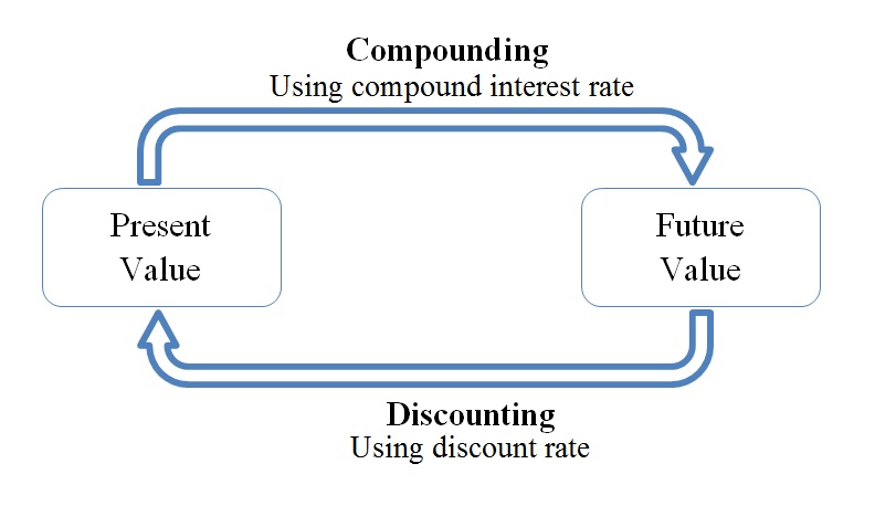
Discounting and Compounding
Compounding
In order to compare different alternatives in an economic evaluation, they should have the same base (equivalent base). Compound interest is a method that can help applying the time value of money. For example, assume you have 100 dollars now and you put it in a bank for interest rate of 3% per year. After one year, the bank will pay you . Then, you will put the 103 dollars in the bank again for another year. One year later, you will have . If you repeat this action over and over, you will have:
Which can be written as:
In general:
The value of money after nth period of time can be calculated as:
Which F is the future value of money, P is the money that you have at the present time, and i is the compound interest rate.
Example 1-1:
Assume you put 20,000 dollars (principal) in a bank for the interest rate of 4%. How much money will the bank give you after 10 years?
So the bank will pay you 29604.8 after 10 years.
Discounting
In economic evaluations, “discounted” is equivalent to “present value” or “present worth” of money. As you know, the value of money is dependent on time; you prefer to have 100 dollars now rather than five years from now, because with 100 dollars you can buy more things now than five years from now, and the value of 100 dollars in the future is equivalent to a lower present value. That's why when you take loan from the bank, the summation of all your installments will be higher than the loan that you take. In an investment project, flow of money can occur in different time intervals. In order to evaluate the project, time value of money should be taken into consideration, and values should have the same base. Otherwise, different alternatives can’t be compared.
Assume you temporarily worked in a project, and in the end (which is present time), you are offered to be paid 2000 dollars now or 2600 dollars 3 years from now. Which payment method will you chose?
In order to decide, you need to know how much is the value of 2600 dollars now, to be able to compare that with 2000 dollars. To calculate the present value of a money occurred in the future, you need to discount that to the present time and to do so, you need discount rate. Discount rate, i, is the rate that money is discounted over the time, the rate that time adds/drops value to the money per time period. It is the interest rate that brings future values into the present when considering the time value of money. Discount rate represents the rate of return on similar investments with the same level of risk.
So, if the discount rate is i=10% per year, it means the value of money that you have now is 10% higher next year. So, if you have P dollars money now, next year you will have and if you have F dollars money next year, your money is equivalent to dollars at present time.
Going back to the example, considering the discount rate of 10%:
We can calculate the present value of $2600 occurred 3 years from now by discounting it year by year back to the present time:
Value of 2600 dollars in the 2nd years from now
Value of 2600 dollars in the 1st years from now
Value of 2600 dollars at the present time
So, it seems at the discount rate of i=10%, present value of 2600 dollars in 3 years equals 1953.42 dollars, and you are better off, if you accept the 2000 dollars now.
With the following fundamental equation, present value of a single sum of money in any time in the future can be calculated. It means a single sum of money in the future can be converted to an equivalent present single sum of money, knowing the interest rate and the time. This is called discounting.
P: Present single sum of money.
F: A future single sum of money at some designated future date.
n: The number of periods in the project evaluation life (can be year, quarter or month).
i: The discount rate (interest rate).
Example 1-2:
Assuming the discount rate of 10 %, present value of 100 dollars which will be received in 5 years from now can be calculated as:
You can see how time and discount rate can affect the value of money in the future. 62.1 dollars is the equivalent present sum that has the same value of 100 dollars in five years under the discount rate of 10%
Note:
The concept of compounding and discounting are similar. Discounting brings a future sum of money to the present time using discount rate and compounding brings a present sum of money to future time.
Compound Interest Formulas I
Example 1-2 was about one single sum; what if you want to add some savings to your bank account each year? So, we need to learn some more techniques to be prepared for real-world economic evaluations. First, take a look at Figure 1-2. It can help us to better understand the investment evaluation problems.
| P | A | A | A | A | A | F | ||
|
|
||||||||
| 0 | 1 | 2 | 3 | ... | n-1 | n | ||
Figure 1-2: Time diagram
The horizontal line represents the time. The left-hand end shows the present time and the right-hand end shows the future. The numbers below the line (1, 2, 3, …, n) are time periods. Above each time period, there is a sum A, which shows the money that occurs in that time period; here, we assume all of them are equal payments, so:
A is a uniform series of equal payments at each compounding period;
P is a present single sum of money at the time zero;
F is a future sum of money at the end of period n. And i is the compound interest rate.
In order to understand an economic evaluation problem we have to determine:
- How much money is given?
- When is the money given (where on the timeline)?
- What is the time period (year, quarter, or month)?
- What is the interest rate?
- What needs to be calculated?
Following these steps, we just need to use the proper equation to solve the problem. Based on the unknown (asked) variable, there are six basic categories of problems here:
- F (future value) needs to be calculated from given P
- F (future value) needs to be calculated from given A
- P (present value) needs to be calculated from given F
- P (present value) needs to be calculated from given A
- A (uniform and equal period values) needs to be calculated from given F
- A (uniform and equal period values) needs to be calculated from given P
Table 1-1 displays a method of notation that can help summarize the given information and avoid confusion.
| To be Calculated Quantity | Given Quantity | Appropriate Factor (symbol) | Relationship | |
|---|---|---|---|---|
| 1 | F | P | ||
| 2 | P | F | ||
| 3 | F | A | ||
| 4 | A | F | ||
| 5 | P | A | ||
| 6 | A | P |
Note: “/” in the Appropriate Factor (symbol) column is not a division operator, the entire or , … is a factor (symbol). The first letter shows the variable that needs to be calculated and the second letter shows the given variable. The two subscripts on each factor are the given period interest rate, i, followed by the number of interest compounding periods, n.
The new notation helps us summarize the problem. The factor actually give a gives us a coefficient that when multiplied by given parameter, gives the unknown parameter.
All time value of money calculations involves writing an equation or equations to calculate F, P, or A. Each of terms in the column “Appropriate Factor (symbol)” has a name that you will learn later in this course.
Please watch the following (4:32) video:
PRESENTER: Hello. In this video, I'm going to summarize the basic economic evaluation problems, and I will explain how to approach each one. When facing a problem, we have to ask these five main questions. How much money is given? When is the money given, or where on the timeline? What is the time period, year, quarter, or month? What is the interest rate? What needs to be calculated?
The next step in approaching the problem is to draw the timeline. Here, as you can see, the horizontal line represents the time. The left hand end shows the present time and right hand end shows the future. Numbers below the line 0, 1, 2, 3, and n are time periods.
Now, let's add the variables. P on the left hand side is the present single sum of money at time zero. This is the amount of money that is received or paid at the present time, at time zero, at year zero or month zero. We could also write it-- write this P above the time zero. It would be the same.
The other variable is F, which is the future sum of money at the end of the period n. This is the amount of money that is received or paid in the future in the end of the end period, end year, end month. We could also write it above the end year, it's the same. The other parameter is A.
Above each time period starting from year one to year n, there is an A, which are called uniform series of equal payments at each compounding period. These A's show the money that has occurred, that is paid or received in those time periods. Here we assume all of them are equal payments.
When we face a problem, we just need to use the proper equation to solve it. And the next step is to figure out what type of problem we have. Based on given and unknown variables, there are six main categories of problems. In first category, P, money paid or received at the present time is given, and F, future value of that amount needs to be calculated.
Second category, F is given and P needs to be calculated. In third category, F needs to be calculated from given A, uniform and equal series of payments. In fourth category, A needs to be calculated from given f. Fifth category, P, present value, needs to be calculated from given A, and in sixth category, a needs to be calculated from given P. Note that in each type, we have only two money variables.
You can see these six categories in this table. The first column shows the unknown variable, the variable that needs to be calculated. The second column shows the given variable. And the third column shows the appropriate factor. Factor is just a notation, a symbol to summarize the problem.
The slash sign is not a division operator. The first letter on the left hand side of the slash sign shows the variable that needs to be calculated. And the second letter on the right hand side of the slash sign shows the given variable. The two subscripts on each factor are period interest rate, i, followed by the number of interest compounding period, n.
1. Single Payment Compound-Amount Factor
The first category of six categories that were introduced explains the situation that the present value of money is given and asks you to calculate the future value according to the given interest rate of i per period and n period from now. This problem can be summarized with the factor (symbol) of and can be shown as:
| P | _ | _ | _ | _ | _ | F=? | ||
|
|
||||||||
| 0 | 1 | 2 | 3 | ... | n-1 | n | ||
Figure 1-3: Single Payment Compound-Amount Factor, F/Pi,n
As explained earlier, the future value of money after n period with an interest rate of i can be calculated using the Equation 1-1: which can also be written regarding Table 1-1 notation as: . The mathematical expression is called the “single payment compound-amount factor."
Compound Interest Formulas II
3. Uniform Series Compound-Amount Factor
The third category of problems in Table 1-5 demonstrates the situation that equal amounts of money, A, are invested at each time period for n number of time periods at interest rate of i (given information are A, n, and i) and the future worth (value) of those amounts needs to be calculated. This set of problems can be noted as . The following graph shows the amount occurred. Think of it as this example: you are able to deposit A dollars every year (at the end of the year, starting from year 1) in an imaginary bank account that gives you i percent interest and you can repeat this for n years (depositing A dollars at the end of the year). You want to know how much you will have at the end of year nth.
| 0 | A | A | A | A | F=? | ||
|
|
|||||||
| 0 | 1 | 2 | ... | n-1 | n | ||
Figure 1-4: Uniform Series Compound-Amount Factor,
In this case, utilizing Equation 1-2 can help us calculate the future value of each single investment and then the cumulative future worth of these equal investments.
Future value of first investment occurred at time period 1 equals
Note that first investment occurred in time period 1 (one period after present time) so it is n-1 periods before the nth period and then the power is n-1.
And similarly:
Future value of second investment occurred at time period 2:
Future value of third investment occurred at time period 3:
Future value of last investment occurred at time period n:
Note that the last payment occurs at the same time as F.
So, the summation of all future values is
By multiplying both sides by (1+i), we will have
By subtracting first equation from second one, we will have
which becomes:
then
Therefore, Equation 1-3 can determine the future value of uniform series of equal investments as . Which can also be written regarding Table 1-5 notation as: . Then .
The factor is called “Uniform Series Compound-Amount Factor” and is designated by F/Ai,n. This factor is used to calculate a future single sum, “F”, that is equivalent to a uniform series of equal end of period payments, “A”.
Note that n is the number of time periods that equal series of payments occur.
Please review the following video, Uniform Series Compound-Amount Factor (3:42).
PRESENTER: In the third category, equal amounts of money A are enlisted pay to receive at each time period for n number of time periods. n can be years or months, and interest rate is i. And the question asks you to calculate the future value of these payments, a single sum of money that is equivalent to all these series of payments A. Here, given information are A, n, and i. And F is the unknown parameter. These sets of problems can be displayed with the factor F slash A, or F/A. Again, the left side of this slash sign is the unknown parameter F, and the right side is the given variable, which is A.
Here, you can see the equation to calculate F from A, i and n. The mathematical proof of this equation is straightforward, and they explain it in Lesson One. We can write this equation, regarding the factor notation, F equals A multiply the factor. This factor is called uniform series compound-amount factor. And it is used to calculate the future single sum F that is equivalent to uniform series of equal ends of period payments A.
Let's work on an example to see how this factor can be used. Assume you save $4,000 per year and deposit it, in the end of the year, in an imaginary saving account or some other investment that gives you 6% interest rate per year, compounded annually, for 20 years, starting from year 1 to year 20th. And you want to know how much money will you have in the end of the 20th year.
First, we draw the time line. Left-hand side is the present time. We don't have anything there. Note that your investment, it starts from year 1 to year 20th. If there is no extra information in the question, and question says you invest for 20 years, you need to assume your investment, it starts from year 1. So there is no payment at present time, or year zero.
Right-hand side is the future time, which is a single amount future value, and it is unknown. Your investment takes 20 years, so n equals 20. And above each year, you have to write $4,000, because you have a payment of $4,000 in the end of each year. So A equals $4,000, n number of years is 20, i interest rate 6%, and F needs to be calculated.
And F equals A times the factor F/A. In this factor, i is 6% and 20. And we use the equation to calculate the F. And we find the answer. So if you invest $4,000 per year for 20 years, with 6% interest rate, you will have about $147,000 at the end of the 20th year.
Example 1-3:
Assume you save 4000 dollars per year and deposit it at the end of the year in an imaginary saving account (or some other investment) that gives you 6% interest rate (per year compounded annually), for 20 years. How much money will you have at the end of the 20th year?
| 0 | $4000 | $4000 | $4000 | $4000 | F=? | ||
|
|
|||||||
| 0 | 1 | 2 | ... | 19 | 20 | ||
So
A =$4000
n =20
i =6%
F=?
Please note that n is the number of equal payments.
Using Equation 1-3, we will have
So, you will have 147,142.4 dollars at 20th year.
| Factor | Name | Formula | Requested variable | Given variables |
|---|---|---|---|---|
| F/Ai,n | Uniform Series Compound-Amount Factor | F: Future value of uniform series of equal investments | A: uniform series of equal investments n: number of time periods i: interest rate |
4. Sinking-Fund Deposit Factor
The fourth group in Table 1-5 is similar to the third group but instead of A as given and F as unknown parameters, F is given and A needs to be calculated. This group illustrates the set of problems that ask you to calculate uniform series of equal payments (or investment), A, to be invested for n number of time periods at interest rate of i and accumulated future value of all payments equal to F. Such problems can be noted as and are displayed in the following graph. Think of it as this example: you are planning to have F dollars in n years and there is a saving account that can give you i percent interest. You want to know how much you have to deposit every year (at the end of the year, starting from year 1) to be able to have F dollars after n years.
| 0 | A=? | A=? | A=? | A=? | F | ||
|
|
|||||||
| 0 | 1 | 2 | ... | n-1 | n | ||
Figure 1-5: Sinking-Fund Deposit Factor,
Equation 1-3 can be rewritten for A (as unknown) to solve these problems:
Equation 1-4 can determine uniform series of equal investments, A, given the cumulated future value, F, the number of the investment period, n, and interest rate i. Table 1-5 notes these problems as: . Then . The factor is called the “sinking-fund deposit factor”, and is designated by . The factor is used to calculate a uniform series of equal end-of-period payments, A, that are equivalent to a future sum F.
Note that n is the number of time periods that equal series of payments occur.
Please watch the following video, Sinking Fund Deposit Factor (4:42).
PRESENTER: The fourth group is similar to the third one. But A is the unknown and F is the given variable. This set of problems asks you to calculate uniform series of equal payments, A, to be invested for n number of time periods at interest rate of i. And the accumulated future value of all payments or equivalent future value is F.
This set of problems can be summarized with the factor A over F or A slash F. The left side of this last sign is the unknown parameter. Here it is A. And the right side is the given variable, which is F.
Equation 1-3 for uniform series compound amount factor can be rewritten for A as unknown to solve these problems, which gives the Equation 1-4. Equation 1-4 can determine uniform series of equal investments, A, for accumulated future value, F, number of investment period n and interest rate i.
We can write this equation according to the factor notation, A equals F times the factor A over F. This factor is called the Sinking-Fund Deposit Factor. And it is displayed by A slash F. The factor is used to calculate the uniform series of equal end of the period payments, A, that are equivalent to a future sum, F.
For example, referring to example 1-7 in previous video, let's say you plan to have $200,000 after 20 years. And you are offered an investment, which can be the imaginary savings account, that gives you 6% per year compound interest rates. And you want to know how much money, equal payments, you need to save each year, or invest-- deposit in your account in the end of each year.
So in summary, you want to have $200,000 after 20 years. And you can invest your money with 6% interest rate. The question is, how much you need to invest per year?
Again, the first step is drawing the time line. Left-hand side is the present time. We won't have any payment. So there is no payment at present time or time zero. Right-hand side is the future. And you want to have a single amount of $200,000. So you write $200,000 in the 20th year, or in the end of right-hand side of the time line.
Note that $200,000 has the same time dimension as the last payment, A. Both are in the year 20th. Your investment takes 20 years, so n equals 20. And above each year, you have to write A, which is unknown and needs to be calculated.
So F equals $200,000. n number of years is 20. i, interest rate, 6%. And A needs to be calculated.
We can use the factor notation to summarize the equation. In this factor, i is 6%, n is 20, and F is given, and A needs to be calculated. And we calculate the result. So if you want to have $200,000 in 20 years from now with 6% interest rate, you will need to invest equal amounts of $5,437 per year at the end of each year for 20 years, starting from year one.
Example 1-4:
Referring to Example 1-3, assume you plan to have 200,000 dollars after 20 years, and you are offered an investment (imaginary saving account) that gives you 6% per year compound interest rate. How much money (equal payments) do you need to save each year and invest (deposit it to your account) in the end of each year?
| 0 | A=? | A=? | A=? | A=? | F=200,000 | ||
|
|
|||||||
| 0 | 1 | 2 | ... | 19 | 20 | ||
So
F=$200,000
n=20
i=6%
A=?
Using Equation 1-4, we will have
So, in order to have 200,000 dollars at 20th year, you have to invest 5,436.9 dollars in the end of each year for 20 years at annual compound interest rate of 6%.
| Factor | Name | Formula | Requested variable | Given variables |
|---|---|---|---|---|
| Sinking-Fund Deposit Factor | A: Uniform series of equal end-of-period payments | F: cumulated future value of investments n: number of time periods i: interest rate |
Note that
Compound Interest Formulas III
5. Uniform Series Present-Worth Factor
The fifth group in Table 1-5 covers a set of problems that uniform series of equal investments, A, occurred at the end of each time period for n number of periods at the compound interest rate of i. In this case, the cumulated present value of all investments, P, needs to be calculated. In summary, P is unknown and A, i, and n are given parameters. And the problem can be noted as and displayed as:
| P=? | A | A | A | A | 0 | ||
|
|
|||||||
| 0 | 1 | 2 | ... | n-1 | n | ||
Figure 1-6: Uniform Series Present-Worth Factor,
If we replace substitute F in Equation 1-3 from Equation 1-2, we will have the present value as:
then,
Equation 1-5 gives the cumulated present value, P, of all uniform series of equal investments, A, as . And also can be noted as: .The factor is called the “uniform series present-worth factor” and is designated by . This factor is used to calculate the present sum, P that is equivalent to a uniform of equal end of period payments, A. Then
Note that n is the number of time periods that equal series of payments occur.
Please review the following video, Uniform Series Present Worth Factor (Time 3:35).
PRESENTER: The fifth group covers the set of problems that P is a known parameter, A, i and n are given variables. In these problems, we have uniform series of equal investments, A, in the end of each time period, for n number of periods, at the compound interest rate of I.
And the problem asks you to calculate the accumulated present value of all investments, P. We can summarize these questions using the factor notation. P is the unknown variable, and should be on the left side. And A is the given, and should be written on the right side.
As explained before, Equation 1-3 returns the future value, F, from A, i and n. And Equation 1-2 calculates the future value, F, from present value, P, interest rates, i and n number of periods. So if we substitute F in Equation 1-3 from Equation 1-2, we will have this new equation-- 1-5. This equation gives us the accumulated present value of equal series payments, A, paid for n period, at interest rate of i.
Equation 1-5 can also be written according to factor notation. P equals A times the factor P over A. This factor is called Uniform Series Present-Worth Factor, which is used to calculate the presence on P that is equivalent to a uniform series of equal payments, end of the period payments, A.
For example, what would be the present value of 10 uniform investments of $2,000, invested at the end of each year, for interest rate of 12%, compounded annually? First, we draw the time line. Left hand side is a present time, time zero payment, which needs to be calculated. N equals 10, because there are 10 uniform investments.
So we have 10 years. And above each year, we have $2,000, starting from year one to year 10. So A equals $2,000, n is 10, and interest rate is 12%. Using the factorization, P equals A, multiply the factor-- i is 12%, and n is 10. And the result.
So if you save $2,000 per year, at the end of each year for 10 years, starting from year one to year 10, the accumulated money is equal to $11,300 at present time. It has the same value as $11,300 at the present time.
Example 1-5:
Calculate the present value of 10 uniform investments of 2000 dollars to be invested at the end of each year for interest rate 12% per year compound annually.
| P=? | A=$2000 | A=$2000 | A=$2000 | A=$2000 | 0 | ||
|
|
|||||||
| 0 | 1 | 2 | ... | 9 | 10 | ||
So,
A =$2000
n =10
i =12%
P=?
Using Equation 1-5, we will have:
Note that we use the factor when we have equal series of payments. i is the interest rate and n is the number of equal payments. There is an important assumption here, the first payment has to start from year 1. In that case will return the equivalent present value of the equal payments.
Now let's consider the case that we have equal series of payments and the first payment doesn't start from year 1. In that case the factor will give us the equivalent single value of equal series of payments in the year before the first payment. However, we want the present value of them (at year 0). So, we need to multiply that with the factor and discount it to the present time (year 0).
Example:
| P=? | A=$2000 | A=$2000 | A=$2000 | 0 | |||
|
|
|||||||
| 0 | 1 | 2 | ... | 10 | 11 | ||
Note that there are 10 equal series of $2,000 payments. But the first payment is not in year 1. The factor returns the equivalent value of these 10 payments to the year before the first payment, which is year 1.
| P=? | $2000(P/A12%,10) | 0 | |||||
|
|
|||||||
| 0 | 1 | 2 | ... | 10 | 11 | ||
However, we want the present value. So, we need to discount the value by one year to have the present value of 10 equal payments.
| P=? | $2000(P/A12%,10)(P/F12%,1) | 0 | |||||
|
|
|||||||
| 0 | 1 | 2 | ... | 10 | 11 | ||
Example: Now consider the the following case that the first payment starts at year 3:
| P=? | A=$2000 | A=$2000 | A=$2000 | 0 | ||||
|
|
||||||||
| 0 | 1 | 2 | 3 | ... | 10 | 12 | ||
| Factor | Name | Formula | Requested variable | Given variables |
|---|---|---|---|---|
| Uniform Series Present-Worth Factor | P: Present value of uniform series of equal investments | A: uniform series of equal investments n: number of time periods i: interest rate |
6.Capital-Recovery Factor
The sixth group in Table 1-5 belongs to set of problems that A is unknown and P, i, and n are given parameters. In this category, uniform series of an equal sum, A, is invested at the end of each time period for n periods at the compound interest rate of i. In this case, the cumulated present value of all investments, P, is given and A needs to be calculated. It can be noted as .
| P | A=? | A=? | A=? | A=? | 0 | ||
|
|
|||||||
| 0 | 1 | 2 | ... | n-1 | n | ||
Figure 1-7: Capital-Recovery Factor,
Equation 1-5 can be rewritten for A (as unknown) to solve these problems:
Equation 1-6 determines the uniform series of equal investments, A, from cumulated present value, P, as . The factor is called the “capital-recovery factor” and is designated by A/Pi,n. This factor is used to calculate a uniform series of end of period payment, A that are equivalent to present single sum of money P.
Note that n is the number of time periods that equal series of payments occur.
Please watch the following video, Capital Recovery Factor (Time 3:37).
PRESENTER: The sixth group belongs to the set of problems that A is unknown and P, i, and n are given parameters. This category is similar to the fifth group, but P is given and A needs to be calculated. In this category of problems, we know the present value P, or accumulated present value of all payments. And we want to calculate the uniform series of equal sum A that are invested in the end of each time period for n periods at the compound interest rate of i.
So we have present value P, and we want to calculate equivalent A, given interest rate of i and number of periods n. The proper factor to summarize these questions is A over P, or A/P. A is the unknown variable, is on the left side, and P, given variable, on the right side.
Equation to calculate A is straightforward. We just need to rewrite the equation in 1-5 for A as unknown, and we will have equation 1-6 that calculates A from P, i, and n. If we write the equation 1-6 according to the factor notation, we will have factor A over P. The factor is called capital recovery factor and is used to calculate uniform sales of end of period payments A that are equivalent to present single sum of money P.
Let's work on this example. We want to know the uniform series of equal investment for five years at interest rate of 4% which are equivalent to $25,000 today. Let's say you want to buy a car today for $25,000, and you can finance the car for five years and 4% of interest rate per year, compounded annually. And you want to know how much you have to pay each year.
First, we draw the timeline. Left side is the present time, which we have $25,000. n equals 5, and above each year, starting from year one to year five, we have A that has to be calculated. For the factor, we have i equal 4% and n is five and the result, which tells us $25,000 at present time is equivalent to five uniform payments of $5,616 starting from year one to year five with 4% annual interest rate. Or $25,000 at present time has the same value of five uniform payments of $5,616 starting from year one to year five with 4% annual interest rate.
Example 1-6:
Calculate uniform series of equal investment for 5 years from present at an interest rate of 4% per year compound annually which are equivalent to 25,000 dollars today. (Assume you want to buy a car today for 25000 dollars and you can finance the car for 5 years with 4% of interest rate per year compound annually, how much you have to pay each year?)
| P=$25,000 | A=? | A=? | A=? | A=? | A=? | 0 | |
|
|
|||||||
| 0 | 1 | 2 | 3 | 4 | 5 | ||
Using Equation 1-6, we will have:
So, having $25,000 at the present time is equivalent to investing $5,615.68 each year (at the end of the year) for 5 years at annual compound interest rate of 4%.
| Factor | Name | Formula | Requested variable | Given variables |
|---|---|---|---|---|
| Capital-Recovery Factor | A: uniform series of equal investments | P: Present value of uniform series of equal investments n: number of time periods i: interest rate |
Note that
Using these six techniques, we can solve more complicated questions.
Example 1-7:
Assume a person invests 1000 dollars in the first year, 1500 dollars in the second year, 1800 dollars in the third year, 1200 dollars in the fourth year and 2000 dollars in the fifth year. At an interest rate of 8%:
1) Calculate time zero lump sum settlement “P”.
2) Calculate end of year five lump sum settlement “F”, that is equivalent to receiving the end of the period payments.
3) Calculate five uniform series of equal payments "A", starting at year one, that is equivalent to above values.
| P=? | 1000 | 1500 | 1800 | 1200 | 2000 | F=? | |
|
|
|||||||
| 0 | 1 | 2 | 3 | 4 | 5 | ||
1) Time zero lump sum settlement “P” equals the summation of present values:
2) End of year five lump sum settlement “F”, that is equivalent to receiving the end of the period payments equals the summation of future values:
Please note that in the factor subscript, n is the number of time period difference between F (the time that future value has to be calculated) and P(the time that the payment occurred). For example, 1800 payment occurs in year 3 but we need its future value in year 5 (2 year after) and time difference is 2 years. So, the proper factor would be: .
3) Uniform series of equal payments "A" can be calculated from either P or F :
or
Example 1-8: repeat your calculations for the following payments:
| P=? | 800 | 1000 | 1000 | 1600 | 1400 | F=? | |
|
|
|||||||
| 0 | 1 | 2 | 3 | 4 | 5 | ||
1) Time zero lump sum settlement “P” equals the summation of present values:
2) End of year five lump sum settlement “F”, that is equivalent to receiving the end of the period payments equals the summation of future values:
3) Uniform series of equal payments "A" can be calculated from either P or F:
or
Cash Flow
The first step in conducting an economic evaluation analysis is to understand the concept of “cash flow.” “Cash flow” represents the net inflow or outflow of money during a given period of time that can be month, quarter, or year. Cash flow can be reported as before-tax cash flow (BTCF) and after-tax cash flow (ATCF).
Operating Profit or EBITDA = Gross Revenue or Savings – Operating Expenses
Before tax Cash Flow = Operating Profit or EBITDA – Capital Expenditure
After tax Cash Flow = Before tax Cash Flow – Income Tax Expenditure
Which is formatted as:
Gross Revenue or Savings
– Operating Expenses
_____________________________
Operating Profit or EBITDA
– Capital Expenditure
_____________________________
Before tax Cash Flow
– Income Tax Expenditure
_____________________________
After tax Cash Flow
EBITDA : Earnings before interest, taxes, depreciation, and amortization
Example 1-9:
Assume an investment project for which you need to invest 20 and 15 million dollars in year 0 and year 1 (you can think of it as 20 million dollars now and 15 million dollars next year) to build a facility. In year 2, the plant will start producing and you can make revenue by selling the products. Each year, starting from year 2, operating costs and tax have to be paid. Project net cash flow can be calculated as:
| Year 0 | Year 1 | Year 2 | Year 3 | Year 4 | Year 5 | Year 6 | Year 7 | Year 8 | |
|---|---|---|---|---|---|---|---|---|---|
| Revenue | 18 | 20 | 22 | 24 | 26 | 28 | 30 | ||
| Operating Cost | -4 | -4 | -4 | -5 | -6 | -8 | -10 | ||
| Capital Cost | -20 | -15 | |||||||
| Tax Cost | -3 | -4 | -5 | -6 | -7 | -8 | -9 | ||
| Project Cash Flow | -20 | -15 | 11 | 12 | 13 | 13 | 13 | 12 | 11 |
Each column stands for a time period (that can be year, quarter, month, …) and each cell shows the inflow or outflow of money. Investment cash flow in any year represents the net difference between inflows of money from all sources, minus investment outflows of money from all sources. The cash flow for this project for all years is calculated in the last row.
As you can see, all the costs (Capital Cost, Operating Cost, Tax, ...) are entered with the negative sign in the table, and then summation of each column gives the net cash flow in that year. The negative cash flow incurred in years 0 and 1 will be paid off by positive cash flows in years 2 through 8.
Discounted Cash Flow (DCF)
If future cash flow is discounted, we can have cash flow in terms of present value, which is called discounted cash flow (DCF). As explained before, DCF considers the time value of money and applies it to the inflow and outflow of money occurred in the future. DCF is a tool that enables us to compare the future cash flow with the present value of money.
Different investment projects have different cash flows that happen in different time intervals in the future and DCF can give an assessment to decide which project is more profitable. DCF brings the future amounts to a same base that is easily understandable for decision makers. For example, assume you have two options: investing your money in Project A that gives you 1000 dollars every year from 2025 to 2035 or investing in Project B that gives you 1500 dollars every year from 2030 to 2040. Which project will you choose? DCF is a tool that can help you finding the answer. DCF can also be used to estimate the value of a company based on its future performance.
Example 1-10:
Please calculate the discounted cash flow from Example 1-9 assuming:
1) Discount rate = 10%
2) Discount rate = 12%
3) Discount rate = 15%
Assuming discount rate = 10%:
We can repeat the same procedure for discount rate = 12% and 15%. Table 1-2 shows the results.
| Year | 0 | 1 | 2 | 3 | 4 | 5 | 6 | 7 | 8 |
|---|---|---|---|---|---|---|---|---|---|
| Project Cash Flow | -20 | -15 | 11 | 12 | 13 | 13 | 13 | 12 | 11 |
| DCF (discount rate = 10%) | -20 | -13.6 | 9.1 | 9.0 | 8.9 | 8.1 | 7.3 | 6.2 | 5.1 |
| DCF (discount rate = 12%) | -20 | -13.4 | 8.8 | 8.5 | 8.3 | 7.4 | 6.6 | 5.4 | 4.4 |
| DCF (discount rate = 15%) | -20 | -13 | 8.3 | 7.9 | 7.4 | 6.5 | 5.6 | 4.5 | 3.6 |
Net Present Value (NPV)
Now, all the DCFs in Table 1-3 have the same base, which is present value, consequently it’s possible to add them together and create a new criterion for project evaluation. The criterion which represents this summation is called net present value (NPV). NPV is the cumulative present worth of positive and negative investment cash flow using a specified rate to handle the time value of money.
Example 1-11:
Please calculate the NPV for the cash flow in Example 1-9 assuming:
1) Discount rate = 10%
2) Discount rate = 12%
3) Discount rate = 15%
Discount rate = 10%:
Assuming discount rate = 12%:
Assuming discount rate = 15%:
As you can see, the discount rate has a substantial effect on the project NPV, higher discount rates give lower NPV of the cash flow. The other important factor is the time. The closer the money is to present time, the higher present value it has, which affects the NPV.
Example 1-12:
Assume you have two alternative projects to invest your 600 dollars. The cash flow in Project A and Project B are shown in Table 1-4. Which project do you choose if the discount rate is 10%?
| Year | 0 | 1 | 2 | 3 |
|---|---|---|---|---|
| Project A Cash Flow | -600 | 500 | 300 | 200 |
| Project B Cash Flow | -600 | 200 | 300 | 500 |
Please note that two projects have similar numbers for cash flow but they happen in different times. DCFs are displayed in following table.
| Year | 0 | 1 | 2 | 3 |
|---|---|---|---|---|
| DCF for Project A | -600 | 454.5 | 247.9 | 150.3 |
| DCF for Project B | -600 | 181.8 | 247.9 | 375.7 |
This example shows how time affects the NPV of an investment project. As displayed in Table 1-5 and NPV calculations, Project A which has higher positive cash flows in closer time has higher NPV and it is a better alternative for investment than Project B.
Minimum Rate of Return
The terms “minimum rate of return," “hurdle rate," “discount rate," “minimum discount rate," and “opportunity cost of capital” are interchangeable with the term “cost of capital” as used in this course and in common practice. These terms should not be confused with the “financial cost of capital,” which is the cost of raising money by borrowing or issuing a bond, debenture, common stock or related debt/equity offerings. When the usual situation of capital rationing exists, the “opportunity cost of capital” generally is larger than the “financial cost of capital."
Microsoft Excel Tutorial
Microsoft Excel is a useful, convenient and widely used software for financial calculations and analysis that you will learn in this course. So, you are expected to learn and use required skills to utilize such tools.
If you do not have access to a commercial-grade spreadsheet program (such as Excel or OpenOffice), you can find free Spreadsheet applications available through Google Drive or a similar online tool. Following links include tutorials for Google Spreadsheet.
• Google Spreadsheet Tutorial from Google [1]
• Google Spreadsheet Tutorial from YouTube [2]
And also if you search online for “Google Spreadsheet Tutorial”, you can find some other good tutorial websites and videos.
Microsoft Excel
If it is the first time you are using Excel, please refer to the following video for a tutorial of Microsoft EXCEL 2010. (Time 10:00)
Please note that you need to open this video in YouTube [3]. (transcript [4])
You can follow the tutorial step by step to be a master of Excel 2010, which is a very powerful tool in the industry, business, and academia.
Tutorial for calculating present Value using Microsoft Excel (Time 7:35):
PRESENTER: Hi, guys. Welcome to subjectmoney.com. This is our video series of Excel tips and tricks. And in this video, we're going to go over how to find the present value of multiple future cash flows of different amounts.
Now, I'm already assuming that you pretty much know, have a decent understanding, of present value. But just in case, I'll kind of explain it. Basically, what present value is is most people know that a certain amount of money in the future, say $100 in the future, is not equivalent, does not have the same value as $100 today.
And the reason why is because if you had $100 today, you could invest that money. And it would earn interest. It would give you a return, making it worth more than $100 in the future. So why would a $100 in the future be worth $100 today?
Kind of a simple explanation of it is just to imagine that you had an account that you earned 10% interest on. OK. If you put $100 on in account, one year from today, it would be worth $110. And two years from today, it would be worth $121.
So, basically, what we're saying, if 10% is your discount rate, that's your opportunity cost. $121 two years from today, discounted the present value today, would be worth $100 if your opportunity to invest was 10%. And $110 one year from today, if you had a 10% account that you could invest in, would only be worth $100.
So that's kind of the concept of present value. All right, so what we're going to do, let's just go ahead and move into the purpose of this video. I'm gonna go over how to find the present value using Microsoft Excel.
OK. So you can see here I have a little chart. This right here stands for today, today plus one, which means one year from today, two years from today, three years from today, four years from today, and so on. And for each year, I have an expected cash inflow.
So like one year from today, I'm expecting to receive $100. Seven years from today over here, I'm expecting to receive $1,000. So we want to find the present value of all these cash flows. Because this could be one single investment maybe that's bringing in these cash flows. So what is the present value of this investment?
All right, so first I'll go to the long way to do it. I could go here and just enter in the formula for each cash flow. So that would be equals the cash flow I'm referring to that cell, F8, the cash flow, divided by-- so the form is going to be the cash flow divided by 1 plus the rate of return. That's our opportunity cost or our discount rate.
Now, I'm going to hit F4. Because we don't want this cell. When we drag this formula over, we want this to stay put. And we want to stay locked into that cell. But this, we're not doing it. Because when we drag these over, we need to be referring to each cell.
All right, so we close parentheses, and then I put the power of 1. And that gives a present value of $92.59. I need a new mouse. All right, let me do the Show Formula real quick.
OK. So I'm going to go ahead, and I can drag this over. And this is basically a lump sum present value formula in each one of these. Because we're finding the present value of a single cash flow.
So I can drag this over. Now, what I have to do, though, is this cash flow is two years from today. So it needs to be discounted back two years. So it's going to be the cash flow divided by 1 plus the discount rate to the power of 2, or however many years it is until we receive it.
So over here, it's going to be discounted three years. And we will do that all the way until our final cash flow. And we need to go in here and change this formula four years, five years, six years, and seven years.
All right. Now, so you can see we have the formula for each cash flow. Now, I'm going to get out of the Show Formula mode. And now you can see in this row, we have our present value of each cash flow.
OK. So the present value of multiple future cash flows is going to be the sum of the present values of each cash flow. So =sum, that's the sum formula. And then all we have to do is we're doing the sum of-- and in parentheses, we highlight all of these numbers, the sum of all the present values.
So our present value is $2,260.80. All right, now that was the long way. I'm going to go ahead, and I'm going to show you the short version in Excel. And that's using the Net Present Value mode.
Now, I'm going to go ahead and delete this row, because we don't even need it. So right here, we have all of our cash flows. All we're going to do is we hit =npv, which stands for Net Present Value.
And then right here, you can see it tells us what to do. So it says to enter the rate. So we refer back to our rate. And it says enter a comma. So we hit a comma. And now, we're going to add up all of our cash flows.
Oh, no, no, no. Sorry. We're not going to add them up. Comma-- click them and a comma, and then close the parentheses. And you can see the net present value is $2,260.80, the same as what we had before, except for we didn't have to do all of those calculations.
So again, I'll show you the formula. And you can see it. It =npv, the rate, and then each cash flow to be received. And you cannot skip years.
Even if one of these years doesn't have a-- maybe you don't expect any money. You still have to enter it in. Because say right here I made this 0, it's going to change our net present value. But we still need to have that cell entered into this formula.
Because it's discounting each one of these back. It's discounting this one one year. If we were to skip it, then it wouldn't discount it back the right amount of years.
All right, so that concludes this tutorial of how to find the present value of multiple future cash flows. Make sure to visit our website at subjectmoney.com and to share our videos. And stay tuned, because we have plenty more coming in the future. Thanks, bye.
And also, these two following links (Times: 5:15 and 7:50):
PRESENTER: Here I'm going to talk to you about the present value, what it is, and two really easy ways that you can get a present value in Microsoft Excel. So firstly, you may or may not know that present value essentially tells you how much to invest today, so that you have a certain amount in the future. So the basic premise of it is in 10 years, I want $50,000. OK, well, how much do I have to invest today and at what interest rate in order to get $50,000? Well, I find the interest rate by the type of investment or security that I'd like to invest, get the average interest rate, and then I can figure out exactly how much I need today in order to have that 50 grand in 10 years.
Now, we're going to talk about, like I said, two ways to do it. This is the mathematical formula right here. The present value equals the future value over 1 plus the interest rate raised to however many periods there are. I've got all the syntax listed right here with what every argument means and does. The important thing to remember is that N or number of periods can be any time frame, right, could be weeks months, days, years, quarters. The only important thing to remember is it all has to stay consistent. I'll talk about what to do when you have to separate it by months later on, but for now, let's just keep our number of periods to years. It will make everything a little bit easier for this.
So this is the basic mathematical formula. We'll talk about-- we'll actually use that in a second. The next thing is the Excel formula. So let me actually hide this real quick. The formula or the function that we're going to be using is the present value function, and it has a number of arguments, rate, number of periods, the payment, the future value, and the type. So let's go ahead and go through those right now.
Now, the rate is going to be the interest rate that you receive on your funds. So let's go with the most basic example, right. I want 50 grand. I've got a bank account. I'm only going to put my money within the bank accounts. So how much do I put in this bank account today to get 50 grand in 10 years? OK, so the rate that my bank is giving me is 3.25%, not so bad, right. The number of periods is going to be 10, because I want to do this for 10 years. Well, the number of payments-- well, this is not an annuity problem. I'm not going to be putting any money in my bank account. I want to know how much I'm going to make solely based on-- or solely based off the income from the interest payments.
The next thing is FV or future value. That is $50,000. How much do I want in the future? I want 50 grand. The last argument is going to be the type. This is similar to the future value function. No, actually, it's exactly the same for type, and that the type simply means whether or not you're going to receive money or input money at the beginning or the end of the period. Now if you leave type blank, it's assumed that any amount of money that's due is going to be at the end of the period. If you put a 1 for type, all of the money is going to be entered in the beginning of the period.
That's really just for an annuity, though, so we don't have to worry about that right now. So let's go ahead and use the Excel formula first. So equals PV, open parenthesis, let's get our rate, well our interest rate is right here, 3.25%, select that, comma, number of periods, 10 years, comma. Our payment, well, are we going to be paying anything into this? Am I going to add $100 every week or $1,000 every month? No. So our payment is 0 comma. Now for the future value, what do I want to do for that? Well, I want 50 grand. So that's all that we need. We don't have to worry about type, close the parenthesis, hit Enter, and you can see that we need $36,313.61.
Now, why is this negative? It's negative, because it's basically saying that you need to pay this much into your bank account today in order to get $50,000 in 10 years. Now the way that we fix that is simply double click the cell and put a negative sign in front of the function. It's not going to hurt anything. It simply makes it a positive number. Now let's go ahead and use the formula.
So this is the formula. Don't forget future value over 1 plus the interest rate raised to the number of periods. We'll do that right here very quick equals future value divided by 1 plus the interest rate raised to the number of periods, 10, close parentheses, hit Enter. And it is exactly the same. So those are the two different ways you can calculate the present value in Excel. And if you're in Excel, really you're only going to be using the present value function. So I will leave you with this.
PRESENTER: Here, I'm going to go through three examples of a typical present value problem or question in a finance class of college level, or something similar to that. Now in a previous tutorial, I've already told you what the present value function is, how to use it, and basically what present value means. So this one, I'm not going to spend too much time on that. So let's go ahead and dive right on in.
The first question is a very basic one. With an interest rate of 6%, what is the current value of $7 million if you will receive it in 15 years? This is sort of a typical example. What's worth more? So much in the future, or so much now? So let's figure out what it's actually worth in today's dollars, or using only interest rate.
So equals, pv, open parentheses. Now our rate, that's very easy. Just our interest rate of 6%. So 0.06. Now remember, when you're doing the interest rate here, you have to do it as a decimal. So 0.06. You can't type in a whole number like 6. It's not going to interpret that correctly.
The number of periods. Well, that's very easy. It's 15 years. So our number of periods-- 15 comma. Payment-- are we going to be paying into this at all, or is anyone going to be paying us at all over these 15 years? No. So payment is 0, because we're only talking about one lump sum in 15 years.
But we do know the future value. So what is the future value? $7 million. Now if you wanted, you could type it in as seven, 7, 7,000, or actually, 7 million. If you're doing this in the real world, you're going to break it down to a smaller number, such as 7, for 7 million.
So now we have the rate, right here. The number of periods-- 15. Payment is 0, because we're not going to be paying into it. It's not an annuity. And the future value is 7 million. Let's close parentheses, and hit Enter.
So it tells us that the present value is just about $3 million. Now why is this red? Why is this negative? Well, because it's assuming that this is your cash outflow. So you're going to put this 3 million in, say, a bank or a bond that pays 6%. And to put your money into something, you have to pay it out.
But to get rid of the red, the negative, simply put a little minus sign right in front of the pv function. Once you do that, you'll notice that it's a positive number once again.
All right, so let's go ahead and go to the second present value problem, on the second tab. What is the present value of putting $500 into an interest bearing account with a 2.75% interest rate for 6 years?
Now this would be considered the basic annuity problem, right? An annuity, a set of equal cash flows that you're investing at an equal rate over a period of time. So the equal cash flows being $500 invested, let's say, once a year for 6 years. So we're going to keep it easy by keeping it at years for now.
So equals, pv, open parentheses. Our rate, very easy-- 2.75%. Remember, put it in decimal form, 0.0275 comma. Number of periods, very easy. We're sticking with years for now, so 6 comma. Now the payment. Well, this time, we are going to be paying into the account every year. So the payment here is going to be 500, because that's how much we're paying in.
Now we don't have to worry about a future value for this problem, because we're not trying to figure out how much one lump sum in the future is worth today. We have many payments into the account. So close the parentheses. We got the percentage for our rate, number of periods, 6, and the payment, which is $500 going in every period.
Simply hit Enter, and we see you will end up with, or in today's dollars, it's $2,731.18. Once again, to make that positive, double-click, put a negative sign in front of it, and hit Enter. And that's it for that problem.
So just remember that since this is an annuity, we do have to fill in the argument for the payment. This one right here-- pmt. So the payment basically is what you're going to do for an annuity, right? Future value, if you want to figure out what one lump sum is worth today.
So let's go on to the third example. It's a little bit different, maybe a little bit trickier, but same premise. So if you know that you can sell something, say, an asset, in 3 years for $170,000, right? And you know that the discount rate for the asset is 4.25% per all of your due diligence and your own research. Well, then, what are you going to pay for the asset now?
So this is a present value. It's a little bit different, but the point is, how much money you going to shell out now so that you can sell it for 170 grand in the future with a 4.25% discount rate? All right, so the way to do this, exactly like before, just a different word problem.
So equals, pv, open parentheses. Once again, our rate. Well, that's easy, right? Discount rate, that's our rate-- 4.25%, so 0.0425. Now how many years would we like to discount this for? Well, we want to discount it for 3 years, so 3 for the number of periods. Number of periods-- 3.
Now for the payment, are we going to have any payments in or out? Well, let's say that this is a non-cash flow generating asset, right? Could be a mainframe for data backup, or something like that. So the payment's going to be 0.
But we do have a future value. The future value is $170,000. If you had it in thousands, you would simply write 170, but I'm going to put the full number here-- 170,000. Close the parentheses and we're done.
So all I did here, the rate is the discount rate this time. It's not called interest rate, but it's the same thing for our purposes, for what we're doing. Number of periods-- 3 years. And there is no payment. It's just a simple lump sum in 3 years, right? It's worth $170,000 in 3 years. So that is the future value of it.
Now what's it worth today? Let's hit Enter and find out. So today, it is worth $150,044.72.
Now once again, this is a negative number. You can see red has the parentheses around it, because you have to pay that much money in order to get this asset, or to gain the asset. So it's considered a cash outflow, right? Negative. But to make it a positive number, simply go before the function, negative sign, Enter, now we have a positive number.
So that's about it for these three examples. I think we've pretty much covered a broad range of things. This was probably the most difficult example. But don't forget, just because the word problems, the wording's a little bit different, the inputs are going to be relatively the same. So that's it for these examples.
Tutorial for calculating FutureValue using Microsoft Excel (Time 3:58):
PRESENTER: Real quickly, I would like to show you how to use Excel to complete a future value time value of money problem. And let's look here. I put together a little sample problem. Let's read it. You invest $50,000 in a CD that matures after three years and pays 4% interest. How much will the CD grow to after three years?
So if I hadn't already told you it was a future value problem, you could have determined it by this question here. What will be the future value in three years of that particular CD? So that's what we're going to be solving for.
Now all of your time value of money problems start the same way. They all start with filling in the variables that you know and then solving for the unknown. In this case, we know everything else here. What we don't know is the future value.
So present value. As of today, we are going to invest $50,000. So go ahead and enter $50,000. Now I just set up a little chart here. Anyone can do that or can set anything up just as easily by typing in the squares of your Excel.
And then that matures after three years. So n is going to be our number of periods. In this case, it happens to be years. It could be months. If it is months, we have to adjust the interest rate accordingly. Since it's not, in this case, and pays 4% interest, our interest rate is going to be 4%.
And I have a little comment here. You can enter it as a percentage or a decimal place. So it doesn't matter. It's entirely up to you.
Payment, that's a reoccurring type of item. So maybe you were going to invest $50,000 today and then make additional payments every year of $1,000, in which case-- and that $1,000 has to be reoccurring, the same payment continually. In this case, we don't have one. And as I told you, I always fill in what I know.
I'm going to go ahead and enter 0. And then future value is what we're solving for. Come up here. Excel makes it so easy. Go to Formulas, Financial-- looks kind of overwhelming. Future Value right here.
And then we can just plug everything in. You can also skip filling out the chart and come right here and enter in the information. I like to go ahead and enter it in my chart. And then I'll just click on it. Or as I said, you could enter 0.4 or 4% over here.
Number of periods, 3. Payment was 0. Present value, 50,000. The type we can go ahead and leave blank. That is going to be dependent upon when we actually make the timing of the payment. So in this case, we're going to go ahead and assume here that we're making it at the end of the year. Click OK and we've got our answer, 56,243. The reason why that's negative, if we would adjust our present value here as an outflow of cash, making it a negative 50,000, which would be an outflow, then we would receive at the end of the three years, $56,243.
Real quickly, let me show you, if we were going to make it in months, how we would go ahead and do that. And the great thing about Excel, since I entered everything over here, all I have to do is modify these things. So let's say it was 36 months instead of three years. And we would need to adjust our interest rate there as well. So we'll do 4% divided by 12 for making it a monthly rate.
Sorry about that. Make sure it'll run the calculation. And it's slightly higher, because the interest rate would be compounding more frequently.
But as you see, you can adjust anything. Once you get the basic foundation set up, you can adjust any of these numbers and future value will calculate for you automatically. Hope that was helpful. Thank you.
For practice, I strongly recommend you to come back and solve the Lesson 1 examples in Excel and compare your results.
Summary of Lesson 1
Summary
Table 1-12 summarizes the material that we learned in Lesson 1.
| Factor | Name | Formula | Requested variable | Given variables |
|---|---|---|---|---|
| F/Pi,n | Single Payment Compound-Amount Factor | F: future value of a single sum | P: present single sum of money n: number of time periods i: interest rate |
|
| P/Fi,n | Single Payment Present-Worth Factor | P: equivalent present value of a single sum | F: single future sum of money n: number of time periods i: interest rate |
|
| F/Ai,n | Uniform Series Compound-Amount Factor | F: Future value of uniform series of equal investments | A: uniform series of equal investments n: number of time periods i: interest rate |
|
| A/Fi,n | Sinking-Fund Deposit Factor | A: Uniform series of equal end-of-period payments | F: cumulated future value of investments n: number of time periods i: interest rate |
|
| P/Ai,n | Uniform Series Present-Worth Factor | P: Present value of uniform series of equal investments | A: uniform series of equal investments n: number of time periods i: interest rate |
|
| A/Pi,n | Capital-Recovery Factor | A: uniform series of equal investments | P: Present value of uniform series of equal investments n: number of time periods i: interest rate |
To master all the knowledge to do your homework, you also need to go through the first two chapters of the textbook. Also, to finish your homework, you will need to know how to use Excel.
Reminder - Complete all of the Lesson 1 tasks!
You have reached the end of Lesson 1! Double-check the to-do list on the Lesson 1 Overview page [5] to make sure you have completed all of the activities listed there before you begin Lesson 2.