Lesson 3.2: Reserve Estimation
Lesson 3.2: Reserve Estimation
Reserve estimation can be addressed in two steps.
The first is to calculate the tonnage of the orebody, along with other characteristics of the resource. For a coal deposit, for example, we would calculate the average value for the following parameters: seam thickness, % ash, % sulfur, and BTU (calorific value); and for a metal deposit, we’d calculate the grade. There are other characteristics that would be of interest, depending on the commodity and its market. The calculations are similar regardless of the specific characteristic.
The second is to determine how much of the resource can be mined economically at a point in time. By the way, “at a point in time” usually means using today’s technologies and practices.
Let’s take these in order, starting with the first step.
3.2.1: Step 1 -- Preparing the Data for Estimating the Reserve
3.2.1: Step 1 -- Preparing the Data for Estimating the Reserve
As a starting point, you’re likely to have the following:
- a table of the coordinates of each drill hole,
- the drill log for each hole, and
- analytical results from each hole.
Here are examples of each of these.
The table of coordinates may look like this:
| Corehole | Northing | Easting | Surface Elevation |
|---|---|---|---|
| EM0402 | 200701.67 | 1331172.00 | 1265.26 |
| EM0403 | 201757.90 | 1334065.09 | 1325.60 |
| EM0404 | 199503.09 | 1339026.61 | 1177.98 |
| EM0405 | 199089.71 | 1340085.64 | 1380.07 |
| EM0406 | 198331.70 | 1342255.76 | 1348.82 |
| EM0407 | 198603.62 | 1342968.52 | 1151.73 |
| EM0408 | 197813.63 | 1343153.43 | 1328.48 |
| EM0409 | 200507.09 | 1332119.20 | 1155.50 |
| EM0410 | 199622.88 | 1333356.05 | 1286.98 |
| EM0411 | 197512.23 | 1341681.96 | 1331.86 |
| EM0412 | 198870.72 | 1332353.55 | 1108.05 |
| EM0413 | 198461.45 | 1339504.49 | 1394.94 |
| EM0414 | 197758.15 | 1338897.31 | 1333.38 |
| EM0415 | 198971.83 | 1338532.48 | 1162.52 |
| EM0416 | 198192.38 | 1337999.37 | 1097.55 |
| EM0417 | 198754.13 | 1337377.32 | 1115.72 |
| EM0418 | 199260.00 | 1336708.65 | 1239.12 |
| EM0418A | 198346.95 | 1337042.98 | 1139.57 |
| EM0419 | 198830.00 | 1335962.78 | 1173.48 |
| EM0420 | 199610.69 | 1335682.11 | 1354.33 |
| EM0421 | 199762.29 | 1334786.93 | 1491.54 |
| EM0422 | 199175.87 | 1334493.64 | 1484.68 |
| EM0423 | 200162.85 | 1334193.59 | 1504.45 |
| EM0432 | 197051.92 | 1335828.19 | 1269.23 |
| EM0433 | 197654.10 | 1335366.00 | 1403.45 |
| EM0436 | 197025.92 | 1337879.87 | 1089.72 |
| EM0438 | 196709.76 | 1338854.59 | 1282.14 |
| EM0439 | 196553.37 | 1339724.73 | 1144.93 |
| EM0441 | 198178.28 | 1333567.06 | 1216.20 |
| EM0442 | 195466.82 | 1341429.29 | 1224.64 |
| EMO443 | 195512.30 | 1341984.05 | 1221.25 |
Here is a section for a typical drill log. The complete drill log for this hole can be viewed here: Driller’s Log.pdf [1], and you should look at the full log.
| Formation | Strata Thickness | Depth from Surface |
|---|---|---|
| BLACK SHALE | 0.30 | 878.07 |
| COAL | 0.30 | 878.37 |
| GRAY SHALE | 0.90 | 879.27 |
| COAL | 3.37 | 882.64 |
| DARK GRAY SHALE | 0.02 | 882.66 |
| COAL | 0.10 | 882.76 |
| DARK GRAY SHALE | 0.02 | 882.78 |
| COAL | 3.56 | 886.34 |
| DARK GRAY SHALE | 0.16 | 886.50 |
| LIMESTONE | 0.20 | 886.70 |
| GRAY SHALE | 1.10 | 887.80 |
| LIMESTONE | 2.10 | 889.90 |
| GRAY SHALE | 0.70 | 890.60 |
| LIMESTONE | 0.80 | 891.40 |
| GRAY SHALE | 9.10 | 900.50 |
| BLACK SHALE | 0.30 | 900.80 |
| COAL | 0.40 | 901.20 |
| GRAY CALCAREOUS SHALE | 1.20 | 902.40 |
| GRAY SHALE | 6.00 | 908.40 |
| GRAY SANDY SHALE | 0.70 | 909.10 |
| GRAY SANDSTONE | 0.40 | 909.50 |
| GRAY SHALE | 0.50 | 910.00 |
The analytical results will come from laboratory studies to determine the aforementioned parameters of interest. Here is an example taken from the lab results for the sample obtained from one drill hole.
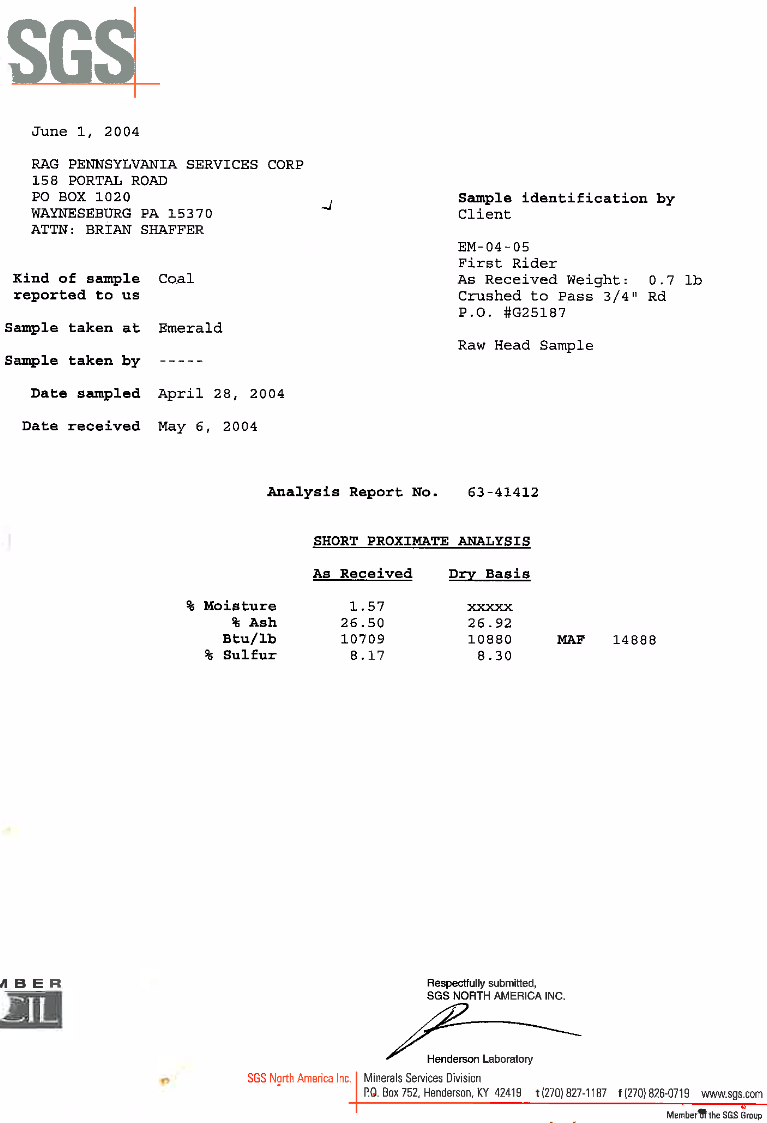
The complete lab report for this hole can be viewed here: Reserve Estimation.pdf [2]
There may be multiple lab reports. The example here focuses on the chemical characteristics of the coal. In many cases, we'll conduct physical tests on the cores to determine geotechnical parameters, e.g. compressive strength, on the ore as well as the rock around the orebody.
We will want to build a database that contains the parameters of interest for each of the holes. If we are interested in determining the average grade, then our table will begin with two columns: drill hole number and the grade for the sample from that hole. Let's suppose that we have a property with 9 holes:
| Hole # | Grade, % |
|---|---|
| 1 | 2 |
| 2 | 3 |
| 3 | 4 |
| 4 | 3 |
| 5 | 4 |
| 6 | 5 |
| 7 | 2 |
| 8 | 3 |
| 9 | 4 |
We want the average grade for the deposit. Is the average grade equal to the arithmetic average, which is 3.33%?
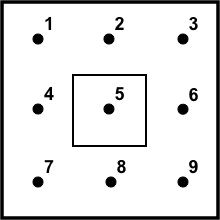
Are the holes spaced uniformly on a grid, like this?
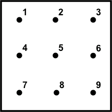
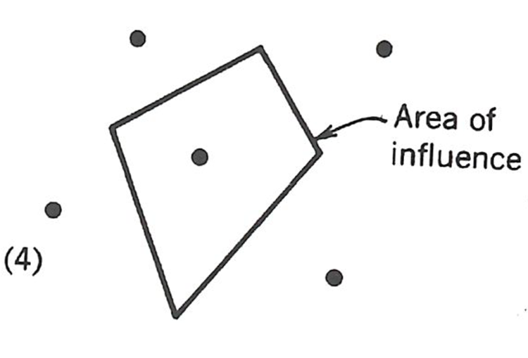
If so, it will be easy to define an area around each hole and then to say that everything within that area has the same properties as those found in the drill hole. Let's draw a box around hole number 5 to illustrate this. Shortly we'll refer to this area as an area of influence.
If the area around each hole were identical, then it would seem reasonable to say that the average grade of this orebody equals the arithmetic average of 3.33%. But wait a minute! We've said nothing about the thickness of the orebody at each hole. Assuming the thickness is identical at each hole, then each hole will represent an identical volume of ore, and computing the arithmetic average yields the correct average grade for the orebody.
However, it's rare that the orebody thickness would be the same at each hole. For the purposes of this example, let's assume a more realistic case in which the thicknesses vary from hole-to-hole. Logically then, a hole through a thicker section of the orebody will represent a greater volume of ore than a hole through a thinner section. If we simply average the two holes together, we will arrive at an incorrect average grade because we have not accounted for the larger contribution of the one hole into the total. We can correct this by using a weighted average, in which the grade of the hole is increased or decreased to reflect the volume that it represents.
3.2.2: The Concept of an Area or Volume of Influence
3.2.2: The Concept of an Area or Volume of Influence
Procedurally, we do this by calculating an area and volume of influence for each hole. The weighted average for the grade, or whatever characteristic is of interest, is obtained by multiplying the value of that characteristic by the volume of influence; and then summing the products and dividing the sum by the sum of the weighted volumes.
Mathematically, this is expressed as:
where = the % grade for the nth hole, and = volume of influence for the nth hole.
Let’s continue with the example by adding the thickness at each hole and inserting columns for the calculated values.The area of influence is the area surrounding each hole, and if the holes are spaced at 400’ intervals, then the area represented by each hole is 1.6x 105ft2.
| Hole # | Area of Influence, ft2 z 103 | Thickness, ft | Volume of Influence, ft3 x 106 | Grade, % | Weighted Grade, %-ft3 x 106 |
|---|---|---|---|---|---|
| 1 | 1600 | 40 | 64 | 2 | 128 |
| 2 | 1600 | 45 | 72 | 3 | 216 |
| 3 | 1600 | 70 | 112 | 4 | 448 |
| 4 | 1600 | 54 | 86.4 | 3 | 259.2 |
| 5 | 1600 | 58 | 92.8 | 4 | 371.2 |
| 6 | 1600 | 70 | 112 | 5 | 560 |
| 7 | 1600 | 42 | 67.2 | 2 | 134.4 |
| 8 | 1600 | 56 | 89.6 | 3 | 268.8 |
| 9 | 1600 | 65 | 104 | 4 | 416 |
| Sum | 14400 | 800 | 2801.6 |
The average grade of the orebody is the weighted grade, 2801 x 106 %-ft3 divided by the volume of influence, 800 x 106 ft3, which equals 3.5%.
Note that the average grade is NOT the arithmetic average of 3.33%. A tenth of a percent error in the grade is quite meaningful. It is important to calculate weighted rather than arithmetic averages in all cases.
In the foregoing example, we had a convenient simplification: the area of influence was the same for each of the holes. In practice, this would rarely be true because the property boundaries are generally irregular and the holes are most likely not spaced evenly. In these common situations, we need a way to determine the influence that a given hole should have in our estimation of the reserve.
Defining an Area or Volume of Influence for a Drill Hole
Consider the following property.

The new challenge here is to determine the area of influence for each hole. Once we have done that, we can continue by using the same procedure that we followed for the previous example.
Each hole is likely to have a different value for the characteristics of interest, and for this discussion let’s say that we are looking at grade. How far from the hole should we assume that the grade of that hole applies? Halfway to an adjacent hole? What if the grade in the adjacent hole is significantly different? Should that alter where we draw the area of influence? Perhaps, we should use a scheme that says the value at the hole decreases inversely as we go further from the hole? In fact, many deterministic and statistical methods have been developed over the years, and some provide better results than others for certain types of ore bodies. Let's take a look at a few methods for determining an area of influence for each drill hole.
3.2.3: Overview of Reserve Estimation Methods
3.2.3: Overview of Reserve Estimation Methods
The polygon method is an old and established approach based on a simple geometric algorithm, in which we construct a polygon around each hole to determine an area of influence for that hole; and then the total volume directly beneath the polygon is assigned the same values as the drill hole from which we constructed the polygon. We’ll take a closer look at his method shortly.
Another method, known as the triangle method, requires that we connect adjacent holes into triangles. The included area of each triangle is assigned the characteristic not of a single hole, but of the weighted average of the three holes forming the triangle. The weighting of the three holes is based on the length of the drill holes.
The inverse distance method is a more complex scheme in which the contribution of a given hole is weighted according to its distance from the block in which the estimate is to be made. The closer a hole is, the more weight is given to its value compared to the values of other holes in the region.
Geostatistical methods employed for ore reserve estimation utilize three-dimensional spatial statistics to improve the quality of the estimate. Classical statistics requires use of a particular distribution model, e.g., the data are normally distributed, and that the samples be independent of one another. Generally, we have insufficient samples of the orebody to assign a distribution, and moreover, the samples are often correlated, i.e., they do not satisfy the independence requirement of classical statistics. Given that the samples, i.e., the drillholes, are limited in number because they are expensive to acquire, often biased, and nearly always smaller in number than is desired, geostatistics is a powerful tool for improving the quality of the estimation.
A prerequisite to a reasonable prediction of the grade of the orebody is a good prediction of the spatial distribution of the grade, or whatever characteristic is of interest. This spatial estimation is accomplished using the sample data and a model known as a variogram, which is used to represent the correlation between the samples. This estimation is often accomplished using a technique known as kriging. Kriging provides an optimal interpolation using the variogram; and the technique is similar to simple interpolation, as we would use in say the inverse distance algorithm, but is different, because it allows us to take into account information that we know about the geology and attendant properties. Based on geologic knowledge of the presence of a certain feature, we will know that the characteristics of all points contained in that feature should be the same or similar. This is an instance where samples are correlated. With geostatistical methods, we can use this knowledge to improve the estimate of grade, or whatever, at points where we have not sampled. The science of geostatistics continues to evolve, becoming more accurate. You will learn the common geostatistical techniques, their strengths, and limitations in MNG 412.
Today, you can enter your exploration data into a computer program and then within minutes, you can have estimates of the resource from several different methods. Then, you will choose which estimate to use. That choice may be based on experience or a heuristic such as selecting the estimate that has the smallest variance. The commercially available mine planning software programs, such as the Carlson software that we use, allow you to employ several different techniques. We are not going to look into these methods in any greater details in this course, with one exception --the polygon method. This method is useful to illustrate the concepts and is a reasonable estimation method in its own right.
The Polygon Method
We begin with a map showing the surface location of the drill holes, and our task is to construct polygons around each hole. The relevant characteristic, say grade, inside of that entire polygon will be the same as the value of that characteristic in the drill hole sample.
We start our work by arbitrarily selecting a drill hole, and then drawing lines between that hole and all the adjacent holes, as shown here.
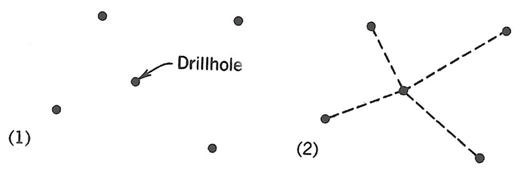
Next, we draw perpendicular bisectors though each of these lines, drawing the bisector line long enough to intersect the other perpendicular bisectors, as shown.
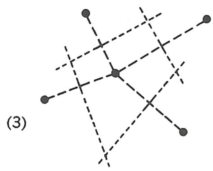
The corners of the polygon are defined by the intersection of the perpendicular bisectors, as shown.
Watch this video (2:59) of a demonstration of using the Polygon Method.
We repeat the process for each hole. Note that if the hole is adjacent to the property boundary, then that boundary line will form a side of the polygon. The result will be a property containing as many polygons as holes, as illustrated here.
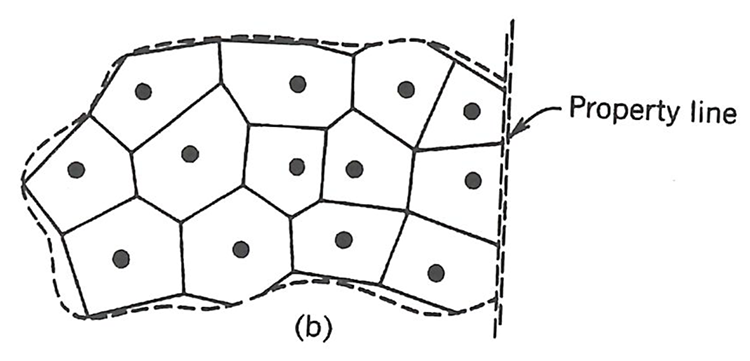
Next, we need to determine the area of each polygon. This can be done manually using a planimeter, or digitally. The result will be an area of influence, i.e., the area of the polygon, for each hole. Then, we can calculate the volume of influence of each polygon, by multiplying the area of influence by the thickness of the ore, or overburden. The next step is to build a table or spreadsheet to facilitate the calculations. We actually did that earlier, in Lesson 3.2.2, and will not repeat it again. At that time, we only calculated the average grade. We could have added any number of other characteristics to the table, and calculated their average value. Examples would include thickness of the deposit and overburden, as well as other characteristics of interest.
3.2.4: Step 2 -- How Much of the Resource is a Reserve?
3.2.4: Step 2 -- How Much of the Resource is a Reserve?
We started this lesson by noting that reserve estimation is completed in two steps. The first is to estimate the size of the resource, which we have now done. The second step is to determine how much of the resource can be mined economically at a point in time.
We’ll need to learn more about mining methods to tackle that question completely, and we will do so in the coming weeks. Notwithstanding, there are two metrics that can be computed very early in this second step. The first metric is known as the cutoff grade, which is basically the lowest grade that can be mined at a profit. The second metric is applicable to shallower deposits that are being evaluated for surface rather than underground mining, and it is known as the stripping ratio. Let’s start with stripping ratios, and let’s use a shallow coal seam for our example.
Stripping Ratios
The coal seam will be underneath layers of soil and rock. The material overlying the seam is known as the overburden. Before we can extract the coal, we first have to remove, i.e., strip, this overburden. It costs money to remove the overburden, and in the simplest terms, the cost of removing the overburden cannot exceed the value of the coal that is exposed.
The stripping ratio is usually taken as the volume of the overburden that must be removed to the weight of the coal that is exposed when this volume of overburden is removed. Thus the units for the stripping ratio will be yd3/ton. Two stripping ratios are used in the prefeasibility or feasibility analyses: overall stripping ratio and the maximum stripping ratio. As mine planning advances beyond the prefeasibility stage, stripping ratios at different cross sections will be calculated as well.
The overall stripping ratio is calculated using the average values for the volume of the overburden and the average value for the weight of the coal (ore). This number is a key indicator for the potential of the project to be profitable. Please remember that these averages are weighted averages.
The maximum stripping ratio, which is also known as the breakeven stripping ratio, is an economic calculation based on the cost of removing the overburden and the value of the coal or ore that is exposed when the overburden is removed. Thus, given the stripping cost and the value of the exposed ore, we can calculate the breakeven or maximum stripping ratio. Stripping costs can be estimated reasonably well, based on the method of overburden removal and the region in which the mining is being conducted. We can find tables of data in handbooks to help us with this estimation. The value of the coal or exposed ore is usually taken to be its selling price. The selling price must account for the mining and processing costs, and the minimum profit that the company requires.
Stripping cost = Value of the exposed coal
where:
- SC = stripping cost, $/yd3
- Vob= volume of overburden that will be removed at breakeven
- Vc= volume of coal that will be exposed by the removal of Vob
- t = thickness of the coal seam
- TF = tonnage factor (density) of the coal, tons/yd3
- SP = selling price of the coal, $/ton
The breakeven or maximum stripping ratio, SRmax, is, therefore:
The value and use of SRmax is illustrated in two examples. Consider the situation represented in the following figure of a coal stripping operation.
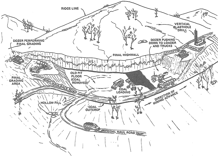
The coal seam is under a hill. Most likely mining started at the edge of the hill where the coal seam outcropped, i.e., intersected the surface. As mining progresses back into the hill, it will be necessary to remove increasing amounts of overburden to expose and mine the coal. At what point does it become uneconomical to remove the overburden to access the coal? Correct –at SRmax! And how do we find SRmax? Correct –using Equation 3.2.3. And therefore, at the point where we are at this maximum stripping ratio, SRmax we will stop mining.
The calculation of stripping ration is slightly more complicated for deposits that are not flat lying, i.e., they are dipping at angle greater than a few degrees; although, conceptually, the process is the same regardless of the spatial characteristics of the deposit. As you'll see, the math is slightly more involved to complete the calculation of the stripping ratio. Let's take a look.
3.2.5: Instantaneous Stripping Ratio
3.2.5: Instantaneous Stripping Ratio
The stripping ratio (SR) refers to the amount of waste material that must be removed for a given amount of ore. The Instantaneous Stripping Ratio (ISR) is the stripping ratio for a given push back, where a tiny slice of material, i.e., ore and/or waste, is removed from a pit wall. This section presents the ISR calculation for a steeply pitching deposit.
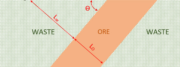
Assume an idealized tabular and steeply pitching orebody that outcrops at the surface and dips to the left at ϴ degrees (Figure 3.2.10). Assume that the ore extends down to considerable depth, and that open-pit mining will be used to extract ore. When open-pit mining is no longer economical, an underground mining method will be used to recover the ore. Therefore, we will need to calculate the point at which we will cease surface mining and either go underground or close the mine.
The over-lying waste, i.e., the non-mineral-bearing rock must be removed to uncover and mine the ore. The shape and size of the pit depends upon economic, engineering, and production factors. Assuming all other factors to be constant, as the selling price of the ore increases, the pit size will increase.
If you were going to calculate the ISR for a “real” orebody for which you had drillhole data, you would utilize one of the computer software packages, such as Carlson. Here the purpose is to teach you the principles, so we are going to make some assumptions to simplify the calculations, and to better illuminate the procedure without getting buried in the math. The assumptions are as follows.
- The seam thickness is constant. The orebody thickness is represented by the length of the ore section (Lo) in the previous diagram. Note that the length of the waste section (Lw) increases as our pit advances deeper. Therefore, as we advance, more of waste will have to be removed to expose a unit of ore, as shown in the next diagram.
- The density of ore and waste are the same.
- All slices have the same strip width (Ws).
- We are looking at a two-diminsional slice of the Earth’s crust. Obviously, the ore and overburden continue into the page and go on for some distance. For our purposes here, we will assume that they go into the page for a distance of 1 unit.
- The slices of the material are mined out perpendicular to the orebody.
Watch this video (3:11) on an explanation of the instantaneous stripping ratio.
Later in this section, I will explain how each of these assumptions affects the calculations. However, it would be instructive for you to pause for a moment and think about each assumption.
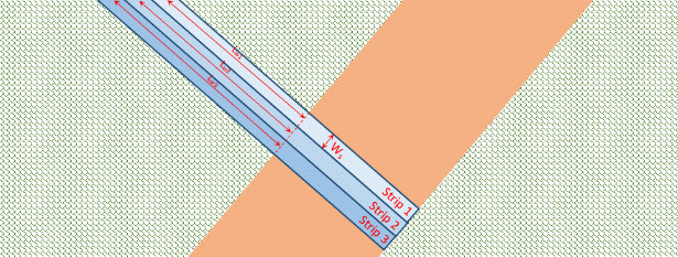
Now, let’s calculate the ISR for strip 1:
where T is strip thickness, L is strip length, W is strip width and is material density.
Since the density, width, and thickness of the ore and waste are assumed to be equal, this equation reduces to:
Assume that the ore seam thickness is 40 ft and the length of the waste slice on top of the ore in strips 1, 2 and 3 is 45, 50 and 55, respectively. The ISR for these three strips is calculated as:
This simplified example has illustrated how the length of waste and ore sections will impact the ISR. In a mine, there will be differences in the density of the ore and waste materials. However, the difference can be trivial in some cases. In fact, a real-world example is where there are several waste types in the slice, and the waste materials have densities that are each different from the ore. Therefore, the calculation of ISR using the length ratio does not work. Instead, a generalized IRS calculation must be defined as:
where there are different waste material types in the strip.
If the density differences are not drastic, the simplified form of the calculation will give you a rough estimate of the ISR. If you need more accurate values with higher accuracy level, then you should consider all other parameters in your calculations. Of course, as I mentioned earlier, if you are doing a complex and “real-world” case, you will probably be using a software package; and then, accounting for the myriad of details becomes easier.
By the way, please note that the ISR is independent of the deposit's dip angle.
For this discussion, we have used an orebody of uniform shape and plunging at some angle θ. But what of a deposit with an irregular shape? The same process applies. Therefore, regardless of the shape of the orebody, the above equation can be used to determine ISR for a strip extracted from the side wall of the pit. It should be also noted that different units can be used to express the ISR.
The most popular units for the ISR are tons of waste removed/ton of ore exposed, ft of waste removed/ft of ore exposed, and yd3 of waste removed/ton of ore exposed. The latter is the most common unit in many types of nonmetal operations because there is no value to know the weight of the waste, unless it poses a limit to the trucks. Therefore, the density of waste material does not come into play in the calculations. If there is an issue with a weight limit in the haul trucks, then the tons of waste/ton of ore is an appropriate unit for the ISR or SR.
3.2.6: Maximum Allowable Stripping Ratio (SRmax)
3.2.6: Maximum Allowable Stripping Ratio (SRmax)
Earlier in this lesson, we looked at the maximum stripping ratio, and we did it for coal seam. You will recall that the maximum allowable stripping ratio, SRmax, also called break-even stripping ratio, is the maximum amount of overburden/waste that can be extracted per unit of ore at the economic pit limit. The SRmax is determined solely by economics, to establish the ultimate boundary of the pit, where break even occurs, i.e. the profit margin is zero. As we defined it before,
So, it is a physical quantity that is determined by economics. This value can be simply converted to the unit of tonsw/tono, considering the density of the waste material. If the ISR exceeds the SRmax , then the operation will be uneconomical as the income generated by the ore will be insufficient to offset the costs incurred in mining.
Now, let’s imagine a massive irregular deposit, where copper ore is the only ore that is desired to be mined out. Unlike coal deposits, metals are not extracted in their native form, except in rare cases. Instead, the rock has a small percentage of valuable minerals in it. A copper deposit contains rock that can be profitably mined and processed to extract the copper. However, the amount of copper contained within the rock, i.e. the grade, varies by location. We’ll need to account for this in our calculation of the break-even stripping ratio.
The only difference is that ore grade variation should be taken into account in the calculation. In order to determine the SRmax for such a deposit, the orebody is divided into different blocks of ore. The average ore grade for each block is determined, and then the overall grade of the ore in the slice is calculated as follows:
where is the average ore grade in the slice, is the length of the ore section that has a grade equal to .
After you calculate the average ore grade for the slice, you can use a grade - stripping ratio (g-SR) plot to determine the SRmax associated with the determined average ore grade. Here is an example of a g-SR plot.
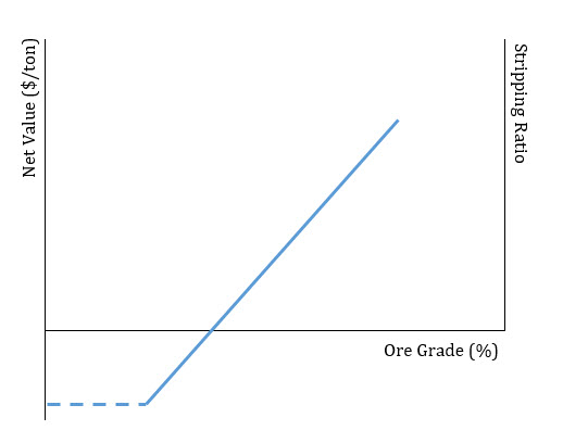
Imagine a copper deposit in which the average copper grade for a strip is 1.05%. Checking the g-SR plot for that deposit, suppose we find out that the SRmax for = 1.05 is equal to 8.5. This means that 8.5 units of waste can be economically removed per unit of ore. If the ISR for the strip is smaller than the SRmax , then the pit could be extended and more strips could be mined profitably. If the ISR and SRmax are equal, then this is a good place for the pit limit. If the ISR is larger than SRmax, then we have passed the economic location for the pit limit.
In MNG 441, you will learn how to determine break-even cutoff grade and draw a g-SR plot using economic parameters. Here, I simply want you to know about this plot and what it is representing.
3.2.7: Impact of Pit Expansion on Stripping Ratio
3.2.7: Impact of Pit Expansion on Stripping Ratio
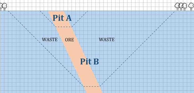
Imagine a steeply pitching orebody, as shown below. We would like to extract this tabular deposit using open pit mining method. Let’s assume that two pits with different sizes are being considered for this mining operation. We would like to study the impact of pit expansion on stripping ratio by comparing the overall stripping ratios for these two pits.
This figure shows the pit areas as a block model. The smaller pit (Pit A) includes 32 blocks. 16 blocks are ore and the other 16 are waste blocks. Therefore, the stripping ratio is 16/16 = 1. The larger pit includes 437 blocks in total. Using Pit 2, 76 blocks of ore can be extracted. Therefore, the stripping ratio is: (437-76)/76 = 4.75. This example shows that as we expand the pit in a steeply pitching orebody, overall stripping ratio dramatically increases. Therefore, more waste blocks have to be mined out to uncover one block of ore. It should be noted that as we go deeper in an open pit, the unit cost of mining will increase. Because the material will be transported for a longer distance, which takes more time, and which may necessitate that we add additional trucks to the fleet.
Now, you should be able to:
- Determine ISR for given pit dimensions
- Find the pit limit when the pit dimensions, average ore grade of the strip and g-SR plot are given.
3.2.8: The Concept of a Cutoff Grade
3.2.8: The Concept of a Cutoff Grade
We know that orebody characteristics such as the grade vary spatially within the orebody, and as we approach the boundaries of the deposit, the grade will begin to decrease to zero. Eventually, the cost to mine and process a ton of ore will exceed the value that we can obtain by selling the commodity found in that ton of ore. Mining companies, like other businesses, do not stay in business by selling their product at a loss!
Thus, when we are estimating the amount of the resource that can be mined economically, we’ll have to calculate a cutoff grade; and any ore with a grade lower than the cutoff cannot be counted in the estimate of the reserve. The cutoff grade is the grade at which the cost of mining and processing the ore is equal to the desired selling price of the commodity extracted from the ore.
The cutoff grade is influenced by a few external factors that you can control to a certain extent, and these will be considered in the prefeasibility analysis when the cutoff grade is determined.
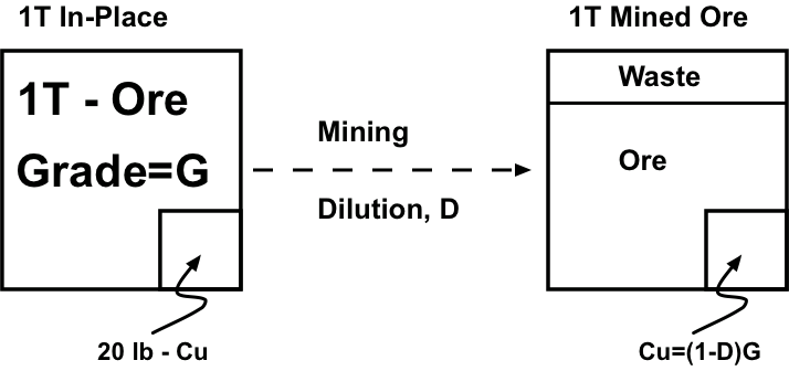
Let’s imagine that we have a deposit of copper that we are evaluating. It is a large resource with a grade of 1%. The block below represents 1 ton (T) of in-place ore. We know that the grade is 1%, so we have 20 lb. of copper distributed in that ton of ore. Let’s represent that 20 pounds of copper as a small (not-to-scale) block inside of the larger block.

When we mine this ton of ore, it is likely that we will get some dilution, which occurs when we extract some of the rock surrounding the orebody. In other words we are diluting our ore with this host rock. Why would we do that? We don’t do it on purpose, generally, but, it is a consequence of the mining method and equipment that we select to mine the ore. Imagine that you have a chocolate cake, and this cake has a thin band of raspberry filling in the middle of the cake. Suppose that you are tasked with removing the raspberry layer, and that you do not want to have any of the chocolate layers mixed with the raspberry layer that you are extracting. Further, I will give you a tiny, baby-sized spoon to complete the task on your cake, and I will give your classmate a large serving-size scoop to complete the task on his cake. You both have ten minutes to complete the job, with a goal of minimizing the dilution of the raspberry layer with the chocolate cake..
The outcome of this experiment is evident. The use of the tiny, rather than large spoon will allow the competitor to be more exacting in the removal of the raspberry layer, resulting in far less contamination, i.e. dilution, of the product. In mining terms, we refer to this as the selectivity of the mining method, and some methods are much more selective than others, resulting in far less dilution. Of course, there are tradeoffs between selectivity and other important metrics such as mining cost and productivity. We’ll look closely at this when we study the mining methods. Now, we can continue with our example.
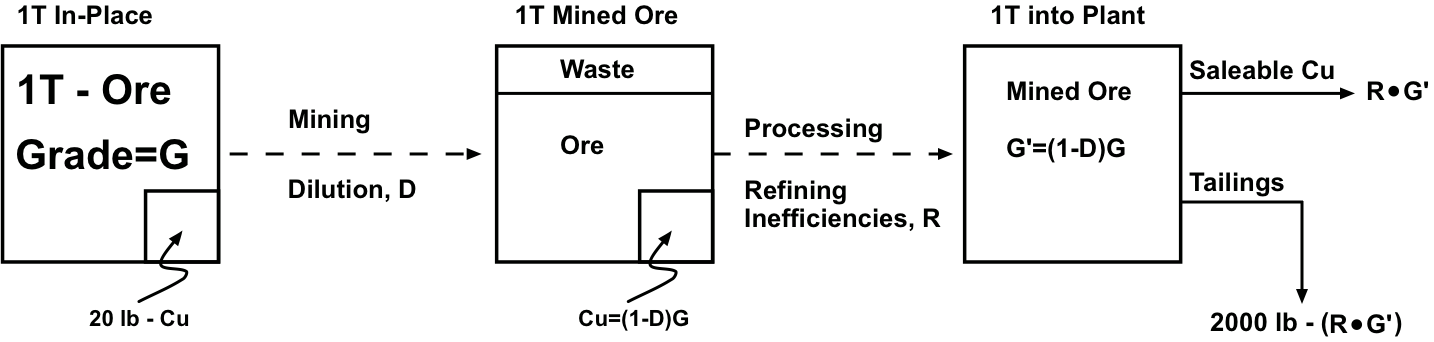
We extract one ton of material, and now we know that this one-ton of material will be diluted with non-ore bearing material, based on how selective our mining method is estimated to be. We can represent this as shown in Figure 3.2.15 by including the waste within the one ton of mined ore. This waste material effectively reduces the copper in the block by the amount of the dilution. Let’s assume an average dilution of 5%. The copper present in the mined block of ore is reduced by 5%, to 19 lb of copper.
Next, our one-ton block of mined material will be routed into the mineral processing plant, where the ore will be separated and concentrated into a saleable product. There will be two output streams from the plant: one containing the saleable product and the other, the tailings, or waste. The physical and chemical methods used to beneficiate the ore are not perfect, and while we can invest more money to improve them, there is a point of diminishing return. Consequently, some saleable product will report to the waste stream, and as such represents a loss. Let’s assume a plant recovery of 90%, meaning that all but 10% of the product in the plant feed will be recovered and report to the product stream. In our example, there is 19 lb. of copper in the feed to the plant and the plant will recover all but 1.9 lb. Thus, the one ton of material that we mined will yield 17.1 lb of copper for sale.
Mathematically, the minimum acceptable grade to mine, i.e. the cutoff grade, occurs when the cost to mine and process the material, (M&P cost), is equal to the value of the product, i.e. its selling price, SP.
We will account for the dilution and recovery losses in the right side of the equation, as these losses are reducing the value of the in-place ore.
where:
- M&P cost = mining & processing cost, $/T
- SP = selling price of the copper, $/lb
- D = dilution
- R = plant recovery
- G = grade
Let’s use some numbers. Assume the following: we have a dilution of 5%, a plant recovery of 92%, a mining and processing cost of $6.80/ton and a selling price of $0.74/lb. Be careful with the units!
Solving the equation for grade, we have:
And substituting our values,
Therefore for this example, the grade of the ore that we choose to mine must have a grade of 0.5% of greater. In other words, the cutoff grade has been determined to be 0.5%, and when you report the size of your reserve, you will include only the tonnage at or greater than 0.5%. Do you understand why you must report it in that way?
Imagine a situation in which your resource contains significant tonnage at slightly less than 0.5%. Likely you will reexamine your dilution and plant recovery assumptions, and explore options for improving both so that you can economically mine the lower grade ore.
We didn’t say much about the selling price itself. Presumable, it is the maximum price that we believe we can reasonably expect to sell our product into the market. The price will need to cover not only our mining and processing costs, but also whatever profit we require. When companies evaluate the merits of opening a new mine they will have certain criteria for establishing the financial merits of the project. They might, for example, require a certain return on their invested capital, a payback within so many years, and so forth. This can all be bundled, at least conceptually, into the required selling price.
Sometimes we will talk about the gross value of the mined ore. The gross value is equal to:
The unit profit is then defined as: Gross Value – Mining & Processing Cost.
To illustrate, assume that we are mining an orebody with a grade of 1.2%, dilution is negligible, and the selling price is $0.74/lb. The gross value is calculated to be $16.34/T and the unit profit is $9.54.