Identification
Digital Line Graphs (DLGs) are vector representations of most of the features and attributes shown on USGS topographic maps. Individual feature set (outlined in the table below) are encoded in separate digital files. DLGs exist at three scales: small (1:2,000,000), intermediate (1:100,000) and large (1:24,000). Large-scale DLGs are produced in tiles that correspond to the 7.5-minute topographic quadrangles from which they were derived.
| Layer | Features |
| Public Land Survey System (PLSS) | Township, range, and section lines |
| Boundaries | State, county, city, and other national and State lands such as forests and parks |
| Transportation | Roads and trails, railroads, pipelines and transmission lines |
| Hydrography | Flowing water, standing water, and wetlands |
| Hypsography | Contours and supplementary spot elevations |
| Non-vegetative features | Glacial moraine, lava, sand, and gravel |
| Survey control and markers | Horizontal and vertical monuments (third order or better) |
| Man-made features | Cultural features, such as building, not collected in other data categories |
| Woods, scrub, orchards, and vineyards | Vegetative surface cover |
Layers and contents of large-scale Digital Line Graph files. Not all layers available for all quadrangles (USGS, 2006).
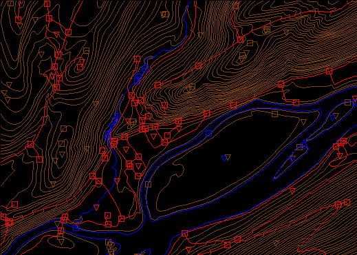
Portion of three Digital Line Graph (DLG) layers for USGS Bushkill, PA quadrangle; imaged with Global Mapper (dlgv32 Pro) software. Transportation features are arbitrarily colored red, hydrography blue, and hypsography brown. The square symbols are nodes and the triangles represent polygon centroids.
Data quality
Like other USGS data products, DLGs conform to National Map Accuracy Standards. In addition, however, DLGs are tested for the logical consistency of the topological relationships among data elements. Similar to the Census Bureau's TIGER/Line, line segments in DLGs must begin and end at point features (nodes), and line segments must be bounded on both sides by area features (polygons).
Spatial Reference Information
DLGs are heterogenous. Some use UTM coordinates, others State Plane Coordinates. Some are based on NAD 27, others on NAD 83. Elevations are referenced either to NGVD 29 or NAVD 88 (USGS, 2006a).
Entities and attributes
The basic elements of DLG files are nodes (positions), line segments that connect two nodes, and areas formed by three or more line segments. Each node, line segment, and area is associated with two-part integer attribute codes. For example, a line segment associated with the attribute code "050 0412" represents a hydrographic feature (050), specifically, a stream (0412).
Distribution
Not all DLG layers are available for all areas at all three scales. Coverage is complete at 1:2,000,000. At the intermediate scale, 1:100,000 (30 minutes by 60 minutes), all hydrography and transportation files are available for the entire U.S., and complete national coverage is planned. At 1:24,000 (7.5 minutes by 7.5 minutes), coverage remains spotty. The files are in the public domain, and can be used for any purpose without restriction.
Large- and Intermediate -scale DLGs are available for download through EarthExplorer system (http://earthexplorer.usgs.gov). You can plot 1:2,000,000 DLGs on-line at the USGS' National Atlas of the United States (http://nationalatlas.gov/).
Digital Line Graph Hypsography
In one sense, DLGs are as much "legacy" data as the out-of-date topographic maps from which they were produced. Still, DLG data serve as primary or secondary sources for several themes in the USGS National Map, including hydrography, boundaries, and transportation. DLG hypsography data are not included in the National Map, however. It is assumed that GIS users can generate elevation contours as needed from DEMs. DLG hypsography and hydrography layers are the preferred sources from which USGS DEMs are produced, however.
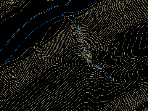
Portion of the hypsography and hydrography layers of a large-scale Digital Line Graph (DLG). USGS Bushkill, PA quadrangle; imaged with Global Mapper (dlgv32 Pro) software.
Hypsography refers to the measurement and depiction of the terrain surface, specifically with contour lines. Several different methods have been used to produce DLG hypsography layers, including:
- Scanning contour lines on photographic film or paper maps, converting the scanned raster data to vectors, then editing and attributing the vector features;
- Manually digitizing and attributing contour lines on photographic film or paper maps; and
- Producing contours by photogrammetric processes.
The preferred method is to manually digitize contour lines in vector mode, then to key-enter the corresponding elevation attribute data.
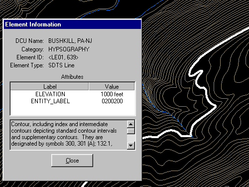
The highlighted contour line has been selected, and its attributes reported in a Global Mapper window. Notice that the line feature is attributed with a unique Element ID code (LE01, 639) and an elevation (1000 feet).
| Try This! |
Exploring DLGs with Global Mapper (dlgv32 Pro)Now I'd like you to use Global Mapper (or dlgv32 Pro) software to investigate the characteristics of the hypsography layer of a USGS Digital Line Graph (DLG). The instructions below assume that you have already installed software on your computer. (If you haven't, return to installation instructions presented earlier in Chapter 6). First you'll download and a sample DLG file. In a following activity you'll have a chance to find and download DLG data for your area.
|