Lesson 7 - Understanding GIS Error, Accuracy, and Precision, and Metadata
An Overview of Lesson 7
The error, accuracy, and precision of the GIS data we use in projects are often overlooked when we download data from various government, open source, and commercial sources. Metadata is data about data. We'll explore these topics in more detail in this lesson.
What will we learn in Lesson 7?
By the end of this lesson, you should be able to:
- explain the requirements for meeting horizontal accuracy;
- apply the accuracy standards for different horizontal scales;
- identify sources of imprecision and error; and
- find and evaluate metadata.
What is due for Lesson 7?
This lesson will take us one week to complete. Please refer to the Calendar for specific time frames and due dates. Specific directions for the assignments below can be found in this lesson.
- Lesson 7 Quiz
- Metadata Activity
- Complete the Esri training course "Editing Basics in ArcGIS Pro"
- Download the following files titled "SAMPLE_ROUTING_PROJECT.zip", "Geography 469 Term Project_Rev_11132018_RAS.docx", "EPRI_GTC_OETL_SITING_METHODOLOGY.pdf", and "Glasgow_White_Paper.pdf" to your Desktop
- Two extra credit opportunities
- Take the anonymous, ungraded mid-course survey
Questions?
If you have any questions, please post them to our Questions? discussion forum. I will check that discussion forum daily to respond. While you are there, feel free to post your own responses if you, too, are able to help out a classmate.
GIS Errors, Accuracy, and Precision
Errors can be injected at many points in a GIS analysis, and one of the largest sources of error is the data collected. Each time a new dataset is used in a GIS analysis, new error possibilities are also introduced. One of the feature benefits of GIS is the ability to use information from many sources, so the need to have an understanding of the quality of the data is extremely important.
Accuracy in GIS is the degree to which information on a map matches real-world values. It is an issue that pertains both to the quality of the data collected and the number of errors contained in a dataset or a map. One everyday example of this sort of error would be if an online advertisement showed a sweater of a certain color and pattern, yet when you received it, the color was slightly off.
Precision refers to the level of measurement and exactness of description in a GIS database. Map precision is similar to decimal precision. Precise location data may measure position to a fraction of a unit (meters, feet, inches, etc.). Precision attribute information may specify the characteristics of features in great detail. As an example of precision, say you try on two pairs of shoes of the same size but different colors. One pair fits as you would expect, but the other pair is too short. Do you suspect a quality issue with the shoes or do you buy the shoes that fit? Would you do the same when selecting GIS data for a project?
The more accurate and precise the data, the higher cost to obtain and store it because it can be very difficult to obtain and will require larger data files. For example, a 1-meter-resolution aerial photograph will cost more to collect (increased equipment resolution) and cost more to store (greater pixel volume) than a 30-meter-resolution aerial photograph.
Highly precise data does not necessarily correlate to highly accurate data nor does highly accurate data imply high precision data. They are two separate and distinct measurements. Relative accuracy and precision, and the inherent error of both precision and accuracy of GIS data determine data quality.
Watch this!
The 11-second video below, created by Glenn Johnson from Penn State's Dutton e-Education Institute, demonstrates the difference between precision and accuracy.
There are 4 archery targets with 4 arrows landing in different places. Where the arrows land demonstrates the archers level of accuracy and precision.
Accuracy and Precision: All arrows land in the bull's eye.
Accuracy and Imprecision: All arrows land on the target in all different places but none on the bull's eye.
Inaccuracy and Precision: All the arrows land in the same area but it is not in the bull's eye.
Inaccuracy and Imprecision: Two arrows hit the target outside of the bull's eye. Two arrows miss the target altogether.
More About GIS Error, Accuracy, and Precision
Let's go into more detail about error, accuracy, and precision. The following information is taken, with permission, from The Geographer's Craft:
1. The Importance of Error, Accuracy, and Precision
Until quite recently, people involved in developing and using GIS paid little attention to the problems caused by error, inaccuracy, and imprecision in spatial datasets. Certainly, there was an awareness that all data suffers from inaccuracy and imprecision, but the effects on GIS problems and solutions was not considered in great detail. Major introductions to the field such as C. Dana Tomlin's Geographic Information Systems and Cartographic Modeling (1990), Jeffrey Star and John Estes's Geographic Information Systems: An Introduction (1990), and Keith Clarke's Analytical and Computer Cartography (1990) barely mention the issue.
This situation has changed substantially in recent years. It is now generally recognized that error, inaccuracy, and imprecision can "make or break" many types of GIS projects. That is, errors left unchecked can make the results of a GIS analysis almost worthless.
The irony is that the problem of error is it devolves from one of the greatest strengths of GIS. GIS gain much of their power from being able to collate and cross-reference many types of data by location. They are particularly useful because they can integrate many discrete datasets within a single system. Unfortunately, every time a new dataset is imported, the GIS also inherits its errors. These may combine and mix with the errors already in the database in unpredictable ways.
One of the first thorough discussions of the problems and sources of error appeared in P.A. Burrough's Principles of Geographical Information Systems for Land Resources Assessment (1986). Now, the issue is addressed in many introductory texts on GIS.
The key point is that even though error can disrupt GIS analyses, there are ways to keep error to a minimum through careful planning and methods for estimating its effects on GIS solutions. Awareness of the problem of errors has also had the useful benefit of making GIS practitioners more sensitive to potential limitations of GIS to reach impossibly accurate and precise solutions.
2. Some Basic Definitions
It is important to distinguish from the start a difference between accuracy and precision:
2.1 Accuracy is the degree to which information on a map or in a digital database matches true or accepted values. Accuracy is an issue pertaining to the quality of data and the number of errors contained in a dataset or map. In discussing a GIS database, it is possible to consider horizontal and vertical accuracy with respect to geographic position, as well as attribute, conceptual, and logical accuracy.
- The level of accuracy required for particular applications varies greatly.
- Highly accurate data can be very difficult and costly to produce and compile.
2.2 Precision refers to the level of measurement and exactness of description in a GIS database. Precise locational data may measure position to a fraction of a unit. Precise attribute information may specify the characteristics of features in great detail. It is important to realize, however, that precise data – no matter how carefully measured – may be inaccurate. Surveyors may make mistakes or data may be entered into the database incorrectly.
- The level of precision required for particular applications varies greatly. Engineering projects such as road and utility construction require very precise information measured to the millimeter or tenth of an inch. Demographic analyses of marketing or electoral trends can often make do with less, say to the closest zip code or precinct boundary.
- Highly precise data can be very difficult and costly to collect. Carefully surveyed locations needed by utility companies to record the locations of pumps, wires, pipes and transformers cost $5-20 per point to collect.
High precision does not indicate high accuracy nor does high accuracy imply high precision. But high accuracy and high precision are both expensive.
Be aware also that GIS practitioners are not always consistent in their use of these terms. Sometimes the terms are used almost interchangeably and this should be guarded against.
Two additional terms are used as well:
- Data quality refers to the relative accuracy and precision of a particular GIS database. These facts are often documented in data quality reports.
- Error encompasses both the imprecision of data and its inaccuracies.
3. Types of Error
Positional error is often of great concern in GIS, but error can actually affect many different characteristics of the information stored in a database.
3.1. Positional accuracy and precision
This applies to both horizontal and vertical positions.
Accuracy and precision are a function of the scale at which a map (paper or digital) was created. The mapping standards employed by the United States Geological Survey specify that:
"requirements for meeting horizontal accuracy as 90 percent of all measurable points must be within 1/30th of an inch for maps at a scale of 1:20,000 or larger, and 1/50th of an inch for maps at scales smaller than 1:20,000."
Accuracy Standards for Various Scale Maps
1:2,400 ± 6.67 feet
1:4,800 ± 13.33 feet
1:10,000 ± 27.78 feet
1:12,000 ± 33.33 feet
1:24,000 ± 40.00 feet
1:63,360 ± 105.60 feet
1:100,000 ± 166.67 feet
1:1,200 ± 3.33 feet
This means that when we see a point on a map we have its "probable" location within a certain area. The same applies to lines.
Beware of the dangers of false accuracy and false precision, that is reading locational information from map to levels of accuracy and precision beyond which they were created. This is a very great danger in computer systems that allow users to pan and zoom at will to an infinite number of scales. Accuracy and precision are tied to the original map scale and do not change even if the user zooms in and out. Zooming in and out can, however, mislead the user into believing – falsely – that the accuracy and precision have improved.
3.2. Attribute accuracy and precision
The non-spatial data linked to location may also be inaccurate or imprecise. Inaccuracies may result from mistakes of many sorts. Non-spatial data can also vary greatly in precision. Precise attribute information describes phenomena in great detail. For example, a precise description of a person living at a particular address might include gender, age, income, occupation, level of education, and many other characteristics. An imprecise description might include just income, or just gender.
3.3. Conceptual accuracy and precision
GIS depend upon the abstraction and classification of real-world phenomena. The users determines what amount of information is used and how it is classified into appropriate categories. Sometimes users may use inappropriate categories or misclassify information. For example, classifying cities by voting behavior would probably be an ineffective way to study fertility patterns. Failing to classify power lines by voltage would limit the effectiveness of a GIS designed to manage an electric utilities infrastructure. Even if the correct categories are employed, data may be misclassified. A study of drainage systems may involve classifying streams and rivers by "order," that is where a particular drainage channel fits within the overall tributary network. Individual channels may be misclassified if tributaries are miscounted. Yet, some studies might not require such a precise categorization of stream order at all. All they may need is the location and names of all stream and rivers, regardless of order.
3.4 Logical accuracy and precision
Information stored in a database can be employed illogically. For example, permission might be given to build a residential subdivision on a floodplain unless the user compares the proposed plan with floodplain maps. Then again, building may be possible on some portions of a floodplain but the user will not know unless variations in flood potential have also been recorded and are used in the comparison. The point is that information stored in a GIS database must be used and compared carefully if it is to yield useful results. GIS systems are typically unable to warn the user if inappropriate comparisons are being made or if data are being used incorrectly. Some rules for use can be incorporated in GIS designed as "expert systems," but developers still need to make sure that the rules employed match the characteristics of the real-world phenomena they are modeling.
Finally, It would be a mistake to believe that highly accurate and highly precision information is needed for every GIS application. The need for accuracy and precision will vary radically depending on the type of information coded and the level of measurement needed for a particular application. The user must determine what will work. Excessive accuracy and precision is not only costly but can cause considerable error in details.
4. Sources of Inaccuracy and Imprecision
There are many sources of error that may affect the quality of a GIS dataset. Some are quite obvious, but others can be difficult to discern. Few of these will be automatically identified by the GIS itself. It is the user's responsibility to prevent them. Particular care should be devoted to checking for errors because GIS are quite capable of lulling the user into a false sense of accuracy and precision unwarranted by the data available. For example, smooth changes in boundaries, contour lines, and the stepped changes of chloropleth maps are "elegant misrepresentations" of reality. In fact, these features are often "vague, gradual, or fuzzy" (Burrough 1986). There is an inherent imprecision in cartography that begins with the projection process and its necessary distortion of some of the data (Koeln and others 1994), an imprecision that may continue throughout the GIS process. Recognition of error and importantly what level of error is tolerable and affordable must be acknowledged and accounted for by GIS users.
Burrough (1986) divides sources of error into three main categories:
- Obvious sources of error.
- Errors resulting from natural variations or from original measurements.
- Errors arising through processing.
Generally errors of the first two types are easier to detect than those of the third because errors arising through processing can be quite subtle and may be difficult to identify. Burrough further divided these main groups into several subcategories.
4.1 Obvious Sources of Error
4.1.1. Age of data
Data sources may simply be to old to be useful or relevant to current GIS projects. Past collection standards may be unknown, non-existent, or not currently acceptable. For instance, John Wesley Powell's nineteenth century survey data of the Grand Canyon lacks the precision of data that can be developed and used today. Additionally, much of the information base may have subsequently changed through erosion, deposition, and other geomorphic processes. Despite the power of GIS, reliance on old data may unknowingly skew, bias, or negate results.
4.1.2. Areal Cover
Data on a give area may be completely lacking, or only partial levels of information may be available for use in a GIS project. For example, vegetation or soils maps may be incomplete at borders and transition zones and fail to accurately portray reality. Another example is the lack of remote sensing data in certain parts of the world due to almost continuous cloud cover. Uniform, accurate coverage may not be available, and the user must decide what level of generalization is necessary, or whether further collection of data is required.
4.1.3. Map Scale
The ability to show detail in a map is determined by its scale. A map with a scale of 1:1000 can illustrate much finer points of data than a smaller scale map of 1:250000. Scale restricts type, quantity, and quality of data (Star and Estes 1990). One must match the appropriate scale to the level of detail required in the project. Enlarging a small scale map does not increase its level of accuracy or detail.
4.1.4. Density of Observations
The number of observations within an area is a guide to data reliability and should be known by the map user. An insufficient number of observations may not provide the level of resolution required to adequately perform spatial analysis and determine the patterns GIS projects seek to resolve or define. A case in point, if the contour line interval on a map is 40 feet, resolution below this level is not accurately possible. Lines on a map are a generalization based on the interval of recorded data, thus the closer the sampling interval, the more accurate the portrayed data.
4.1.5. Relevance
Quite often the desired data regarding a site or area may not exist, and "surrogate" data may have to be used instead. A valid relationship must exist between the surrogate and the phenomenon it is used to study but, even then, error may creep in because the phenomenon is not being measured directly. A local example of the use of surrogate data are habitat studies of the golden-cheeked warblers in the Hill Country. It is very costly (and disturbing to the birds) to inventory these habitats through direct field observation. But the warblers prefer to live in stands of old growth cedar Juniperus ashei. These stands can be identified from aerial photographs. The density of Juniperus ashei can be used as surrogate measure of the density of warbler habitat. But, of course, some areas of cedar may uninhabited or inhibited to a very high density. These areas will be missed when aerial photographs are used to tabulate habitats.
Another example of surrogate data are electronic signals from remote sensing that are use to estimate vegetation cover, soil types, erosion susceptibility, and many other characteristics. The data is being obtained by an indirect method. Sensors on the satellite do not "see" trees, but only certain digital signatures typical of trees and vegetation. Sometimes these signatures are recorded by satellites even when trees and vegetation are not present (false positives) or not recorded when trees and vegetation are present (false negatives). Due to cost of gathering on site information, surrogate data is often substituted, and the user must understand variations may occur, and although assumptions may be valid, they may not necessarily be accurate.
4.1.6. Format
Methods of formatting digital information for transmission, storage, and processing may introduce error in the data. Conversion of scale, projection, changing from raster to vector format, and resolution size of pixels are examples of possible areas for format error. Expediency and cost often require data reformation to the "lowest common denominator" for transmission and use by multiple GIS. Multiple conversions from one format to another may create a ratchet effect similar to making copies of copies on a photo copy machine. Additionally, international standards for cartographic data transmission, storage and retrieval are not fully implemented.
4.1.7. Accessibility
Accessibility to data is not equal. What is open and readily available in one country may be restricted, classified, or unobtainable in another. Prior to the break-up of the former Soviet Union, a common highway map that is taken for granted in this country was considered classified information and unobtainable to most people. Military restrictions, inter-agency rivalry, privacy laws, and economic factors may restrict data availability or the level of accuracy in the data.
4.1.8. Cost
Extensive and reliable data is often quite expensive to obtain or convert. Initiating new collection of data may be too expensive for the benefits gained in a particular GIS project and project managers must balance their desire for accuracy the cost of the information. True accuracy is expensive and may be unaffordable.
4.2. Errors Resulting from Natural Variation or from Original Measurements
Although these error sources may not be as obvious, careful checking will reveal their influence on the project data.
4.2.1. Positional accuracy
Positional accuracy is a measurement of the variance of map features and the true position of the attribute (Antenucci and others 1991, p. 102). It is dependent on the type of data being used or observed. Mapmakers can accurately place well-defined objects and features such as roads, buildings, boundary lines, and discrete topographical units on maps and in digital systems, whereas less discrete boundaries such as vegetation or soil type may reflect the estimates of the cartographer. Climate, biomes, relief, soil type, drainage, and other features lack sharp boundaries in nature and are subject to interpretation. Faulty or biased field work, map digitizing errors and conversion, and scanning errors can all result in inaccurate maps for GIS projects.
4.2.2. Accuracy of content
Maps must be correct and free from bias. Qualitative accuracy refers to the correct labeling and presence of specific features. For example, a pine forest may be incorrectly labeled as a spruce forest, thereby introducing error that may not be known or noticeable to the map or data user. Certain features may be omitted from the map or spatial database through oversight, or by design.
Other errors in quantitative accuracy may occur from faulty instrument calibration used to measure specific features such as altitude, soil or water pH, or atmospheric gases. Mistakes made in the field or laboratory may be undetectable in the GIS project unless the user has conflicting or corroborating information available.
4.2.3. Sources of variation in data
Variations in data may be due to measurement error introduced by faulty observation, biased observers, or by miscalibrated or inappropriate equipment. For example, one can not expect sub-meter accuracy with a hand-held, non-differential GPS receiver. Likewise, an incorrectly calibrated dissolved oxygen meter would produce incorrect values of oxygen concentration in a stream.
There may also be a natural variation in data being collected, a variation that may not be detected during collection. As an example, salinity in Texas bays and estuaries varies during the year and is dependent upon freshwater influx and evaporation. If one was not aware of this natural variation, incorrect assumptions and decisions could be made, and significant error introduced into the GIS project. In any case, if the errors do not lead to unexpected results, their detection may be extremely difficult.
4.3. Errors Arising Through Processing
Processing errors are the most difficult to detect by GIS users and must be specifically looked for and require knowledge of the information and the systems used to process it. These are subtle errors that occur in several ways, and are therefore potentially more insidious, particularly because they can occur in multiple sets of data being manipulated in a GIS project.
4.3.1. Numerical Errors
Different computers may not have the same capability to perform complex mathematical operations and may produce significantly different results for the same problem. Burrough (1990) cites an example in number squaring that produced 1200% difference. Computer processing errors occur in rounding off operations and are subject to the inherent limits of number manipulation by the processor. Another source of error may from faulty processors, such as the recent mathematical problem identified in Intel's Pentium (tm) chip. In certain calculations, the chip would yield the wrong answer.
A major challenge is the accurate conversion of existing to maps to digital form (Muehrcke 1986). Because computers must manipulate data in a digital format, numerical errors in processing can lead to inaccurate results. In any case, numerical processing errors are extremely difficult to detect, and perhaps assume a sophistication not present in most GIS workers or project managers.
4.3.2. Errors in Topological Analysis
Logic errors may cause incorrect manipulation of data and topological analyses (Star and Estes 1990). One must recognize that data is not uniform and is subject to variation. Overlaying multiple layers of maps can result in problems such as Slivers, Overshoots, and Dangles. Variation in accuracy between different map layers may be obscured during processing leading to the creation of "virtual data which may be difficult to detect from real data" (Sample 1994).
4.3.3. Classification and Generalization Problems
For the human mind to comprehend vast amounts of data, it must be classified, and in some cases generalized, to be understandable. According to Burrough (1986, pp. 137), about seven divisions of data is ideal and may be retained in human short-term memory. Defining class intervals is another problem area. For instance, defining a cause of death in males between 18-25 years old would probably be significantly different in a class interval of 18-40 years old. Data is most accurately displayed and manipulated in small multiples. Defining a reasonable multiple and asking the question "compared to what" is critical (Tufte 1990, pp. 67-79). Classification and generalization of attributes used in GIS are subject to interpolation error and may introduce irregularities in the data that is hard to detect.
4.3.4. Digitizing and Geocoding Errors
Processing errors occur during other phases of data manipulation such as digitizing and geocoding, overlay and boundary intersections, and errors from rasterizing a vector map. Physiological errors of the operator by involuntary muscle contractions may result in spikes, switchbacks, polygonal knots, and loops. Errors associated with damaged source maps, operator error while digitizing, and bias can be checked by comparing original maps with digitized versions. Other errors are more elusive.
5. The Problems of Propagation and Cascading
This discussion focused to this point on errors that may be present in single sets of data. GIS usually depend on comparisons of many sets of data. This schematic diagram shows how a variety of discrete datasets may have to be combined and compared to solve a resource analysis problem. It is unlikely that the information contained in each layer is of equal accuracy and precision. Errors may also have been made compiling the information. If this is the case, the solution to the GIS problem may itself be inaccurate, imprecise, or erroneous.
The point is that inaccuracy, imprecision, and error may be compounded in GIS that employs many data sources. There are two ways in which this compounded my occur.
5.1. Propagation
Propagation occurs when one error leads to another. For example, if a map registration point has been mis-digitized in one coverage and is then used to register the second coverage, the second coverage will propagate the first mistake. In this way, a single error may lead to others and spread until it corrupts data throughout the entire GIS project. To avoid this problem, use the largest scale map to register your points.
Often propagation occurs in an additive fashion, as when maps of different accuracy are collated.
5.2. Cascading
Cascading means that erroneous, imprecise, and inaccurate information will skew a GIS solution when information is combined selectively into new layers and coverages. In a sense, cascading occurs when errors are allowed to propagate unchecked from layer to layer repeatedly.
The effects of cascading can be very difficult to predict. They may be additive or multiplicative and can vary depending on how information is combined, that is from situation to situation. Because cascading can have such unpredictable effects, it is important to test for its influence on a given GIS solution. This is done by calibrating a GIS database using techniques such as sensitivity analysis. Sensitivity analysis allows the users to gauge how and how much errors will affect solutions. Calibration and sensitivity analysis are discussed in Managing Error.
It is also important to realize that propagation and cascading may affect horizontal, vertical, attribute, conceptual, and logical accuracy and precision.
6. Beware of False Precision and False Accuracy!
GIS users are not always aware of the difficult problems caused by error, inaccuracy, and imprecision. They often fall prey to False Precision and False Accuracy, that is they report their findings to a level of precision or accuracy that is impossible to achieve with their source materials. If locations on a GIS coverage are only measured within a hundred feet of their true position, it makes no sense to report predicted locations in a solution to a tenth of a foot. That is, just because computers can store numeric figures down many decimal places does not mean that all those decimal places are "significant." It is important for GIS solutions to be reported honestly, and only to the level of accuracy and precision they can support.
This means in practice that GIS solutions are often best reported as ranges or ranking, or presented within statistical confidence intervals. These issues are addressed in the module, Managing Error.
7. The Dangers of Undocumented Data
Given these issues, it is easy to understand the dangers of using undocumented data in a GIS project. Unless the user has a clear idea of the accuracy and precision of a dataset, mixing this data into a GIS can be very risky. Data that you have prepared carefully may be disrupted by mistakes someone else made. This brings up three important issues.
7.1. Ask or look for metadata or data quality reports when you borrow or purchase data
Many major governmental and commercial data producers work to well-established standards of accuracy and precision that are available publicly in printed or digital form. These documents will tell you exactly how maps and datasets were compiled and such reports should be studied carefully. Data quality reports are usually provided with datasets obtained from local and state government agencies or from private suppliers.
7.2. Prepare a Data Quality Report for datasets you create
Your data will not be valuable to others unless you too prepare a data quality report. Even if you do not plan to share your data with others, you should prepare a report – just in case you use the dataset again in the future. If you do not document the dataset when you create it, you may end up wasting time later having to check it a second time. Use the data quality reports found above as models for documenting your dataset.
7.3. In the absence of a Data Quality Report, ask questions about undocumented data before you use it
- What is the age of the data?
- Where did it come from?
- In what medium was it originally produced?
- What is the areal coverage of the data?
- To what map scale was the data digitized?
- What projection, coordinate system, and datum were used in maps?
- What was the density of observations used for its compilation?
- How accurate are positional and attribute features?
- Does the data seem logical and consistent?
- Do cartographic representations look "clean?"
- Is the data relevant to the project at hand?
- In what format is the data kept?
- How was the data checked?
- Why was the data compiled?
- What is the reliability of the provider?
These materials were developed by Kenneth E. Foote and Donald J. Huebner, Department of Geography, University of Texas at Austin, 1995. These materials may be used for study, research, and education in not-for-profit applications. If you link to or cite these materials, please credit the authors, Kenneth E. Foote and Donald J. Huebner, The Geographer's Craft Project, Department of Geography, The University of Colorado at Boulder. These materials may not be copied to or issued from another Web server without the authors' express permission. Copyright © 2000 All commercial rights are reserved. If you have comments or suggestions, please contact the author or Kenneth E. Foote at ken.foote@uconn.edu.
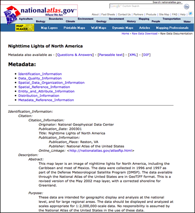
Metadata
What is Metadata?
Metadata is data about data. It is a summary document providing content, quality, type, creation, and spatial information about a dataset. Let’s take an example. You visit a car dealership to purchase a car. On the window of each car is a sticker giving you very specific information about the vehicle including manufacturer, make, model, size of engine, transmission type, miles per gallon, accessories, etc. This is metadata about the characteristics of a specific vehicle. It is the information you use to make an informed decision when comparing and purchasing a vehicle. Without this information, you know nothing about the vehicle and your decision to purchase becomes confusing at best. This is also true for GIS data. If you don’t know what it represents, what it covers, who made it or what quality it is, then only the originator of the data would be able to find and use it. If you do find it and use it, it may be totally inappropriate for your project and give you erroneous results.
Metadata can make clear to users the quality of a dataset or service and what it contains. Based on the metadata, you can then decide whether a dataset or service is useful or not, or whether you need to collect additional data. If the data has a metadata file, the knowledge about the data and services does not disappear if the originator of the data is no longer associated with the data.
It is not necessary for metadata to always give access to the dataset or service; however, it must always indicate where the dataset or service can be obtained.
Official standards organizations define metadata standards. By adhering to common metadata standards, organizations can readily share data. Two organizations set metadata standards. They are the International Organization for Standardization (ISO), and, in the United States, the Federal Geographic Information Committee (FGDC). The FGDC first published the Content Standard for Digital Geospatial Metadata in 1998, and it is the standard used by governmental agencies in the United States.
Where is Metadata found?
OK, so now you know something about metadata, where do you find it? Let’s look at an example.
Try this!
- Navigate to U.S. Department of Agriculture Geospatial Data Gateway where you can obtain soils data for a specific state and county.
- At the landing page, click on the large green DATA button at the top right of the page.
- This brings you to a screen where you should see five tabs in the left sidebar.
- Click on 1-Where Tab. In the center panel, enter your state and county (move county to right pane using>>), then click 'Submit Selected Counties'.
- This takes you to 2-What: Scroll down the center pane until you come to 'Soils', Check the box next to US General Soils Map (STATSGO2), then click 'Continue'.
- You are now on 3-How: Click on 'Continue'.
- You are now on 4-Who: Complete the form and click on 'Continue'.
- You are now on 5-Review: Review the information and click on ' PLACE ORDER' in left sidebar.
- Your data will now be emailed to the address you included on the order form.
- Open the email, look for Ordered Items and click on the link having a .zip file.
- Navigate to where this file has been downloaded to and extract it.
- I believe you will have a file named 'Soils'. There may be a second file to extract. If so, extract this to the 'Soils' file.
- Open the soils file again, and click on a file that has the state abbreviation followed by the date in parentheses (Example: wss_gsmsoil_NC_[2006-07-06])
- Open the soil_metadata_us.txt file.
- What you will see next is the metadata for the specific county soils data you selected. You will now see the metadata including: Identification Information, Data Quality Information, Spatial Data Organization Information, Spatial Reference Information, Entity and Attribute Information, Distribution Information, and Metadata Reference Information. Explore each of these links and familiarize yourself with the information in the various categories. You will get an opportunity to practice using metadata in the class activity that follows.
Metadata Assignment
Activity
In this activity, you will explore metadata further by reviewing actual metadata sets and answering a set of questions about them.
Note
For this assignment, you will need to record your work in a word processing document. Your work must be submitted in Word (.doc) or PDF (.pdf) format so I can open it. In addition, documents must be double-spaced and typed in 12-point Times Roman font.
Directions
- Access the following metadata sets:
- Hydrology (watersheds, subwatersheds, river & streams)
- Digital Ortho Quads
- Watershed Drinking Water Data - Mecklenburg County, NC (Click the DATA Tab > in search box type: Storm Water Watersheds > Click: Metadata).
- For each dataset, answer the following questions in a word processing document. If you cannot find the answer within the metadata, state that as your response:
- What agency or organization created the data?
- When was the data created?
- What is the GIS format (raster or vector)?
- What is the resolution of the data?
- If raster, report cell size
- If vector, report scale
- What is the spatial reference of the data?
- Coordinate system (Geographic, UTM, State Plane, etc.)?
- Projection (Unprojected, Transverse Mercator, Albers Equal Area, etc.)?
- Datum (WGS84, NAD83, NAD27, etc.)?
- How was the original data created (scanned maps, satellite, survey, etc.)?
- What time period does the data cover?
- What data attributes are used?
- What is the unit of the attribute?
- Was all of the data needed to answer the questions readily available?
- How would you rate the data quality of the dataset on a scale of 1 to 5, with 1 = poor data quality and 5 = excellent data quality?
- At the end of your word processing document, respond to the following question:
- What did you learn about metadata from doing this activity?
- Save your work as either a Microsoft Word or PDF file in the following format:
Lesson2_Metadata_AccessAccountID_LastName.doc (or .pdf).
Submitting your work
Submit your work to the Lesson 7 - Metadata drop box by the due date indicated on our course calendar.
Grading Criteria
This activity is graded out of 5 points
| CRITERIA | 8 | 6 | 4 | 2 | 0 |
|---|---|---|---|---|---|
| Dataset Questions | Fully answered all 11 questions for all 4 datasets | Fully answered all 11 questions for 3 of the 4 datasets | Fully answered all 11 questions for 2 of the 4 datasets | Fully answered all 11 questions for 1 of the 4 datasets | Did not fully answer the 11 questions for any of the datasets |
| Answer to Item #3? | n/a | n/a | n/a | Provided written response to Item #3 questions | No written response to Item #3 is provided |
Activity: Editing Basics in ArcGIS Pro
For this activity, you will be completing the Esri tutorial: Editing Basics in ArcGIS Pro. This tutorial will teach you editing basics and work flows. You want to be confident that your data is up to date and accurate. ArcGIS Pro provides editing tools that allow you to update existing features or create new features. Using editing functionality in ArcGIS Pro, you can change the geometry of features or the informational attributes.
Learning Objectives
After completing this course (Esri tutorial: Editing Basics in ArcGIS Pro), you will be able to perform the following tasks:
- create new features and attributes;
- use tools to modify existing features and attributes;
- access and complete the tutorial;
- go to the Esri Academy (www.esri.com/training/) and log in with your Esri username and password to go to the Esri Training page;
- use the search function to search for the course “Editing Basics in ArcGIS Pro”;
- select the “Editing Basics in ArcGIS Pro” course from the list to begin;
- follow the course outline on the left sidebar to navigate and complete the course;
- print or save a copy of the Certificate of Completion to a place where you can easily locate it.
Activity Part 2: Quiz
After you have completed the training course, complete the "Introduction to ArcGIS Reflection Quiz".
Deliverables
Submit your Certificate of Completion to the Lesson 7: Editing Basics in ArcGIS Pro drop box by the due date indicated on the course calendar.
Grading Criteria
This activity will be graded on a simple pass/fail basis but it is worth a full 10% of your course grade. You will "pass" by submitting your Certificate of Completion!
Download Activity
In this activity, we are going to download a dataset that you will use in Lesson 9. You need to complete this task now so that you are ready to jump in and get started on the Lesson 9 Term Project on the first day of Lesson 9. You will be asked to provide a screenshot of your successfully downloaded file as proof.
Directions
Caution
- This activity requires you to pay close attention to detail and follow the instructions completely. Failure to do so can result in extreme frustration.
- The following steps require you to have a C:\temp folder and to unzip files. If you are unsure how to do either of those, watch the Downloading the Term Project Files video in the Term Project Module before getting started.
1. Installing the sample routing project files on your own computer
- Verify your computer has a "C:\temp folder", If not create one.
- Copy the file titled "SAMPLE_ROUTING_PROJECT.zip" to your Desktop or to your Downloads folder on your PC/Laptop. The file is located in the "Term Project Materials" folder.
- To download the file to your own computer, right-click the location link and select "Save Target As" or "Save Link As" from the pop-up menu.
- Once the zipped file is downloaded to your computer, double-click on the downloaded zip file to decompress it to your C:\temp folder. You should end up with a folder called C:\temp\SAMPLE_ROUTING_PROJECT.
Note
THE "SAMPLE_ROUTING_PROJECT" FOLDER SHOULD BE UNZIPPED TO THE C:\temp folder. The siting model may not execute if saved to some other location.
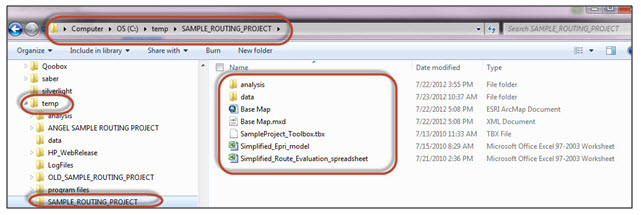
- Verify that the "SAMPLE_ROUTING_PROJECT" folder created in your C:\temp folder (C:\temp\SAMPLE_ROUTING_PROJECT\) contains the following folders/files:
- Analysis folder
- Data folder
- Base_Map.mxd (Esri Map Document)
- SampleProject_Toolbox_v3.tbx
- Simplified_Epri_model.xls
- Simplified_Route_Evaluation_spreadsheet.xls
- Take a screenshot that shows evidence you have successfully completed the download. It should look similar to the one below:
- Save your screenshot using the following naming convention:
L7_download_AccessAccountID_LastName
For example, student Elvis Aaron Presley's file would be named "L7_download_eap1_presley"—this naming convention is important, as it will help me make sure I match each submission up with the right student!
2. Installing transmission line siting exercise for use on a Penn State computer lab computer
If you plan to use a Penn State Computer Lab, follow this link to Additional Instructions for Penn State Computer Labs
Having Problems?
If you are having problems, please consult the FAQ for answers to some of the most frequently asked questions. If that doesn't help, post your questions to the Lesson 7 Discussion Forum.
Submitting Your Work
Upload your screenshot to the "Lesson 7 - Download Screenshot" drop box by the due date indicated on our calendar.
Grading Criteria
The grading for this is slightly different from other assignments. Successful and timely completion of this activity will be reflected in your Lesson 9 grade. The grading will be as follows:
- Completed on time (by end of Lesson 7, see Calendar for details): You will receive two (2) extra points for your Lesson 9 activity. This is the equivalent of half a letter grade for the Lesson 9 activity.
- Completed one (1) to three (3) days late: You will lose 2 points which is the equivalent of half a letter grade for the Lesson 9 activity.
- Completed four (4) or more days late: You will lose 4 points which is the equivalent of a whole letter grade for the Lesson 9 activity.
Summary and Final Tasks
As you learned in this lesson, errors can be injected at many points in a GIS analysis, and one of the largest sources for this error is in the data collected. Each time a new dataset is used in a GIS analysis, new error possibilities are introduced.
Sources of data come from numerous locations, and you learned that understanding where the data came from, how it was collected, and how it was validated is essential if the GIS analysis based on this data will be used to make decisions that impact public safety and welfare and the environment.
You learned that metadata is the critical information source for determining if the data is relevant for your project. You learned how to read metadata and extract important information from the metadata related to timeliness, relevance, scale, accuracy, and data source, and where to obtain this data.
As you implement GIS projects, you now have the basis to evaluate your data sources before you use them and to make use of the most appropriate data for your projects. This should be one of the first GIS tasks you employ when conducting a new analysis.
Reminder - Complete all of the lesson tasks!
You have finished Lesson 7. Double-check the list of requirements on the first page of this lesson to make sure you have completed all of the activities listed there before beginning the next lesson.
Tell us about it!
If you have anything you'd like to comment on, or add to, the lesson materials, feel free to post your thoughts in the Questions? Discussion Forum.
Lesson 7 & 9 FAQ
LESSON 7
- Where are the files located for the Lesson 7 Activity?
- In the Term Project Materials folder
- How do I download the Lesson 7 Activity Files?
- Click on the SAMPLE_ROUTING_PROJECT.zip file and follow the download instructions that appear on the screen.
- Where do I download the files to?
- Download to your C:\temp folder.
- My computer does not have a C:\temp folder, what should I do?
- Create a C:\temp folder:
- Click on the START icon (Lower left corner of your screen).
- Click on File Explorer icon (Looks like a folder).
- Click on Local Disk (C:), click on HOME (Top Menu) select NEW FOLDER, then type in “temp” (without quotes) for the folder name.
- The folder should look like this C:\temp
- You can also watch the first 7:30 minutes of the Downloading Term Project Files video for details about how to create a C:temp folder
- Create a C:\temp folder:
- How and where do I extract the zipped file?
- Right-click the downloaded zipped file and choose EXTRACT ALL..., the unzipping program associated with your computer. Extract the files to the C:\temp folder.
- NOTE: IF YOUR COMPUTER DOES NOT HAVE A FILE EXTRACTION (UNZIPPING ) PROGRAM, EITHER DOWNLOAD 7-ZIP OR WINZIP (FREE VERSION).
- You can also watch the last 4 minutes (starting at 7:40) of the Downloading Term Project Files video for directions on extracting (Unzipping) the appropriate files.
- What should my C:\temp folder look like once I have extracted the files?
-
- What folders/files should be present in my C:\temp\SAMPLE_ROUTING_PROJECT\ folder?
- Folders: analysis & data
- Files: Base Map, Base Map.mxd, SampleProject_Toolbox_v3.tbx, Simplified_Epri_model and Simplified_Route_Evaluation_spreadsheet
- My folder/ file structure looks like this: C:\temp\SAMPLE_ROUTING_PROJECT\SAMPLE_ROUTING_PROJECT\ is this OK?
- The folder/file structure must look like this: C:\temp\SAMPLE_ROUTING_PROJECT\
- If it looks incorrect, delete the folders and again extract the zipped folder, but this time to C:\temp
- Will the Sample Routing Project files execute in ArcGIS PRO if they are located in some other location?
- These files must be located in the C:\temp folder for you to execute the Lesson 9 Activity.
- What if I do not complete the download before the end of Lesson 7?
- You will have deducted points from your Lesson 9 Activity.
LESSON 9
- Where are the files located for the Lesson 9 Activity?
- In the Term Project Materials folder
- How do I download the Lesson 9 Activity Files?
- Click on a file and follow the download instructions that appear on the screen.
- Where do I download the files to?
- Siting Transmission Lines Using the EPRI-GTC Siting Methodology file
- Download to your Desktop.
- Transmission Line Siting Exercise Instructions file
- Download to your Desktop.
- SAMPLE_ROUTING_PROJECT.zip file
- This should have already been downloaded to your C:\temp folder and unzipped in Lesson 7.
- Siting Transmission Lines Using the EPRI-GTC Siting Methodology file
- Will the Sample Routing Project files execute in ArcGIS PRO if they are located in some other location?
- These files must be located in the C:\temp folder for you to execute the Lesson 9 Activity.
- How do I start the Lesson 9 Activity?
- Follow the instructions starting on Page 2 of the 'Transmission Line Siting Exercise Instructions ArcGIS Pro' document you downloaded to your Desktop.
- What if I don’t follow the instructions exactly?
- There is a good chance your project will not execute properly.
- How long will it take me to complete the Lesson 9 Activity?
- ArcGIS PRO modeling: 3-5 hours
- Write-up: 2-4 hours
- What if I have problems running the ArcMap Exercise?
- Post your problem in the Lesson 9 General Questions and Comments Discussion Forum.
- Send your instructor an email.