Lesson 3: Production of Digital Image Base Maps
Lesson 3 Introduction
Remote sensing, as a broad discipline within geospatial science, extracts two types of information from images: thematic (what is it?) and positional (where is it?). Thematic information is extracted through a process of image interpretation and analysis; positional information is extracted through the process of creating maps from remotely sensed data. In Lesson 2, we set the stage to discuss maps and mapping by providing a background in datums, coordinate systems, and georeferencing technology. In Lesson 3, we will begin to connect those concepts with the remotely sensed data itself, concentrating on the aerial photograph; however, we will see in later lessons how these principles are applied to elevation data.
Photogrammetry is defined as "the art, science, and technology of obtaining reliable information about physical objects and the environment through the process of recording, measuring, and interpreting photographic images and patterns of electromagnetic radiant energy and other phenomena. Photogrammetry provides the positional half of the information equation described above. In Lessons 3 - 5, we will concentrate on the photogrammetric principles of precise and accurate measurement that are essential to the creation of good base maps for GIS. In later lessons, we will introduce foundations of interpretation and image analysis that are also an important application of remote sensing. In this lesson, you will learn more about the special geometric relationships between overlapping aerial photographs, which allow creation of an accurate three-dimensional depiction of the ground. Odd as it may seem, we need this accurate three-dimensional model before a spatially accurate two-dimensional image base map (an orthophoto) can be generated. As was mentioned in Lesson 2, the third dimension, elevation, is needed in order to remove relief displacement from the source imagery.
This lesson will also introduce key elements of photogrammetric project planning, including constraints of lighting, weather, and season that apply to all types of passive optical sensors. You will be introduced to the techniques and methods of data extraction using specialized photogrammetric instruments and software, and you will learn to identify common image-based GIS data products. Finally you will use Internet data sources to find and download various types of aerial photography, and you will create an orthophoto base map using a raw aerial photo and a digital elevation model.
Lesson Objectives
At the end of this lesson, you will be able to:
- describe the basic photogrammetric concepts used in orthorectification of imagery.
- explain the difference between simple georeferencing and rigorous orthorectification.
- perform both simple georeferencing and rigorous orthorectification of both airborne and satellite imagery.
- use web-based tools to locate and download remotely sensed imagery.
- identify common image data formats and perform conversions from one format to another.
- overlay imagery data with vector data layer to prepare for visualization and analysis.
Questions?
If you have any questions now or at any point during this week, please feel free to post them to the Lesson 3 Questions and Comments Discussion Forum in Canvas.
Geometry of the Aerial Photograph
The Single Vertical Aerial Photograph
The geometry of an aerial photograph is based on the simple, fundamental condition of collinearity. By definition, three or more points that lie on the same line are said to be collinear. In photogrammetry, a single ray of light is the straight line; three fundamental points must always fall on this straight line: the imaged point on the ground, the focal point of the camera lens, and the image of the point on the film or imaging array of a digital camera, as shown in the figure below.
Picture the bundle of countless rays of light that make up a single aerial photograph or digital frame image at the instant of exposure. The length of each ray, from the focal point of the camera to the imaged point on the ground, is determined by the height of the camera lens above the ground and the elevation of that point on the ground. The length of each ray, from the focal point to the photographic image, is fixed by the focal length of the lens.
Now imagine that the camera focal plane is tilted with respect to the ground, due to the roll, pitch, and yaw of the aircraft. This will affect the length of each light ray in the bundle, and it will also affect the location of the image point in the 2-dimensional photograph. If we want to make precise measurements from the photograph and relate these measurements to real world distances, we must know the exact position and angular orientation of the photograph with respect to the ground. Today, we can actually measure position and angular orientation of the camera with respect to the ground with GPS/IMU direct georeferencing technology. But the early pioneers of photogrammetry did not have this advantage. Instead, they developed a mathematical process, based on the collinearity condition, which allowed them to compute the position and orientation of the photograph based on known points on the ground. This geometric relationship between the image and the ground is called exterior orientation. It is comprised of six mathematical elements: the x, y, and z position of the camera focal point and the three angles of rotation: omega (roll), phi (pitch), and kappa (yaw), with respect to the ground. The mathematical process of computing the exterior orientation of elements from known points on the ground is referred to by the photogrammetric term, space resection.
Refer again to the figure above. If we were together in a classroom, I could demonstrate the concept of space resection using my desktop and a photograph taken of my desktop from above. I could use pieces of string to represent individual rays of light; each string is of a fixed length based on the distance from the desktop to the camera when the photo was taken. You'll now have to try to picture this demonstration as I describe it in words. If you feel frustrated, imagine yourself as Laussedat trying to figure this out by himself back in the 1800s.
I attach one end of one piece of string to a particular point on my desktop, I attach the other end of the string to the image of that point on the photograph, and I pull the string taut. With that single piece of string, I cannot precisely locate or fix the position of the camera focal point or the orientation of the camera focal plane as it was when the photograph was taken. Now, I choose a second point, adding a second piece of string, and I pull both strings taut. I can't move the photograph around as much as I could with only one piece of string attached, but the photograph can still be rolled and twisted with respect to the desktop. If I identify yet a third point (that does not lie in a straight line with the first two) and attach a third piece of string, I now have a rigid solution; the geometric relationship between the desktop and the photograph is fixed, and I can locate the focal point of the camera in my desktop model. Adding more points adds to the strength of the geometric solution and minimizes the effects of any small errors I might have made, either cutting the string to its proper length or attaching the strings exactly to the points I identified. When we overdetermine a solution by adding additional, redundant measurements, we can make statistical calculations to quantify the precision of our geometric solution.
We don't have time in this course to go into the mathematics of analytical photogrammetry, but hopefully you can get a sense of it as a true measurement science. In fact, photogrammetry has traditionally been taught as a subdiscipline of civil engineering and surveying, rather than geography. Photogrammetry is not just about making neat and useful maps; a key function of the photogrammetrist, as a geospatial professional, is to make authoritative statements about the spatial precision and accuracy of photogrammetric measurements and mapping products. As you'll see in this lesson and the ones to come, you can easily be trained to push buttons in software to produce neat and interesting remote sensing products for use in GIS. It takes a more rigorous education to make quantitative statements about the spatial accuracy of those products. In my opinion, it is as much the duty of the photogrammetrist or GIS professional to make end users aware of the error contained in a data product as it is to give them the product in the first place. Understanding errors and the potential consequences of error is a very important part of the decision-making process. There's also a particular language used to articulate statements about error and accuracy. You will learn a little of this language in Lesson 6.
The Stereo Pair
Once the exterior orientation of a single vertical aerial photograph is solved, other points identified on the photographic image can be projected as more rays of light, more pieces of string, passing through the focal point of the camera and intersecting the target surface (the ground or my desktop). If the target surface is perfectly flat, then the elevations of the three known points determine a mathematical plane representing the entire surface. It is then possible to precisely locate any other point we can identify in the image on the target surface, merely by projecting a single, straight line. In reality, the target surface is never perfectly flat. We can project the ray of light from the image through the focal plane, but we can't determine the point at which it intersects the target surface unless we know the shape of the surface and the elevation of that point. In the context of our demonstration above, we need to know the exact length of the new piece of string to establish the location of the point of interest on the target surface. This is where the concept of stereoscopic measurement comes into play. If you are interested in learning more about the principles and history of stereoscopy, there is a long but very interesting YouTube video of a seminar with Brian May and Denis Pellerin titled, Stereoscopy: The Dawn of 3-D. Brian May and Denis Pellerin [1]. We've been able to build an entire science of measurement around something that is a natural, built-in, characteristic of the physical human being.
The advantage of stereo photography is that we can extract 3-dimensional information from it. Let's return to the example I described above. This time, imagine I have two photographs of my desktop taken from two separate vantage points, and that the individual images actually overlap. One image is taken from over the left side of my desk, and the other is taken from over the right side of my desk. The middle of my desktop can be seen in both photographs. Now, let's assume that we have established the exterior orientation parameters for each of the two photographs; so, we know exactly where they both were at the moment of exposure, relative to the desktop. We now have two bundles of light rays, some of them intersecting in the middle of my desktop. It is a fundamental postulate of geometry that if two lines intersect, their intersection is exactly one point. Voilà! Now we can precisely locate any point on the desktop surface, regardless of its shape, in 3-dimensional space. For any given point common to both photographs, we now know the exact length of each of the two pieces of string (one from each photograph) that connect to the imaged point on the ground. In photogrammetry, we call this a space intersection. If we have two photographs precisely oriented in space relative to each other, we can always intersect two lines to find the 3-dimensional ground coordinate of any point common to both photographs. The two photographs, oriented relatively to each other, are referred to as a stereo model.
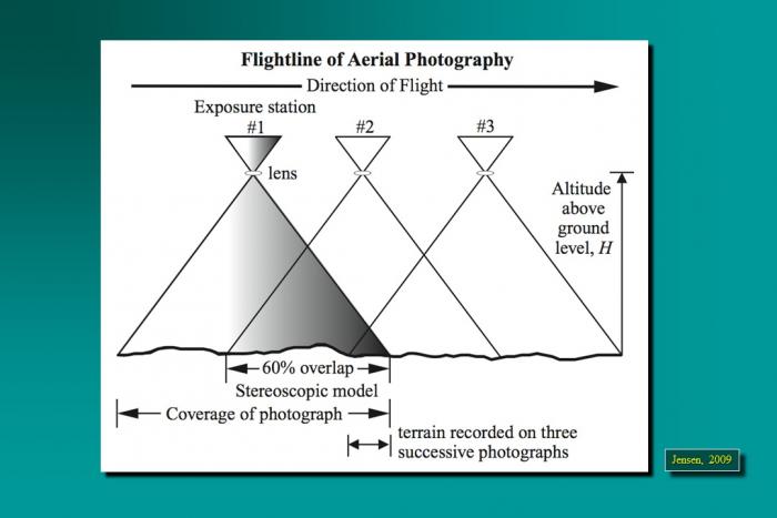
By extension, we could have a large block of aerial photographs, overlapping in the direction of flight as well as between adjacent flight lines, all oriented relatively to each other. This block, once constructed, represents all of the intersecting bundles of light rays from all of the overlapping photos. You can imagine that many of the points will be seen in a number of photographs. In fact, with 60% forward overlap, every point in a single flight line is seen 3 times. If the point falls in the 30% sidelap area between two flight lines, it will be seen 6 times; six rays will all intersect at one point. Actually, because some degree of measurement error is unavoidable, the intersection will occur within some sort of sphere, which represents the uncertainty in the projected coordinate of the point in question. As I mentioned earlier, the mathematical equations of photogrammetry allow us to quantify this uncertainty in statistical terms. Your readings will take you into greater depth and detail, but I hope my explanation helps you create a 3-dimensional picture in your mind, making the readings easier to understand.
Acquisition of Aerial Photography
For most photogrammetric mapping purposes, the goal is to image as much of the actual ground surface as possible. For this reason, it is customary to fly projects when deciduous trees are without leaves, when the ground is clear of snow and ice, when lakes and streams are within their normal banks, and when the sun is high overhead, minimizing shadows. In many parts of the world, this limits the optimal season for mapping to early spring, when days are getting long, but trees are relatively bare. Add the need for cloud-free skies to all these other requirements, and you can see why the flight operations of most photogrammetric mapping companies are not a big profit center. For any given location, there are a relatively small number of days per year when all the conditions are right for image acquisition.
By the way, these requirements are no different for space-based image acquisition. You already know that the orbits of passive imaging satellites are designed to follow local noon. That takes care of the time of day requirement. Add in all the other requirements, plus the constraints of orbital parameters and revisit times, and you can easily see why large-scale state and county mapping projects are still accomplished with aircraft. I'm sure we'll eventually see seamless coverage of states and nations with large-scale (1 meter/pixel GSD or better) satellite imagery, but it won't all be taken in the same season or even in the same year. Not until there are many, many more high-resolution imaging satellites circling the globe.
Sample Aerial Photography Specifications from Indiana Department of Transportation [2]
Aerial Imagery Guidelines from URISA Quick Study [3]
Several key computations related to flight planning are identified in these documents. These are:
- flight altitude above the ground required to achieve specified photo scale
- number of flightlines required to cover project area
- distance between (and total number of) flightlines required to achieve specified sidelap
- distance between (and total number of) successive exposures to achieve specified overlap
- total number of exposures required to complete project
In most aerial photography contracts, the aerial survey company provides a flight plan, based on customer specifications for scale and resolution, that enumerates all of the quantities outlined above along with a cost estimate based on those quantities.
Control and Georeferencing
The subject of control and georeferencing of a photogrammetric block could be the subject of several lessons in a course dedicated entirely to photogrammetry. I'm going to do my best to explain it conceptually without the math. Earlier in this lesson, you learned about the six parameters of exterior orientation that define the geometric relationship between an aerial photograph and the ground. I explained space resection and the way a minimum number of ground points can be used to solve the exterior orientation of a single vertical photograph. You may have thought to yourself how labor-intensive, expensive, and impractical it would be to actually solve the exterior orientation of each individual photograph in a large block by this method.
Photogrammetric mapping, based on very large blocks of hundreds or even thousands of aerial photographs, was made practical by the development of a technique called aerotriangulation, sometimes also called aerial triangulation, and often abbreviated as “A/T.” This short video from ASPRS [4] gives an overview of the concept, but a deep understanding comes from either years of training under a master, or a rigorous study of the mathematics. My reference to a master may sound a little overblown, but in my years of experience managing photogrammetric projects, a bad aerotriangulation solution that goes undetected is one of the most costly and time-consuming problems to correct. A/T is usually performed by the most experienced photogrammetrist in the organization, and there simply aren't that many true experts in it, perhaps a thousand or two at most worldwide. There are many software programs available to compute an A/T adjustment, but it’s easier to get a bad result than a good one, especially if the person designing the block and evaluating the statistical results doesn't have a deep theoretical understanding combined with a lot of practical experience.
The easiest way I have found to simply explain the concept of aerotriangulation is an extension of my desktop analogy. Picture again the bundles of intersecting rays generated by two overlapping photographs; the figure below depicts 3 photos in a single flight line. Now extend that picture in your mind's eye to include a second flight line "side-lapping" the first, also imaging points A, D, and G on the ground.
Point D, for example, is seen from 3 perspectives in the first flight line, and from another 3 perspectives in the side-lapping flight line I've asked you to visualize. Imagine that both flight lines continue on with many more end-lapping photos. All points common to adjacent flight lines, such as points D, G, and beyond, are going to be viewed with 6 intersecting rays. Even if we did not have a ground coordinate for every single one of these "tie points," you can imagine that, by enforcing the condition that the 6 rays must precisely intersect, there is still a lot of geometric stability in the block. This is the basic premise of aerotriangulation: enforcing the collinearity condition and the redundant intersection of image rays in "object space" creates a bridge from one photo to the next, thereby reducing the amount of ground control needed to reconstruct the exterior orientation for every photo.
If GPS/IMU direct georeferencing is available, the effect is to add additional control at each of the camera focal points, the photo centers, as they are often called. Remember that direct georeferencing gives us the 6 parameters of exterior orientation for every photo. We can use the direct georeferencing measurements as the first approximation of the aerotriangulation solution, and we no longer need actual ground control points. The GPS/IMU measurements for each photo center will inevitably contain errors, but we can reduce the impact of these errors in subsequent iterations of the block adjustment computation, simply by enforcing ray intersection for all the image tie points. This is done mathematically for all photos in the entire block simultaneously, and the A/T results give the photogrammetrist a quantitative assessment of the "goodness of fit" for this system of many redundant observations.
Photogrammetric Data Collection
Stereoplotters and Photogrammetric Workstations
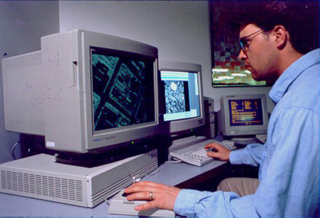
A stereoplotter is an instrument that can be used to recreate stereo models, so that a 3-dimensional model of the ground can be viewed, measured, and mapped by an operator. Compare the historical stereoplotters in the Lesson 1 reading to the softcopy workstation shown below. Binoculars have been replaced with other, less restrictive, forms of 3-dimensional viewing. In the example below, the glasses worn by the operator are polarized so that his right eye is seeing one image of the stereo pair, and his left eye is seeing the other.
Feature and Elevation Collection
Prior to the advent of digital workstations, map features were scribed by photogrammetric technicians on a drawing table integrated into the stereoplotter apparatus, often employing a pantograph [5] to enlarge the drawing to the final, desired map scale. Skilled cartographers would then use colored inks on semi-transparent materials, such as mylar, to create master map sheets that could be reproduced by blueprint or photo offset processes. These cartographers would add labeling and annotation as required. The final map was as much a work of art as it was a feat of technology. Today, feature data can be easily captured as 2-dimensional or 3-dimensional points, lines, and polygons when a Computer Aided Design (CAD) or GIS system is integrated into the softcopy workstation. Points might describe the location of fire hydrants, light poles, or simple building locations; lines could represent road or stream edges and centerlines; polygons are often used to represent detailed building footprints, stands of vegetation, water bodies, etc. In either a CAD or GIS package, each feature can be collected with unique line styles, line weights, and colors. If GIS software is used, the operator can also collect attribute information, such as road surface material, or building type, insofar as he can interpret this information from the aerial photograph.
Elevation data can be captured in a variety of ways; as in the case of feature data, methods have evolved along with photogrammetric technology. The earliest method for collecting elevation data was to manually draw isolines of elevation, or contours. It requires a great amount of skill and experience for an operator to draw spatially accurate, aesthetically pleasing contours. Contours are still one of the most effective representations of 3-dimensional topography on a 2-dimensional map; they are laborious to draw by hand, and while they can be generated automatically in a number of software packages, it usually requires a lot of manual editing to smooth jagged lines, to remove small artifacts, and to add labels. Many engineers learned to use contours early in their careers and still prefer them to other more modern, automated forms of digital elevation data.
Profiling is a technique of elevation data capture that was used extensively by the USGS and many private firms to create elevation data intended for input into the orthorectification of imagery. In this method, the stereoplotter is set to automatically drive the digitizing mark in evenly spaced profiles running the length or width of the stereo model. The operator's job is to keep reading elevations as accurately as possible in this dynamic environment; the stereo plotter automatically records elevations at regular intervals. The end result is a grid of regularly spaced points, which may or may not correspond to interesting or significant features of the actual terrain. This method of profiling works best in flat areas and in applications where accuracy and detail are not required. It was used quite a bit in the early days of orthophoto production, but is less common today.
Most elevation data derived from photogrammetry today is captured as randomly spaced mass points and breaklines. The photogrammetric technician collects individual 3-dimensional points at whatever frequency and in whatever pattern he deems appropriate to represent the ground surface. In addition, important linear features, such as road edges, curbs, walls, ridges, drains, etc., are captured as 3-dimensional lines. The mass points and breaklines are combined using surface modeling software to create a triangulated irregular network, or TIN. These elevation data products will be explained in more detail in the next lesson.
Image Data Products
Orthophotos
The term orthorectification refers to the process that removes effects of relief displacement, optical distortions from the sensor, and geometric perspective from a photograph or digital image. In a normal photograph, objects closer to the camera appear larger than objects of equal size that are further away from the camera. This presents an obvious difficulty in measuring objects accurately or determining their precise location in a reference coordinate system. In order to use perspective imagery as a map or in a geographic information system (GIS) environment, these geometric distortions must be corrected. The resulting image is referred to as an orthophoto or orthoimage.
Orthoimages can be created from any perspective image, regardless of the source, as long as three things are known:
- interior orientation, which describes the internal geometry of the camera system;
- exterior orientation, which describes the geometric relationship between the image and the ground;
- shape of the ground surface, which must be known in order to remove the effects of relief displacement. A digital terrain model must be supplied as input to the orthorectification process, in addition to the internal and external sensor geometry described above.
Returning to our familiar desktop example, the orthoimage is what would result if we took the 3-dimensional model created by all the intersecting light rays and projected every point straight down from the ground surface to an arbitrary flat plane. Each point would be in its appropriate planimetric (x, y) location, and all the effects of relief would be removed. The resulting image would have the exact same scale everywhere.
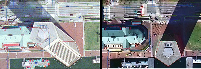
An orthophoto created using an elevation model representing only the bare ground surface will exhibit building lean everywhere except directly below the vantage point of the camera. All USGS and USDA orthophotos are created this way, as are the vast majority of state, county, and municipal orthophotos. On page 188 of Jensen (2007), he shows a comparison of this type of ground orthophoto to a true orthophoto, one which was created using a surface model comprising all of the above ground features at their proper elevation. True orthophotos are preferable in dense urban areas where the lean of tall buildings would obscure many important features on the ground between buildings. Building lean is also very distracting to GIS users, when they overlay building footprint data on top of an orthophoto backdrop. In a true orthophoto, the building footprints will line up with the images of the rooftops; in a ground orthophoto, they will not. Even though both datasets may be equally accurate and correct, the map still doesn't "look right."
Orthophoto Product Specifications
The specification for a digital orthophoto product deliverable must stipulate a ground coordinate system, pixel dimensions, spatial accuracy requirements, and the image file format. These specification elements are usually driven by the end user's application.
Many GIS systems today allow for reprojection of coordinate systems on-the-fly. However, when a raster image such as an orthophoto is projected from one coordinate system to another, it often requires resampling of the pixels, which can degrade the image quality and introduce artifacts. It is also computationally intensive, and can be quite time-consuming if the project includes a large number of high-resolution images. It is usually preferable to have the orthorectification process output orthoimagery in the coordinate system the end user intends to use for analysis. If there are multiple end users with diverse applications, which is often the case, a discussion and agreement on an output coordinate system should be part of the initial project design.
The size of the output pixel must be defined before running the orthorectification process. Knowing the output coordinate system before defining the pixel size is helpful; if one will be working in feet, it is preferable to have pixels defined as a round number interval, such as 1 foot, or 0.5 feet. Likewise for a metric coordinate system, pixel sizes of 1 meter, 50 cm, 30 cm or 25 cm are common. Finally, the GSD of the raw imagery should be considered; there is no point to creating an orthoimage with 25 cm pixels from an input image with a nominal GSD of 1 meter. It is customary to choose an output pixel size slightly larger than the nominal GSD of the input image; for example, if the output pixel size desired is 1 meter, then the project is usually designed for acquisition of data at a nominal GSD of slightly less than 1 meter, such as .8 or .9. This allows for the variation of actual GSD during acquisition due to perspective and relief, as described above, without compromising the spatial resolution of the end product.
Spatial accuracy of the end product depends on the quality of the georeferencing, either as inferred from ground control or provided by direct georeferencing technology. Spatial accuracy and pixel size (GSD) are completely unrelated. The size of a pixel has no physical bearing on the accuracy of its location in the ground coordinate system. However, in practice, it is customary when circumstances permit, to specify a spatial accuracy requirement that is comparable to the size of a pixel in ground units. For example, if the specified pixel size is 1 foot, then the spatial accuracy requirement might be defined such that each 1-foot pixel in the image was assured to be within 1 or 2 feet of its "true" location in the ground coordinate system. This is the ideal. In practice, depending on the end user application, it is not always possible or necessary to follow this rule. If the primary purpose of the imagery is simply to identify objects and measure their size relative to each other, then the absolute spatial accuracy in terms of ground coordinates may be less important. But generally, the rule of thumb is to target a root-mean-square-error (RMSE) for spatial accuracy equivalent to the size of a pixel in the output image. It should be noted, in case it is not already clear, that an orthoimage only has a spatial accuracy component in the horizontal. There is no elevation component to the orthoimage; it is strictly a 2-dimensional product, even though a 3-dimensional terrain model was required in order to produce it.
Image Data Formats
Image data are rasters, stored in a rectangular matrix of rows and columns. Radiometric resolution determines how many gradations of brightness can be stored for each cell (pixel) in the matrix; 8-bit resolution, where each pixel contains an integer value from 0 to 255, is most common. Modern sensors often collect data at higher resolution, and advanced image processing software can make use of these values for analysis. The human eye cannot detect very small differences in brightness, and most GIS software can only read an 8-bit value.
In a grayscale image, 0 = black and 255 = white; and there is just one 8-bit value for each pixel. However, in a natural color image, there is an 8-bit value for red, an 8-bit brightness value for green, and an 8-bit value for blue. Therefore, each pixel in a color image requires 3 separate values to be stored in the file. There are three possible ways to organize these values in a raster file.
- BIP - Band Interleaved by Pixel: The red value for the first pixel is written to the file, followed by the green value for that pixel, followed by the blue value for that pixel, and so on for all the pixels in the image.
- BIL - Band Interleaved by Line: All of the red values for the first row of pixels are written to the file, followed by all of the green values for that row followed by all the blue values for that row, and so on for every row of pixels in the image.
- BSQ - Band Sequential: All of the red values for the entire image are written to the file, followed by all of the green values for the entire image, followed by all the blue values for the entire image.
Orthoimages are delivered in a variety of image formats, compressed and uncompressed. The most common are TIF and JPG. Compression eases data management challenges, as large high-resolution orthophoto projects can easily result in terabytes of uncompressed imagery. Compression can also speed display in GIS systems. The downside is that compression can introduce artifacts and change pixel values, possibly hampering interpretation and analysis, particularly with respect to fine detail. The decision to compress should be driven by end user requirements; it is not uncommon to deliver a set of uncompressed imagery for archival and special applications along with a set of compressed imagery for easy use by large numbers of users. If there is an intention for web-based display or distribution of orthoimagery, a compressed set of orthoimagery is often recommended. In any event, georeferencing information must also be provided. Both TIF and JPG image formats can accommodate georeferencing information, either imbedded in the image file itself, as in the case of GeoTIF, or as a separate file for each image, as in the case of TIF with a TFW (TIF World) file. The georeferencing information tells GIS software 1) the size of a pixel, 2) where to place one corner of the image in the real world, and 3) whether the image is rotated with respect to the ground coordinate system.
Other popular image formats you may encounter are:
- ECW [6]: developed by ERMapper, now owned by ERDAS. Uses wavelet compression to reduce file size.
- GRID [7]: developed by Esri; supported by some remote sensing software packages, but not as common as other formats.
- IMG [8]: developed by ERDAS for Imagine; supported by many GIS and remote sensing software packages.
- JP2 [9]: JPEG 2000, developed by JPEG group. Widely supported by most GIS and remote sensing software packages.
- SID [10]: MrSid, developed by Lizard Tech. Uses wavelet compression to reduce file size. Read by many software packages, but requires proprietary software license to create.