Lesson 8: Terrain Modeling and Analysis
Lesson 8 Introduction
The elevation data products discussed in Lesson 4 provide representations of the three-dimensional landscape in several common GIS data structures: raster, point, and TIN surface. They may or may not include natural and man-made features (vegetation, buildings, bridges, etc.). In any application, the next step is usually to use one or more of those data structures to do some sort of analysis. In this lesson, we will examine several types of analyses that give us additional information about the terrain surface itself. The output from these analyses can be suitable for visualization of topography (contours and shaded relief maps), they can be an interim step in a more complex GIS analysis (slope and aspect maps), or they can predict the way the land and other physical elements of the landscape interact (flood inundation and optical line-of-sight). Since "topography" is defined as "the study of the Earth's surface shape and features,"1 the methods we will study in this lesson are often referred to as "topographic" analyses.
Lesson Objectives
At the end of this lesson, you will be able to:
- use both imagery and terrain data to create 3D visualization;
- perform a simple slope and aspect analysis;
- perform a simple hydrology analysis;
- perform a simple line-of-sight analysis.
Questions?
If you have any questions now or at any point during this week, please feel free to post them to the Lesson 8 Questions and Comments Discussion Forum in Canvas.
1Topography [1]. (2009, May 17). On Wikipedia, The free encyclopedia. Retrieved May 2, 2009
3D Visualization
Not very long ago, creating a 3D perspective view or a 3D fly-through of a scene in GIS was an arduous task. Today, it is nearly taken for granted that 3D views, animations, and analyses can be quickly and easily created and shared in posters, presentations, and with numerous web-based applications. Blending imagery and terrain in shaded relief is a standard feature of many interactive mapping tools, and these renderings are delivered to desktop and mobile platforms in the blink of an eye. However, the student of this course should, at this point, have an appreciation for both the data and computing infrastructures that are efficiently working behind the scenes. Without the availability of consistent, seamless, high-resolution imagery and elevation across nations and continents, there would be a limited market; the broad availability of high-quality data made available by publicly-funded programs at the federal and state level has made it worthwhile for private companies to invest in software and platform development. Recent leaps forward in data storage and dissemination capability make it feasible to serve these vast amounts of data to hundreds, even thousands, of simultaneous users.
Students who are taking this course are likely familiar with the concepts of 3D visualization from the end user's perspective. They may also be interested in learning to create effective 3D visualizations that blend imagery, terrain, and even detailed above-ground features for decision-making. The tools to create these visualizations are included in ArcGIS 3D Analyst, as well as in many other popular commercial GIS and CAD packages; they are not difficult to master. The quality of a visualization will depend largely on the informed selection of appropriate data using knowledge and skills presented in earlier lessons of this course.
Slope, Aspect, and Hillshade
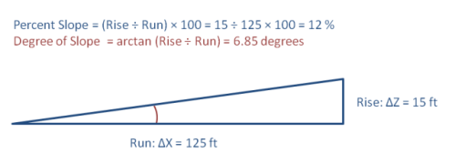
Slope is the steepness or the degree of incline of a surface. Slope cannot be computed from the lidar points directly; one must first create either a raster or TIN surface. Then, the slope for a particular location is computed as the maximum rate of change of elevation between that location and its surroundings. Slope can be expressed either in degrees or as a percentage. Aspect is the orientation of slope, measured clockwise in degrees from 0 to 360, where 0 is north-facing, 90 is east-facing, 180 is south-facing, and 270 is west-facing.
Hillshading is a technique used to visualize terrain as shaded relief, illuminating it with a hypothetical light source. The illumination value for each raster cell is determined by its orientation to the light source, which is based on slope and aspect. In the lab activity, you will experiment with placement of the light source, but, for now, it will suffice to say that positioning the light source in the northwest works best to simulate a natural landscape to the human eye. Depending on your application, you might also want to simulate the true position of the sun at a particular date and time of year.
Flood Inundation Analysis
True flood modeling, such as that used to produce FEMA's Digital Flood Insurance Rate Maps [3] (DFIRMs), is a complex process that includes terrain data, rainfall runoff or coastal storm surge models, hydrologic modeling, and hydraulic analysis. To determine the potential depth of flooding, one must be able to predict how much water is in the watershed at any given time, how that amount of water changes over time during a storm event, and how the flow of water is impeded or obstructed by vegetation or man-made structures. Floodplain mapping comprises an entire engineering discipline in its own right, and while GIS tools are extensively employed, simple topographic analysis alone does not create an accurate flood map.
That said, there may be legitimate applications for a more simple inundation analysis, such as you will perform in this lesson's lab activity. One real-world example of this was the inundation of New Orleans during Hurricane Katrina. Once the levees broke, and the water began to inundate low-lying areas of the Ninth Ward, the floodwaters were contained by the terrain features (natural and man-made) and simply rose until a steady-state condition was reached. In the end, the floodwaters were truly and accurately represented by a flat surface, and the depth of flooding could be simply determined by subtracting the land elevation at a given location from the elevation of this flat water surface. You will perform this simple type of flood inundation analysis on a land surface created from lidar point data. It will be up to you to evaluate how realistic the results are, and how they should or should not be used to predict real-world events.
Read More
You can read about modeling of the New Orleans flood in these articles:
- Gesch, Dean. Topography-based Analysis of Hurricane Katrina Inundation of New Orleans. [5] US Geological Survey.
- Griesmer et al., May 2006. Hurricane Katrina and Disaster Recovery Geospatial Process for Damage Assessment [6]. Proceedings of the 2006 American Water Resources Association Specialty Conference: GIS and Water Resources IV.
Line-of-Sight Analysis
Line-of-sight (LOS), also called "viewshed analysis," can be used to determine what can be seen from a particular location in the landscape. Conversely, the same analysis also determines from where within the surroundings that location can be seen. The first prerequisite for an LOS analysis is obviously a three-dimensional surface model of the landscape. For most applications, the most meaningful result would take vegetation, buildings, and other objects into account - those features that are purposely removed from bare-earth digital elevation models (DEMs). Above-ground features are generally included in Digital Surface Models (DSMs) created from lidar data.
LOS has many potential uses in community planning and zoning, airport operations management, event security, or battlefield cover and concealment, for example. Most students immediately think of cell phone tower placement as an application for LOS. While topography certainly has an impact on cell phone coverage, as in the case of flood inundation, modeling cell phone signal propagation [7] is in reality a much more complicated problem. An LOS analysis can be useful for planning cell-phone tower placement, but, to truly model cell phone coverage, more sophisticated models must be employed.